4903.pdf

(1)

Strategies for Differential Proteomic Analysis by Liquid Chromatography-Mass Spectrometry

Jordan Thomas Stobaugh

A dissertation submitted to the faculty of the University of North Carolina at Chapel Hill in partial fulfillment of the requirements for the degree of Doctor of Philosophy in the

Department of Chemistry.

Chapel Hill 2012

(2)

(3)

ABSTRACT

JORDAN THOMAS STOBAUGH: Strategies for Differential Proteomic Analysis by Liquid Chromatography-Mass Spectrometry

(Under the direction of James W. Jorgenson)

As the field of proteomics has evolved, the analytical techniques used in this field of

research has also evolved, transitioning from primarily gel-based techniques to separations

based on liquid chromatography. Enzymatic digestion is often a first step for comprehensive

analysis, known as bottom-up proteomics, but this comes at a cost of greatly increasing the

sample complexity. Analysis of intact proteins, or top-down proteomics, is not without

difficulties either as both the chromatography and mass spectrometry are more challenging.

Various single and multidimensional techniques have been used to increase the peak capacity

for bottom-up approaches, as, for the time being, they appear better suited for comprehensive

proteomic analyses.

The focus of Chapter 2 is determining what is possible given commercial

instrumentation and common analytical methods for a bottom-up analysis. A single- and

multidimensional separation were compared in the analysis of differentially grown yeast

samples. These same samples were used in Chapter 3 in a pre-fractionation approach in

which the intact protein samples were fractionated, then digested. The digested fractions

were then analyzed by LC/MS to determine protein identity and relative abundance. The

work presented in Chapter 5 relies on the methods developed in Chapter 3 in the differential

(4)

Lastly, in an effort to increase the number of protein identifications without

substantially increasing analysis time, new instrumentation was designed to facilitate

chromatography at pressures not attainable with commercial instrumentation. This was the

focus of Chapter 4 where a nanoAcquity UPLC was modified for XUPLC operation,

allowing for an increase in backpressure from 10,000 psi to 40,000 psi. With the increase in

back pressure, columns with more efficiency either through smaller particle diameters or

(5)

ACKNOWLEDGEMENTS

None of the work presented in this dissertation would have been possible without

contributions on many levels from many individuals. It would only seem appropriate to begin

with Dr. Jorgenson. Through his approach to research and guidance of students, I was able to

grow tremendously as a researcher with significant latitude to try new things, but lean on his

expertise for advice when needed. I cannot thank him enough for the opportunities provided

to me by studying under his direction. Brenna Richardson taught me many of the techniques

as a new graduate student that were needed for this research, and for that I am grateful. I also

must thank Kaitlin Fague, who worked alongside me for much of the work and will be

carrying the projects forward. Keith Fadgen and Martin Gilar from Waters Corporation

deserve many thanks as well. They each provided much support by aiding in troubleshooting

and for supplying the necessary parts to keep the systems operational. No data would have

been collected without their continued support. Keith has also been instrumental in providing

critiques for the XUPLC system. With regard to the motivation for the XUPLC system, Ed

Franklin was instrumental in showing what could be accomplished through use of long

capillary columns.

There are many people who helped me on a personal level during my time as a

graduate student. For helping me stay sane by providing me an outlet I need to thank the

students and mentors of FIRST Robotics Team 900, whom I mentored for three years. In

(6)

in mentoring and the fun we had while doing so. Nicholas Dobes also deserves a thank you

for the amusing opportunities he provided for me with car repair and other such tasks

involving my garage. Laura Blue also provided much support and stress relief through

conversations at our desks when everything seemed to be going wrong. Lastly, I must thank

my family for their unwavering support – my mother for helping to keep things in

perspective and my father for his guidance and valid opinions on my research. Megan, my

wife, probably deserves the most gratitude of all. Thank you for everything. Thank you for

moving far from home, leaving family, friends, and a career behind to allow me to pursue my

dreams. Thank you for Abigail, our daughter, and the joy she has brought us. None of this

(7)

TABLE OF CONTENTS

LIST OF TABLES ... xii

LIST OF FIGURES ... xiv

LIST OF ABBREVIATIONS ... xxviii

CHAPTER 1: INTRODUCTION AND BACKGROUND FOR PROTEOMICS BY MULTIDIMENSIONAL LIQUID CHROMATOGRAPHY MASS SPECTROMETRY ...1

1.1 Differential Proteomics ...1

1.1.1 Definition and Challenges ...1

1.1.2 Approaches: Top-Down vs. Bottom-Up ...2

1.1.4 Quantitative proteomics ...4

1.2. Multidimensional separations for differential proteomics ...7

1.2.1 Background and theory ...7

1.2.2 Two-dimensional gel electrophoresis ...10

1.2.3 Gel-Eluted Liquid-Fraction Entrapment Electrophoresis ...11

1.2.4 Multidimensional peptide identification technology ...12

1.2.5 Pre-fractionation as alternative MDLC approach ...13

1.3 Scope of Dissertation ...15

1.4 References ...16

(8)

2.1 Introduction ...21

2.1.1 Bottom-up Proteomics ...21

2.1.3 Ion mobility in proteomic applications ...24

2.2 Experimental ...25

2.2.1 Overview of experimental methods ...25

2.2.2 Preparation of S. cerevisiae protein extracts ...25

2.2.3 Trypsin digestion of fractions ...26

2.2.5 Capillary UPLC-MS/MS of tryptic peptides ...27

2.2.6 Protein identification by PLGS 2.5 & Scaffold 3.3. ...28

2.3 Results & Discussion ...28

2.3.1 Differential comparison of Baker’s yeast by 1D UPLC. ...28

2.3.2 Analysis of gradient length and available peak capacity. ...33

2.3.3 2D nanoAcquity ...35

2.3.4 Data from Synapt G2 ...38

2.4 Summary and Conclusions ...40

2.6 Tables ...44

2.7 Figures...45

CHAPTER 3: PRE-FRACTIONATION OF DIFFERENTIALLY GROWN S. CEREVISIAE CELL LYSATES ...62

3.2. Experimental ...63

3.2.1 Overview of Experimental Methods ...63

3.2.2 Chemicals and sample preparation ...64

(9)

3.2.5 Multidimensional LC/MS of peptides ...66

3.2.6 Peptide data processing ...67

3.3.1 Chromatograms of Intact Protein Separations ...68

3.3.2 Proteins per fraction ...71

3.3.4 Fractions per protein ...76

3.3.5 Molecular weight distribution of identified proteins ...77

3.3.6 Differential comparison for RP-20 & AXC-20 fractionation strategies ...78

3.4 Conclusions ...82

3.6 Tables ...87

3.7 Figures...89

CHAPTER 4: XUPLC MODIFICATION OF A NANOACQUITY UPLC ...109

4.1.1 Motivation for ultra-high pressure separations ...109

4.1.2 Previous prototype instrumentation ...111

4.1.3 Purpose of nanoAcquity modification ...113

4.2 System design & experimental parameters ...114

4.2.1 Pneumatics ...114

4.2.2 Fluidic connections ...116

4.2.3 Flow paths ...118

4.2.4 Software interface ...119

4.2.5 Constant Pressure & Elevated Temperature ...122

4.2.6 Columns & Running conditions ...124

(10)

4.3.1 Gradient Clipping...125

4.3.2 Leaks ...125

4.3.3 Data Analysis of linked files ...126

4.3.4 Chromatographic performance of XUPLC ...127

4.4 Future directions ...132

4.6 Tables ...136

4.7 Figures...137

CHAPTER 5: APPLICATION OF PRE-FRACTIONATION METHODOLOGY FOR A DIFFERENTIAL ANALYSIS OF A MOUSE EMBRYONIC FIBROBLAST BETA-ARRESTIN 1,2 DOUBLE-KNOCKOUT ...166

5.1.1 Beta-arrestin background ...166

5.1.2 Previous studies of MEF lysates by online 2DLC ...169

5.2 Experimental ...169

5.2.1 Overview of experimental method ...169

5.2.2 Preparation of MEF protein extracts ...170

5.2.3 LC/MS conditions ...171

5.3.1 Comparison of AXC40 to RP18 ...172

5.3.2 Comparison of Pre-fractionation to Online 2DLC results ...177

5.3.3 Comparison of Pre-fractionation to Literature ...179

5.3.4 Comparison of MEF to Yeast ...182

5.4 Conclusions ...183

(11)

5.5.2 XUPLC of peptides ...185

5.5.3 Immunoprecipitation of beta-arrestin interacting proteins ...185

5.6 Tables ...187

5.7 Figures...190

(12)

LIST OF TABLES

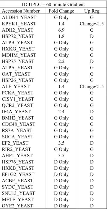
Table 2-1. Proteins identified as being differentially expressed between the dextrose-based and glycerol-dextrose-based baker’s yeast samples are shown here. These proteins were found to have a P-value of less than 0.05 when conducting a Fisher’s exact

test. ...44

Table 3-1: Gradient program used for the intact protein pre-fractionation of the yeast cell lysates by anion-exchange chromatography. The column used was a Waters BioSuite Q SAX, 7.5 mm ID x 7.5 cm with 10 μm particles and 1000 Å pores. The flow rate was 0.5 mL/min and the column was held at a temperature of 50 °C, the maximum per manufacturer recommendations. Forty fractions were

collected from 2 to 82 minutes. ...87

Table 3-2: Gradient program used for the intact protein pre-fractionation of the yeast cell lysates by reversed-phase chromatography. An Agilent PLRP-S, 4.6 mm x 25 cm column with 5 μm pores particles and 300 Å pores. The flow rate was 1.0 mL/min. A column temperature of 80 °C was used – well below the rated maximum of 200 °C. Fractions were collected every minute from 2 to 42

minutes for a total of 40 fractions collected. These fractions were later pooled to

form the 20 fractions analyzed. ...87

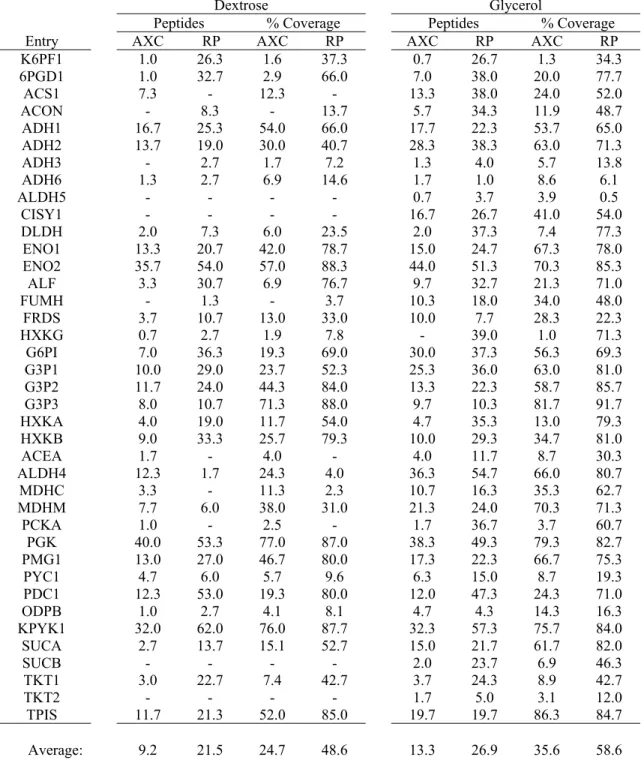
Table 3-3: The number of peptides used in an identification as well as the coverage percentage of the proteome is shown for both anion-exchange and reversed-phase pre-fractionation of proteins determined to be involved in the metabolic pathways of interest and differentially expressed. Overall, there were more peptides found

and a larger coverage percentage for the reversed-phase pre-fractionation. ...88

Table 4-1. Three columns were evaluated on the XUPLC system. These include a 200-cm column packed with 1.9 μm particles, a 117-cm column packed with 1.5 μm particles, and a 25-cm column packed with 1 μm particles. The inner diameter for each column was 75 μm. The pressure supplied by the Haskel -903 pump was approximately 30,000 psi and the temperature was held at 65°C. Gradients of water and acetonitrile were used to elute the peptides and started between 1% & 3% acetonitrile with a final acetonitrile concentration of 40% at the end of the gradient. Peak capacities were calculated by dividing the elution window, which was defined as the period of time between the first eluting peak and last eluting peak, by the FWHM peak width. The analysis time corresponds to the amount of time required from injection-to-injection. Detection was by a Waters QTOF Premier mass spectromter. Proteins were identified with PLGS 2.5. The last two lines of the table show data from a standard nanoAcquity setup utilizing a 90-minute gradient previously determined as the preferred gradient length with one data set collected with a QTOF Premier and the other with a Waters Synapt G2

(13)

Table 5-1. Gradient program used for the intact protein pre-fractionation of the yeast cell lysates by anion-exchange chromatography. The column used was a Waters BioSuite Q SAX, 7.5 mm ID x 7.5 cm with 10 μm particles and 1000 Å pores. The flow rate was 0.5 mL/min and the column was held at a temperature of 50 °C, the maximum per manufacturer recommendations. Forty fractions were

collected from 2 to 82 minutes. ...188

Table 5-2. Gradient program used for the intact protein pre-fractionation of the yeast cell lysates by reversed-phase chromatography. An Agilent PLRP-S, 4.6 mm x 25 cm column with 5 μm pores particles and 300 Å pores. The flow rate was 1.0 mL/min. A column temperature of 80 °C was used – well below the rated maximum of 200 °C. Fractions were collected every minute from 2 to 42

minutes for a total of 40 fractions collected. These fractions were later pooled to

form the 20 fractions analyzed. ...188

Table 5-3. Proteins found by the anion-exchange pre-fractionation method that are known to associate with beta-arrestin proteins are shown here. Only 5 of the 18 proteins in this list were differentially expressed and found in both samples allowing a fold change to be calculated. Nearly half, 7 of 18, were found to be

expressed within a fold change of 1.5 in each sample. ...189

Table 5-4. For the reversed-phase pre-fractionation, there were fewer proteins

identified that are known to interact with the beta-arrestin proteins. There were a few differences between this data and that from the anion-exchange

pre-fractionation data as fold changes were calculated for some of the tubulin

(14)

LIST OF FIGURES

Figure 2-1. a) During the first dimension of separation, flow from the first pump at a pH of 10 flows through the first-dimension column. Effluent from this column is diluted with low pH mobile phase from the second pump before being trapped on the trap column. During the second dimension of analysis (b), flow from the first pump is diverted after the first-dimension column to waste and a gradient is pumped from the second pump through the analytical column with detection by

mass spectrometry. ...45

Figure 2-2. The separation of peptides from the dextrose-based sample and glycerol-based sample was by reversed-phase UPLC with a 60 minute long gradient from 5-40% acetonitrile. For the purposes of a differential comparison, proteins were only counted if they were identified with a confidence greater than 95% by Scaffold 3.3 in two of three replicates. This figure indicates the number of proteins identified in each sample and the number of proteins identified in common. For the differential comparison, proteins were required to have a

p-value less than 0.05 after a Fisher’s exact test was applied to the data. ...46

Figure 2-3. Given the change in carbon source from dextrose to glycerol, it was expected that there would be differences in protein expression for the metabolic pathways. Simplified pathways and their associated proteins are shown here. Proteins found to be regulated in glycerol are shown in red. Those up-regulated in the dextrose sample are shown in blue. Proteins identified, but not determined to be differentially expressed are shown in boldface black with unidentified proteins shown in gray. The gradient length used in the peptide

separation was 60 minutes in length from 5-40% acetonitrile. ...47

Figure 2-4. Additional gradient lengths were attempted. The gradient lengths used were (a) 90-, (b) 120-, (c) 150-, and (d) 180-minutes. For the purposes of a differential comparison, proteins were only counted if they were identified with a confidence greater than 95% by Scaffold 3.3 in two of three replicates. This figure indicates the number of proteins identified in each sample and the number of proteins identified in common. For the differential comparison, proteins were required to have a p-value less than 0.05 after a Fisher’s exact test was applied to

the data. ...48

(15)

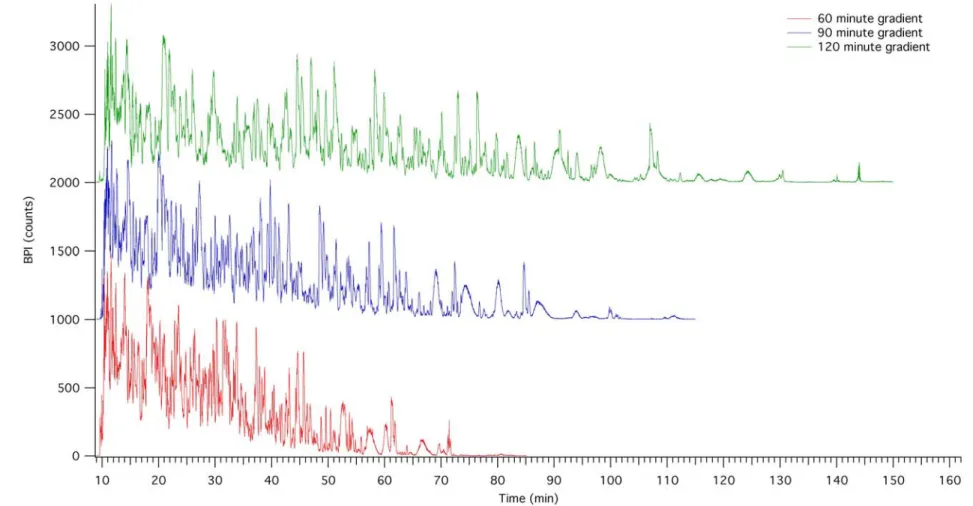
Figure 2-9. Representative chromatograms of the glycerol-based, yeast cell lysate digest for gradient lengths of , 90-, and 120-minute long gradients. The 60-minute method shows a chromatogram that is crowded with poorly resolved peaks. This improves slightly with the 90-minute gradient. A more thorough analysis is needed than what is possible through visual inspection to determine

improvements to peak capacity. ...53

Figure 2-10 Representative chromatograms of the glycerol-based, yeast cell lysate digest for gradient lengths of 150- and 180-minute long gradients. For both of these gradients, it does not appear as though the resolution is improving. Peak widths are broader at the longer gradient times. A more thorough analysis is needed than what is possible through visual inspection to determine

(16)

Figure 2-11. From the chromatograms shown above, the data shown here is the result of the PLGS 2.5 data processing. The Apex3D algorithm used to process the raw mass spectral data attempts to fit Gaussian peaks to the eluting peptides. From this data, the full-width, half-maximum (FWHM) of the peaks are readily

available. Peak capacities here are calculated from the FWHM. Gradients longer than 90 minutes were not shown to give more protein identifications. There was a slight increase in peak capacity in lengthening the gradient from 90- to 120-minutes. At 180 minutes, the gradient becomes shallow enough and the peaks tail significantly enough that the Apex3D algorithm begins fitting multiple peaks

per actual peak. ...55

Figure 2-12. Proteins that were identified in one of three analyses with a confidence greater than 95% by Scaffold 3.3 are counted here. The multidimensional UPLC system utilizing a high pH first dimension and a low pH second dimension resulted in a greater number of identifications. The amount of time required for the multidimensional approach, however, was significantly more than required

of the single-dimension analyses. ...56

Figure 2-13. For the multidimensional peptide separation, the coverage of the metabolic pathways of interest was about the same as for the longer, single-dimension separations. The coverage was found to be 26 of the 53 proteins

searched for. ...57

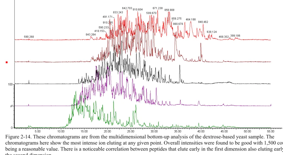
Figure 2-14. These chromatograms are from the multidimensional bottom-up analysis of the dextrose-based yeast sample. The chromatograms here show the most intense ion eluting at any given point. Overall intensities were found to be good with 1,500 counts being a reasonable value. There is a noticeable correlation between peptides that elute early in the first dimension also eluting early in the

second dimension. ...58

Figure 2-15. The chromatograms here are from the same analysis as in Figure 14. Here, the total ion current has been plotted, providing a clearer picture of the elution window and the correlation of peptides eluting early in the first

dimension also eluting early in the second dimension, as shown in green in the bottom trace. The percentage acetonitrile used to elute peptides from the first

dimension are shown for each fraction. ...59

Figure 2-16. All of the other metabolic pathway figures were comprised of data collected on a Waters QTOF Premier mass spectrometer. For this analysis, the same conditions used for the 90-minute gradient conducted in the Jorgenson lab were used by the Duke Proteomics Core facility to obtain data on their Waters SynaptG2 HDMS mass spectrometer. The newer and more advanced mass spectrometer, which also utilized an ion mobility separation, was able to identify

(17)

Figure 2-17. Scaffold 3.3 attempts to assign all peptides. Using the peptides score as part of this function, the software attempts to eliminate incorrectly assigned peptides from being used to identify proteins. Data was collected on two different mass spectrometers, (a) a SynaptG2 and a (b) QTOF Premier. There were a greater number of correctly assigned peptides from the SynaptG2 data and the differences in scores between the incorrect and correct populations were also greater. The improved data facilitated the additional identifications observed with the analysis completed by the more advanced mass spectrometer. ...61

Figure 3-1. Experimental workflow for the intact protein pre-fractionation and

bottom-up analysis of each digested fraction. An LC pump generated a gradient, which began the specified gradient program once the injection occurred. A Waters 2487 UV detector at 280 nm recorded data for the intact protein

separations. Fractions were then lyophilized and digested with trypsin. Fractions were then analyzed by either 1D or 2D-UPLC/MSE using a Waters nanoAcquity UPLC system with mass spectrometric detection by a Waters Q-TOF Premier mass spectrometer. The data was then processed through ProteinLynx Global

Server 2.5 and Scaffold 3.3. ...89

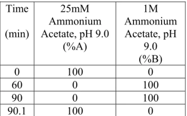
Figure 3-2. Anion-exchange pre-fractionation of yeast cell lysates differentially grown on dextrose and glycerol-based media. Approximately 4 mg of each sample was inject for analysis. The column used was a Waters BioSuite Q SAX, 7.5 mm ID x 7.5 cm with 10 μm particles and 1000 Å pores. The flow rate was 0.5 mL/min and the column was held at a temperature of 50 °C, the maximum per manufacturer recommendations. A linear gradient from 25 mm ammonium bicarbonate, pH 9.0 to 750 mM ammonium bicarbonate, pH 9.0, was run from 0-60 minutes with an additional 30 minute hold at 750 mM ammonium

bicarbonate. Forty fractions were collected from 2 to 82 minutes. For the

anion-exchange pre-fractionation, the intact protein separation was only done once. ...90

Figure 3-3. The initial separation of the dextrose yeast cell lysate on the PLRP-S column, an Agilent PLRP-S, 4.6 mm x 25 cm column with 5 μm particles and 300 Å pores. Mobile phase A was comprised of 80% water, 10% acetonitrile and 10% isopropanol plus 0.2% TFA. Mobile phase A was a 50/50 mixture of

acetonitrile and isopropanol with 0.2% TFA added. The temperature was held at 90 °C. This gradient was substantially steeper than the final gradient conditions used for the pre-fractionation, but demonstrated the utility of this column and

(18)

Figure 3-4. For the reversed-phase pre-fractionation methods, a more rigorous replicate analysis was employed to better evaluate the reproducibility of the entire method. As such, each intact protein sample injected three times with fractions collected and digested for each of the 6 runs. An Agilent PLRP-S, 4.6 mm x 25 cm column with 5 μm pores particles and 300 Å pores was used for the separations. The flow rate was 1.0 mL/min. A column temperature of 80 °C was used – well below the rated maximum of 200 °C. Fractions were collected every minute from 2 to 42 minutes for a total of 40 fractions collected. These fractions were later pooled to form the 20 fractions analyzed. For each sample, the UV traces overlay quite well demonstrating good method reproducibility. The

gradient conditions are overlayed in black and correspond to the right axis. ...92

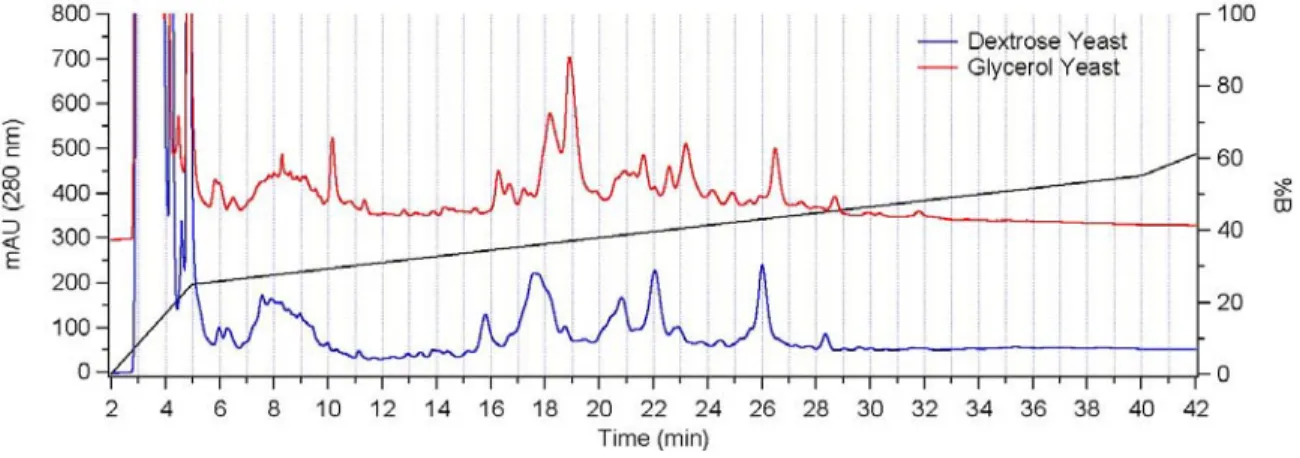
Figure 3-5. While the samples are very similar and show similar elution trends, there are also differences prevalent between the two sample types. The glycerol yeast data, offset by 300 mAU, show an intense peak at 10 minutes which is missing altogether in the dextrose yeast, as an example. The gradient conditions are

overlayed in black and correspond to the right axis. ...93

Figure 3-6. The total number of protein identifications for each fraction are shown in light grey. Plotting the data in this way is useful as it gives an idea as to what is eluting off of the LC column in each fraction and the complexity of the sample reaching the mass spectrometer. However, for the purpose of determining overall protein identifications, it is more convenient to represent the data by only

plotting proteins in the fraction of greatest intensity, as determined through Scaffold 3.3. Fewer identifications were made by the anion-exchange method (a) than by the reversed-phase method (b). For both intact protein separations, few

new unique proteins were identified in the final five fractions. ...94

Figure 3-7. The reversed-phase pre-fractionation method identified 546 proteins in 2/3 replicate runs whereas there were only 262 proteins identified in 2/3 replicate runs of the peptide fractions. Only 16% of the proteins identified by anion

exchange were not identified by the reversed-phase approach. Twenty fractions were analyzed by each method to allow for a uniform comparison based on

gradient fractionation. ...95

Figure 3-8. After running all 40 fractions from the anion-exchange pre-fractionation method, similar trends are observed as seen previously in Figure 6. The total number of protein identifications for each fraction are shown in dark red. Plotting the data in this way is useful as it gives an idea as to what is eluting off of the LC column in each fraction and the complexity of the sample reaching the mass spectrometer. However, for the purpose of determining overall protein identifications, it is more convenient to represent the data by only plotting proteins in the fraction of greatest intensity, as determined through Scaffold 3.3, and is shown in light red. Finer fractionation where there are large numbers of proteins eluting and courser fractionation over portions of the method where

(19)

Figure 3-9. For the anion-exchange approach, all 40 fractions were analyzed in addition to being pooled to form 20 fractions. Finer fractionation allowed for a small increase in the number of proteins identified, but required an increase in

analysis time from 120 to 240 hours. ...97

Figure 3-10. Reversed-phase pre-fractionation allowed for a greater number of protein identifications than either anion-exchange method. A total of 658 unique proteins were identified in at least 2/3 replicate runs for these fractionation

strategies. Only 17% (112) were not found by reversed-phase pre-fractionation. ...98

Figure 3-11. An alternative approach to increasing the fractionation of the intact protein separation was to increase the peak capacity of the peptide separation by incorporating a multidimensional separation at the peptide level. This

comparison was made by analyzing only the glycerol yeast sample. While a greater number of protein identifications were made with the multidimensional separation, it is questionable whether the gains in additional identifications are

worth the additional analysis time. ...99

Figure 3-12. A representative set of chromatograms from the reversed-phase

fractionation of yeast grown on glycerol. Reversed-phase chromatography was used in both dimensions of the peptide separation by operating the first

dimension at a pH 10 and the second dimension at pH 3. The first-dimension column was a custom-packed 150 μm ID x 10 cm XBridge C18 with 3.5μ particles and 130 Å pores. The second-dimension column was a Waters Acquity BEH C18 column with 1.7 μm particles and 130 Å pores. Five fractions were taken from the first dimension and peptides were eluted from the first column in five isocratic steps of 12, 16, 20, 24, and 65% acetonitrile. There is a general trend of peptides eluting early in the first-dimension also eluting early in the second-dimension suggesting a lack some level of correlation between the two

dimensions and limiting the peak capacity of the overall system. ...100

Figure 3-13. The percentage of unique proteins is plotted as a function of the number of fractions a unique protein is identified in. Both anion-exchange and reversed-phase pre-fractionation strategies exhibit similar behavior when compared on the basis of gradient fractionation. The majority of proteins (60%) elute in only one fractions indicating that the fractions were approximately equal to the width of a

peak. ...101

Figure 3-14. Only a slight increase in the number of fractions a unique protein was identified in was associated with the more comprehensive peptide analysis. It has been reported that greater peak capacity afforded by the multidimensional

separation allows for the detection of peptides at lower concentrations and

(20)

Figure 3-15. There was no bias associated with the molecular weight of the intact proteins identified by either pre-fractionation method. The median mass of proteins identified was 37.6 kDa for anion exchange (a) and 38.0 kDa for

reversed phase (b). ...103

Figure 3-16. The mass of proteins for the reversed-phase (a) and anion-exchange (b) pre-fractionation methods are shown as a function of the fraction each protein eluted in greatest intensity. More abundant proteins are represented by darker

bars. ...104

Figure 3-17. The reversed-phase pre-fractionation approach showed better overlap between the two samples than either anion exchange fractionation approach and significantly more proteins overall. While the samples were grown on different

carbon sources, a significant amount of agreement is expected between the two. ...105

Figure 3-18. Greater variability in the identified proteins was observed between the two samples when pre-fractionated by anion-exchange chromatography. In general, proteins identified by the anion exchange methods were less intense than by the reversed phase method suggesting that the decreased overlap

between the two samples may be due in part to poor recovery. ...106

Figure 3-19. By increasing the fractionation of the anion exchange method from 20 to 40 fractions, not only was there an increase in the number of identifications, but

better agreement between the samples with respect to the proteins identified. ...107

Figure 3-20. The up-regulation of the TCA cycle and the glyoxylate cycle are much more evident from the reversed-phase pre-fractionation approach. Many more proteins were identified by the reversed-phase method and these additional identifications were needed in order to form conclusions. The up-regulation of proteins in these pathways meets expectations given the nature of the differential

sample. ...108

Figure 4-1. The Apex3D algorithm used to process the raw mass spectral data attempts to fit Gaussian peaks to the eluting peptides. From this data, the full-width, half-maximum (FWHM) of the peaks are readily available. Peak capacities here are calculated from the FWHM. Gradients longer than 90 minutes were not shown to give more protein identifications. There was a slight increase in peak capacity in lengthening the gradient from 90- to 120-minutes. At 180 minutes, the gradient becomes shallow enough and the peaks tail

significantly enough that the Apex3D algorithm begins fitting multiple peaks per

(21)

Figure 4-2. The prototype hydraulic amplifier system previously used for automated UHPLC gradient analyses. During sample loading and gradient formation (A), flow would originate from the CapLC system and fill the gradient storage loop. After loading, the two “pin valves” or Valco on/off valves would be closed and the hydraulic amplifier activated, forcing flow out of the storage loop and

through the column and splitter. ...138

Figure 4-3. A Waters nanoAcquity UPLC with detection by a Waters QTOF-Premier

mass spectrometer. The pressure limit of the nanoAcquity is 10,000 psi. ...139

Figure 4-4. The nanoAcquity UPLC with the XUPLC modification installed.

Pneumatic components are primarily locatd on the left side of the nanoAcquity stack with the exception of the Valco on/off valves. The column heater is mounted to position the outlet of the capillary column near the mass spectrometer source. A gradient storage loop is wound around a spool and mounted below the temperature control module on the lower right of the

nanoAcquity. ...140

Figure 4-5. A general schematic for the pneumatics sub-system. Gas supply (air or N2) needs to be provided at approximately 100 psi. Two regulators are need, one to regulate down the pressure to 40 psi for the solenoid valves responsible for switching the Valco on/off valves and the other to supply pressure to the Haskel -903 pneumatic amplifying liquid pump. The outlet pressure of the -903 is

roughly equal to 1,000 psi liquid for 1 psi gas. ...141

Figure 4-6. A photograph of the pneumatics sub-system showing mounting locations. Note the ball valves for manual shut-off and release of gas pressure to the -903. These are installed as a safety mechanism in case rapid decompression is

required without the use of the computer controls. ...142

Figure 4-7. Fluidic schematic overview for the XUPLC system. The blue circles represent Valco on/off valves. Grey circles represent tees from Valco. The trap column, analytical column, and associated tees are housed inside the Waters

TCMII for elevated temperature operation. ...143

Figure 4-8. During gradient loading, the nanoAcquity vent valve and trap valve are closed. Flow from the nanoAcquity fills the gradient storage loop. The resistance to flow from the analytical column is sufficient enough to prevent the gradient

from being split between the storage loop and the column. ...144

Figure 4-9. During sample loading and trapping the valves are configured to allow flow from the nanoAcquity through the trap column and then to waste. Analytes are trapped on the column. Trapping conditions are typically 0.5% acetonitrile and a minimum volume of three times the sample loop volume is used to ensure all of the sample has been flushed onto the column. During this operation, the

(22)

Figure 4-10. During running operation the vent, nanoAcquity and trap valves are closed and the gradient storage isolation valve is opened. This forces flow driven by the -903 pump through the storage loop, past the trap column where analytes are eluted, and onto the analytical column where analytes are briefly re-focused prior to elution. The nanoAcquity vent valve is open during operation to prevent

damage to the nanoAcquity should the nanoAcquity valve fail. ...146

Figure 4-11. Typically, one line of the sample list corresponds to an LC/MS analysis. For XUPLC operation, a minimum of two lines and frequently more are required for a given sample injection. The first row is responsible for loading the gradient. The second line allows for the sample injection and starts the mass spectrometer. Often a third row is used to stop the analysis and return the system to initial conditions for the next run, although two can be used for shorter analyses. If more lines are needed, they can be added in an intermediate position in order to

maintain valve states for running operation. ...147

Figure 4-12. On the rear of the nanoAcquity are several switches required for XUPLC operation. These control the Valco on/off valves responsible for manipulating the flow path. In order to access these during manual operation, one must navigate to the “Rear panel…” menu under “Troubleshoot” for both the pump

and autosampler. ...148

Figure 4-13. Within the rear panel are many switches. The ones needed for operation are switches 1, 2, and 3 on the binary solvent manager rear panel and switches 1,

2, 3, and 4 on the sample manager rear panel. ...149

Figure 4-14. For automated operation, timing events are included in inlet file, which is the method file used by the nanoAcquity during operation. For both the pump and autosampler, there is an events tab where switches and their associated on/off states can be defined. To aid in method development, a spreadsheet was

developed to allow the user to more easily program the methods. ...150

Figure 4-15. Curves showing the change in viscosity as a function of the acetonitrile percentage and the temperature are shown here at 25, 45, 65, and 85°C spanning

0% to 100% acetonitrile. Most gradients range from 1-40% acetonitrile.13,14 ...151 Figure 4-16. Data shown in Figure 15 was normalized in order to demonstrate the %

change in viscosity. The figure was also modified to show the difference in

(23)

Figure 4-17. Method development for the XUPLC system is more difficult than for standard nanoAcquity UPLC operation. Clipping of the front-end of the gradient can occur if an incorrect delay time is used. The delay is necessary to account for the system volume between the pump and the gradient storage loop. This can be observed in the chromatogram shown as at 18.5 minutes there is a sudden change from baseline conditions to full-intensity peptide elution. A more appropriate delay volume would result in a gradual rise from the baseline as

peptides begin to elute. ...153

Figure 4-18. As a result of the elevated pressures (30,000 psi), leaks can develop. These are routinely found on the fused-silica capillary fittings. The volume of gradient loaded should have resulted in a nearly 300-minute long analysis time. From this chromatogram, it would appear as though a leak developed at

approximately 63 minutes. A leak is suspected as the gradient is unexpectedly progressing much more rapidly with a significant number of peaks being detected in a compressed timescale. The location of the leak is likely one of the three connections on the tee prior to the trapping column as there are still peptides being detected. A leak at the second tee results in a significant loss of

sample and no peaks are seen as a result. ...154

Figure 4-19. A 200-cm x 75 μm ID capillary column packed with 1.9 μm BEH C18 particles was operated at 30,000 psi and 65°C. The gradient was 35 μL of 4-40% acetonitrile. A peak capacity from the full-width, half-maximum data outputted from ProteinLynx yields a peak capacity of 660 for this separation. A total of

153 proteins were identified from this separation. ...155

Figure 4-20. A 117-cm x 75 μm ID capillary column packed with 1.5 μm BEH C18 particles was operated at 30,000 psi and 65°C. The gradient was 45 μL of 3-40% acetonitrile. A peak capacity from the full-width, half-maximum data outputted from ProteinLynx yields a peak capacity of 570 for this separation. A total of

128 proteins were identified in this separation. ...156

Figure 4-21. The elevated pressure permits the use of longer columns with modestly sized particles (1.5 and 1.9 μm). Also possible is the use of 1 μm particles. A 25 cm x 75 μm ID capillary column was packed with 1 μm BEH C18 particles and operated at 65°C. The gradient had a volume of 35 μL spanning 1-40%

acetonitrile. Run times more consistent with what is typically of the nanoAcquity UPLC are possible with this shorter column. In this analysis, 119 proteins were identified in a total analysis time of 120 minutes with a peak capacity of 250. For standard nanoAcquity operation, a 90-minute gradient resulting in a total run time of 120 minutes resulted in 80 protein identifications and a peak capacity of

(24)

Figure 4-22. A 25 cm x 75 μm ID capillary column was packed with 1 μm BEH C18 particles and operated at 65°C. The gradient had a volume of 25 μL spanning 1-40% acetonitrile. Run times more consistent with what is typically of the nanoAcquity UPLC are possible with this shorter column. In this analysis, 85 proteins were identified in a total analysis time of 120 minutes with a peak capacity of 250. The same peak capacity was the result of narrower peaks with this length of gradient as compared to the gradient used in for the chromatogram in Figure 22. The reduction in identified peaks can likely be attributed to the narrow peaks not being characterized as well by the Apex3D algorithm within

ProteinLynx...158

Figure 4-23. A 25 cm x 75 μm ID capillary column was packed with 1 μm BEH C18 particles and operated at 65°C. The gradient had a volume of 15 μL spanning 1-40% acetonitrile. In this analysis, 59 proteins were identified in a total analysis time of 120 minutes with a peak capacity of 160. This method requires 60 minutes from injection-to-injection and has a comparable peak capacity to the

nanoAcquity in 2/3 the analysis time. ...159

Figure 4-24. The same 117-cm column with 1.5 μm particles as used in the analysis shown in Figure 20 was used here with a gradient approximately twice the length. There was only a slight improvement in peak capacity and fewer proteins were identified. Close examination of the peak shape reveals substantial tailing. Mass overload is not suspected as this is exhibited by low intensity peaks as well. Reducing the mass of sample injected did not result in peak shape improvements either. The forward-trapping, forward-flush operation is suspected to be

contributing to this problem. The trap column is much longer (6.5 cm) than what is typically used in this type of operation on the nanoAcquity (2 cm). This additional length may be broadening the peaks sufficiently such that they cannot

properly focus at the head of the analytical column. ...160

Figure 4-25. Inside the column heater module are the trap column, analytical, and hardware required for operation. The two tees and either end of the trap column are mounted to a slotted piece of ¼” aluminum plate to facilitate assembly. The tees can be mounted with a screw from the back. The analytical column is coiled and taped to the surface of the heater to ensure that it is at the proper temperature. A Teflon junction is used to connect the outlet of the column, which remains inside the heater, to a piece of capillary serving as a transfer line between the

column and the spray tip. ...161

(25)

Figure 4-27. Valve configuration for sample loading and trapping. In this

configuration, sample is placed onto the end of the trap column. ...163

Figure 4-28. Valve configuration for gradient loading. Using the second valve (HTM Valve) on the nanoAcquity facilitates reversed-trapping as after the sample is trapped, by switching the HTM Valve and associated on/off valves, the gradient

can be loaded. ...164

Figure 4-29. Valve configuration for running under XUPLC conditions. Adding the low pressure valve, as indicated in the figure, would allow for a gradual reduction in flow from the nanoAcquity after the gradient is loaded. It would also allow the pump to continue pumping at a low rate during the analytical

portion of the method and is likely a worthwhile investment. ...165

Figure 5-1. When a GPCR ligand (such as a catecholamine) is bound, the GPCR induces a change on the G-protein complex causing it to preferentially bind GTP over GDP. Once GTP is bound by the Gα sub-unit, it dissociates from the

complex and both the Gα and Gβγ sub-units are capable of promoting

independent second messenger pathways. In order to regulate signaling, GRK phosphorylates the GPCR, inducing another structural change allowing for the binding of a β-arrestin. After β-arrestin binding, the GPCR can no longer initiate signaling in G-proteins and the receptor is either recycled or degraded after

endocytosis. ...190

Figure 5-2. The classically understood role of β-arrestins is in regulation of GPCR signaling. More recently, pathways demonstrating the role of β-arrestins as signaling initiators have been found. One such pathway believed to have cardioprotective effects is shown here. The β-arrestin recruits an SRC kinase, which phosphorylates matrix-metalloproteinase (MMP). The pathway then transits the cell membrane as MMP then cleaves Heparin-Binding epidermal growth factor (HP-EGF). The cleaved portion of HP-EGF then activates the epidermal growth factor receptor (EGFR). The EGFR continues to signaling cascade in this cardioprotective pathway. More research is needed regarding this and other potential β-arrestin signaling pathways as they are currently not well

understood. ...191

Figure 5-3. The intact protein pre-fractionation of a MEF cell lysate by anion exchange chromatography with UV detection. A BioSuite Q SAX column was used for the separation. For both the wild type and double-knockout samples, 2.5 mg of protein were injected on column. A gradient of 25-1000 mM ammonium acetate at pH 9.0 over 60 minutes was used for elution of the proteins. The column was operated at the maximum manufacturer recommended temperature. Forty fractions were collected from four to 84 minutes. Each of the 40 fractions

(26)

Figure 5-4. The intact protein pre-fractionation by reversed-phase chromatography with UV detection. An Agilent PLRP-S 4.6mm x 30 cm was used for the separation. Mobile phase B was comprised of 50% acetonitrile and 50% isopropanol with 0.2% TFA. Mobile phase A was 90% water and 10% mobile phase B with 0.2% TFA. The maximum temperature of a PLRP-S column is 200°C, however 80°C was determined sufficient for the elution of proteins. The appearance of the chromatograms for the two samples is more similar than in the anion-exchange pre-fractionation. A total of 54, minute-wide fractions were taken and combined to form 18, three-minute wide fractions, which were subject

to a trypsin digestion and analyzed by UPLC-MSE. ...193

Figure 5-5. For the differential comparison, a protein must have been found in at least two of three replicate runs with a confidence greater than 95%. The proteins identified and counted from both the wild-type and double-knockout samples are represented in this diagram indicating a surprisingly low overlap between the two pre-fractionation methods than what was previously found when analyzing

the Baker’s yeast samples. ...194

Figure 5-6. A pressure trace using arbitrary units was obtained during the intact protein pre-fractionation utilizing the reversed-phase method. The use of formic acid was necessary to reduce the backpressure not only during the run, but also for subsequent runs. Without formic acid, the baseline pressure would continue to rise with each subsequent sample injection. With formic acid, after an initial

spike in the pressure, the sample runs and blank runs were nearly identical. ...195

Figure 5-7. The use of formic acid in the injection also had an effect on the data observed in the UV trace. The peak at 33 minutes is noticeably absent from the injection without formic acid. Additionally, greater signal intensity was observed when formic acid was used. ...196

Figure 5-8. A histogram showing the number of fractions a given protein was identified in is shown for the anion-exchange pre-fractionation method. By fractionating the gradient 40 times, there were a substantial number of proteins split across two or more fractions. Data for both the wild-type and

double-knockout samples are included in this figure. ...197

Figure 5-9. A histogram showing the number of fractions a given protein is identified in is shown for the reversed-phase pre-fractionation method. By only

fractionating the gradient 18 times, an overwhelming majority of the proteins identified by this method were found in only one fraction. Data for both the

(27)

Figure 5-10. The number of total proteins identified in a single fraction as well as the number of unique proteins per fraction is shown for the reversed-phase method. For the unique protein data, a protein was only counted in the fraction in which it eluted with the greatest number of spectral counts as determined by Scaffold 3.3. As with the anion-exchange pre-fractionation, little information in the form of new identifications was made in the later fractions as compared to earlier

fractions. For the reversed-phase method, proteins were generally better retained and there were not a substantial number of proteins eluting in the dead volume. Data for both the wild-type and double-knockout samples are included in this

figure. ...199

Figure 5-11. The number of total proteins identified in a single fraction as well as the number of unique proteins per fraction is shown for the anion-exchange method. For the unique protein data, a protein was only counted in the fraction in which it eluted with the greatest number of spectral counts as determined by Scaffold 3.3. While many proteins were being identified in the last several fractions, little new information was gained as little new identification were made in these fractions. There are also a significant number of protein identifications at the dead volume indicating there are many proteins that are unretained by anion-exchange

chromatography. Data for both the wild-type and double-knockout samples are

(28)

LIST OF ABBREVIATIONS

2D-UPLC two-dimensional ultra performance liquid chromatography

2DE two-dimensional gel electrophoresis

AUC area under the curve

AXC anion-exchange chromatography

AXC20 anion-exchange chromatography with 20 fractions

AXC40 anion-exchange chromatography with 40 fractions

BEH bridged-ethyl hybrid

BPI base peak index

CID collision-induced dissociation

ECD electron-capture dissociation

ESI electro-spray ionization

ETD electron-transfer dissociation

FT-ICR Fourier transform ion cyclotron resonance

FT-MS Fourier transform mass spectrometry

GELFrEE gel-eluted liquid fraction entrapment electrophoresis

IEC ion-exchange chromatography

IMS ion mobility separations

kDa kilo-dalton

LC liquid chromatography

LC/MS liquid chromatography mass spectrometry

(29)

MALDI matrix-assisted laser desorption ionization

mAU milli-absorbance units

MDLC multidimensional liquid chromatography

MS/MS tandem mass spectrometry

MSE Waters Corporation data-independent acquisition mode

MudPIT multidimensional peptide identification technology

MW molecular weight

nL nanoliter

NPLC normal-phase liquid chromatography

PTM post-translational modification

QTOF quadrupole time-of-flight

RP reversed-phase

RP18 reversed-phase chromatography with 18 fractions

RP20 reversed-phase chromatography with 20 fractions

RPLC reversed-phase liquid chromatography

SCX strong-cation exchange chromatography

SEC size-exclusion chromatography

SILAC stable isotope labeling by amino acids in cell culture

TFA trifluoroacetic acid

TIC total ion current

UHPLC ultra-high pressure liquid chromatography

UPLC ultra performance liquid chromatography

(30)

XUPLC extreme ultra performance liquid chromatography

μL microliter

μm micrometer

dKO double-knockout

UV ultraviolet

(31)

CHAPTER 1: INTRODUCTION AND BACKGROUND FOR PROTEOMICS BY MULTIDIMENSIONAL LIQUID CHROMATOGRAPHY MASS SPECTROMETRY 1.1 Differential Proteomics

1.1.1 Definition and Challenges

Qualitative information was typical of proteomic analyses in early proteomics work

with much effort being focused solely on the total number of identifications from a given

sample. Significant improvements in mass spectrometry with much improved data analysis

tools have contributed greatly to towards the expansion of quantitative approaches and the

ability to use proteomics for biomarker discovery. The focus of differential proteomics is to

discern differences in protein expression between samples in an effort to gain additional

information into the processes that are occurring that would be otherwise difficult to

ascertain by examining a single sample. The challenges associated with differential

proteomics are similar to those of any proteomic analysis. The number of proteins possible is

significant. For example, there are over 5,500 proteins encoded by the yeast genome.1 For

mammalian cells there are more.2 Expression levels can range from thousands of copies per

cell down to a few copies with the most interesting proteins often found at the lower end of

this spectrum.3,4 Cytosolic proteins are typically the easiest proteins to identify based on their

solubility. Unfortunately, many proteins associated with cell signaling are found to be

associated with the membrane. Preventing these protein from precipitating and having a

(32)

1.1.2 Approaches: Top-Down vs. Bottom-Up

Analysis of intact proteins, top-down proteomics, is a challenging problem both in

terms of the chromatography and mass spectrometry and is therefore not as common as

methods involving the analysis of peptides. Identification of proteins through mass alone is

not a reliable approach for making the identification due to post-translational modifications

that can alter the molecular weight of the target protein. Therefore, MS/MS of intact proteins

is required of top-down proteomics. While collision-induced dissociation (CID) is a common

method of fragmentation, for top-down methods the preferred methods are electron-capture

dissociation (ECD) or electron-transfer dissociation (ETD).5,6,7 Both of these methods

provide for a more complete fragmentation of the peptide backbone and tend to retain labile

post-translational modifications (PTMs). Fourier transform-ion cyclotron resonance

(FT-ICR) mass spectrometers are commonly used for top-down experiments as are a new class of

mass spectrometers, Orbitraps.8 With resolution in excess of 100,000, both of these

instruments have the requisite resolution needed to resolve the isotopic charge envelopes of

co-eluting proteins.5,9,10 Advantages of top-down proteomics include the ability to discern

isoforms, better characterize PTMs, and better sequence coverage.11_{Quantitation of the intact}

protein has also been reported as an advantage of top-down experiments as the protein

abundance is measured directly and not inferred through peptide intensity.12,13 Despite these

advantages, there are a number of limitations of this technique that have restricted its

widespread adoption. The chromatographic challenge of separating intact proteins is

significant and conditions used for effective protein chromatography, such as the inclusion of

trifluoroacetic acid (TFA) as an ion-paring agent, hinder electrospray ionization (ESI).

(33)

improve ESI does not significantly hinder their separation. One of the key disadvantages of

top-down proteomics is the need for high-resolution instrumentation and the associated

expense of such mass spectrometers. Larger amounts of protein are also frequently needed

and the samples analyzed trend towards simpler mixtures or even purified proteins.8 Some

recent work has analyzed more complex mixtures by top-down methodology, but fewer

identifications are possible with current methodologies via top-down proteomics when

compared to bottom-up approaches.13,14

As a result of obtaining a greater number of identifications, in addition to the lower

instrumentation cost, and general experimental simplicity, bottom-up approaches are

substantially more prevalent for proteomic analyses.8 In a true bottom-up analysis, the intact

proteins are not subject to an initial separation, but are digested, often by trypsin, and the

resultant peptide mixture analyzed by LC/MS/MS.8 While sample complexity is greatly

increased due to the digestion, the chromatography of peptides is less problematic than intact

proteins. Gradients of water and acetonitrile with formic acid as a modifier are typical of

peptide separations and can be done on a C18 stationary phase without much in the way of

special considerations. Though the chromatography is less challenging when attempting to

resolve peptides with respect to proteins, because there are many more components in the

mixture, the peak capacity of even the most rigorous separation methods are overwhelmed.

That said, mass spectrometers offer another dimension of separation and increase the

effective peak capacity of the analysis.15 This approach holds an advantage over top-down

methods with regard to proteome coverage, which is an important factor when analyzing

complex samples.16 Additionally, there is often an increase in sensitivity for bottom-up

(34)

bioinformatics with significant work being done to improve probabilistic scoring schemes as

well as incorporation of additional criteria during the searching.17-19 Some of the work has

been to create libraries of proteomics data to aid in the searching and these efforts are

onoing.20 Bottom-up approaches, however, suffer from a limited dynamic range and are not

capable of quantifying across the expression range of proteins in cells.

There are additional limitations to what can be accomplished through bottom-up

strategies. Ultimately, peak capacity remains an issue – especially for purely “shotgun”

samples, where no prior separation has occurred to simplify the sample. While the mass

spectrometer does provide another dimension of separation, even the most advanced mass

spectrometers currently available can be overwhelmed by exceedingly complex samples.

Further improvements to both mass spectrometry and liquid chromatography are needed to

more deeply examine proteomic samples. Although bottom-up approaches clearly require

greater peak capacity than presently available in order to better resolve sample components,

there are additional challenges that require attention. Incomplete sequence coverage, the loss

of labile PTMs, and an inability to determine the origin of certain peptides as a result of

redundant sequences are all areas of potential improvement for bottom-up proteomic

approaches.8

1.1.4 Quantitative proteomics

Much progress has been made with regard to quantitative proteomics in both relative

and absolute terms. Various labeling schemes have been created to aid in the quantitation.

Label-free methods are also common. Each approach has certain advantages and limitations

that make them more suitable for particular proteomic challenges. A common labeling

(35)

(SILAC).21,22 Through the incorporation of heavy and light isotopes in growth media, two

proteomes can be distinguished from one another based on the mass of the identified peptides.

Typically, the labeled amino acids used in this approach are lysine and arginine. For the most

basic of SILAC analyses, one cell culture is grown with a light amino acid while the other is

grown in heavy amino acid media. By mixing the cells in a 1:1 ratio, any proteins that are

observed in a 1:1 ratio are known to be equally expressed. If the ratio is in favor of the light

amino acid, meaning that a greater intensity of peptides was found from the light amino acid

culture, then there was a greater expression of that particular protein for the light amino acid

culture than the heavy. There are a few criteria that must be met in order to be sure of a

differential identification. The first is that the incorporation of heavy or light amino acids

must exceed 95%. Another criterion is that the peptides used in the identification, and

therefore the determination of any associated fold-changes in expression, must have good

abundance and a good signal-to-noise ratio. Ratios on the order of 1.3-2.0 have been used as

the minimum cut-off for differential determination.21A key limitation of SILAC is the narrow

range of samples that can be analyzed by this method. Typically, bacterial or yeast cell

cultures are used with this method. A significant amount of effort has been placed though on

creating cell lines with stable-isotope labeling. This has expanded the use of the technique,

but working beyond controlled cell lines has proven challenging. One group has been able to

incorporate this labeling method into mice. Initially, this was accomplished by feeding a

lysine-free diet and providing lysine through alternative means.22 Over a number of weeks,

the isotope content for a range of cell types analyzed from the mice increased to

approximately 80%. However, this level of labeling was not enough and extended feeding

(36)

and providing a lysine deficient diet for each generation was the incorporation of the label

able to reach 93%. Other common labeling techniques involve the use of isobaric tags to

modify peptides allowing for relative and absolute quantitation during tandem mass

spectrometry.23-25 Protein samples are digested and then tagged with different isobaric tags.

The two digested protein samples are then combined in equal amounts. During the MS1 scan,

the tagged precursor ions will not be differentiable, however, the MS2 scan will reveal the

reporter ions from the tag in addition to the expected fragments. The intensity of these

reporters can then be compared for quantitative purposes.25 Overall, both chemical and

metabolic labeling strategies provide for more accurate quantitation of proteins, but the

expense of the isotopic labels and the limited-scope of available samples discourages

significant applications.

Much work has been done to improve the quantitation of protein abundances based

on the MS signal for label-free methods. The motivation for this type of work is clear. By not

requiring a label, a much wider range of samples can be analyzed. Integrating peak areas for

peptides, termed area under the curve (AUC), quantifies proteins based on the intensity of the

precursor ion. One such method is data-independent acquisition, known as MSE_{from Waters}

Corporation. All ions are passed to the collision cell and subjected to a high energy scan

hopefully fragmenting all peptides allowing for sequencing of a greater number of peptides

than what is possible through data-directed approaches. The MS/MS data is then assigned to

the precursor ions based on retention time and intensity of the precursor. For quantitation,

this method relies on the comparison of intensities of the most abundant peptides from a

given protein to those from a standard of known quantity. Another method for quantifying

(37)

summed to determine abundance and normalized against a number of factors including the

length of primary sequence. Studies have indicated that each of these methods produce

similar findings with regard to protein identifications.26 The data-independent acquisition,

termed MSE by Waters Corporation, did produce slightly higher sequence coverage and a

greater number of peptides assigned to proteins on average. The greatest challenge associated

with label-free techniques, regardless of the quantitation method, lies in the analysis of large

data sets. Ultimately, as software and MS technology has improved, so has the confidence in

using label-free techniques for quantitative purposes, and can be considered as a reliable

alternative to labeling strategies. Detection limits are often reported in the 10fmol to 100pmol

range with good linearity.27 Already these strategies offer an improvement over classical gel

approaches with regard to dynamic range, which will only continue to improve with

advancement in software and instrumentation. This will allow for greater utility in the area of

biomarker discovery as more is learned regarding entire protein networks involved in

biological processes.

1.2. Multidimensional separations for differential proteomics 1.2.1 Background and theory

It has long been recognized that the peak capacity of single-dimension separations is

insufficient to completely resolve the components of even modestly complex samples. This

peak capacity problem is further compounded by the fact that for a random distribution of

analytes, should the number of components exceed 37% of the peak capacity, significant

overlapping of peaks will occur.28_{Proteomics samples often contain more than a thousand}

proteins or tens of thousands of peptides and even the best single-dimension separations fall

(38)

dramatically increase the peak capacity and Giddings specified two key criteria for this type

of separation.29 The first is that, for a separation to be multidimensional, the modes of

separation must be orthogonal. Many different modes of chromatography have been paired

for multidimensional separations. Examples include ion-exchange followed by reversed

phase,30,31 size-exclusion followed by reversed-phase,32,33 and normal-phase followed by

reversed-phase,34 in addition to others. Altering the sample is another way to achieve

orthogonality by adjusting the pH of the mobile phase in multidimensional separations. In

2005, Gilar et al demonstrated the validity of this approach by multidimensional separation

using reversed-phase chromatography in both dimensions for peptide analysis. In this work, a

high-pH first dimension was followed by a low-pH second dimension.35 Whichever the

mechanism, the important point is that the two separation steps must be independent.

Assuming orthogonal modes between the first and second dimension, the theoretical peak

capacity of the entire system is simply the peak capacity of the first dimension multiplied by

the peak capacity of the second dimension. In practice, the peak capacity often falls short of

the theoretical maximum, but still provides for a significant improvement over most

single-dimension approaches.36

The second criterion, according to Giddings,28 regarding the operation of

multidimensional, separations is that the peak capacity of the first dimension must be

transferred to the second dimension in order for the peak capacities to be multiplicative.

Sampling the first dimension at a rate of three times the peak capacity is frequently

mentioned as an appropriate minimum sampling rate needed to preserve the resolution from

(39)

would need to be exceedingly fast. For more infrequent sampling, the peak capacity of the

first dimension of separation is reduced to the number of fractions collected.

The impracticality of sampling the first dimension as frequently as required is most

notably associated with online methodologies, where the two modes are coupled, although

there are a number of advantages associated with online approaches.39 Automation is the

most frequently cited as there is an inherent increase in sample throughput as there is less

time required on the part of the investigator manipulating the sample and online analyses

tend to require less time. Also, as there is complete transfer of sample from one dimension to

the next, sample loss and contamination is significantly reduced. There are significant

challenges to overcome; however, when implementing an online multidimensional separation.

Custom instrumentation is often needed, which presents control issues, but more importantly

are concerns related to the coupling of the LC methods. Mobile phase immiscibility and

compatibilty is a concern as is the precipitation of salts from buffers. Previous work in the

Jorgenson lab with online separations of intact proteins addressed these issues by utilizing

volatile ammonium acetate buffers for anion-exchange chromatography in the first dimension

and gradients of water and acetonitrile with formic acid for the second.40_{These were not the}

ideal mobile phase conditions for either dimension of separation. At a pH of 9.0, the

anion-exchange mobile phase was poorly buffered and the pH would change over the course of the

analysis. The inclusion of formic acid into the reversed-phase separation was needed to

improve ionization for the intact mass determination by time-of-flight mass spectrometry,

whereas TFA would have been preferred for reversed-phase protein separations.

Offline separations provide an alternative to the more frequently cited online

(40)

include, a more labor- and time-intensive approach and an associated difficulty with

automation as fractions must be collected from the first dimension. There is a greater

potential for sample contamination so care must be taken to avoid such challenges and

recovery can be problematic depending on the nature of the analyte. However, despite these

potential pitfalls, there are significant advantages to an offline separation. Instrumentation is

very simple. Often all that is needed is an LC pump and a fraction collector. The

incompatibility of solvents can largely be mitigated as the two modes are no longer directly

coupled. Most important of all is that the two methods can be independently optimized

without concern for sampling rates allowing for more flexibility in method development.

1.2.2 Two-dimensional gel electrophoresis

Classically, 2D gel electrophoresis (2DE) was used for differential protein expression

analysis.41 2DE works by first separating proteins by their isoelectric point utilizing

isoelectric focusing and then by molecular weight with electrophoresis with both separations

occurring on a polyacrylamide gel.42 Spots are then excised and the proteins, which are

digested in gel, are analyzed by traditional chemical sequencing techniques or more

commonly by MALDI-MS. The resulting accurate mass data can then be compared to a

database containing enzymatically digested protein sequence information in order to discern

the identity of the protein, as is done with protein mass fingerprinting. An advantage for this

method is that it is considered to be among the most rapid methods for identifying protein

expression differences. However, there are numerous drawbacks rendering it a less than ideal

method for comprehensive proteomic analyses. A significant drawback is the small dynamic

range. As a result of the visual procedure needed for identifying differential proteins, only