Min-energy voltage allocation for tree-structured tasks

DOI 10.1007/s10878-006-7910-6

Min-energy voltage allocation for tree-structured tasks

Minming Li·Becky Jie Liu·Frances F. Yao

Received: 25 July 2005 / Accepted: 19 December 2005

C

Springer Science+Business Media, LLC 2006

Abstract We study job scheduling on processors capable of running at variable voltage/speed

to minimize energy consumption. Each job in a problem instance is specified by its arrival time and deadline, together with required number of CPU cycles. It is known that the minimum energy schedule for n jobs can be computed in O(n3_{) time, assuming a convex energy} function. We investigate more efficient algorithms for computing the optimal schedule when the job sets have certain special structures. When the time intervals are structured as trees, the minimum energy schedule is shown to have a succinct characterization and is computable in time O(P) where P is the tree’s total path length. We also study an on-line average-rate heuristics AVR and prove that its energy consumption achieves a small constant competitive ratio for nested job sets and for job sets with limited overlap. Some simulation results are also given.

Keywords Scheduling·Variable voltage processor·Energy efficiency

1. Introduction

Portable electronic devices have in recent years seen a dramatic rise in availability and widespread use. This is partly brought on by new technologies enabling integration of multiple

This work is supported in part by Research Grants Council of Hong Kong under grant No. CityU 1165/04E, National Natural Science Foundation of China under Grant No. 60135010, 60321002 and the Chinese National Key Foundation Research & Development Plan (2004CB318108).

M. Li

Department of Computer Science, Tsinghua University, Beijing, China e-mail: [email protected]

B. J. Liu·F. F. Yao ()

Department of Computer Science, City University of Hong Kong, Hong Kong e-mail: [email protected]

B. J. Liu

functions on a single chip (SOC). However, with increasing functionality also comes ever greater demand for battery power, and energy efficient implementations have become an important consideration for portable devices.

Generally speaking, the main approach is to trade execution speed for lower energy consumption while still meeting all deadlines. A number of techniques have been applied in embedded systems to reduce energy consumption. Modes such as idle, standby and sleep are already available in many processors. More energy savings can be achieved by applying Dynamic Voltage Scaling (DVS) techniques on variable voltage processors, such as the Intel

SpeedStep technology (Intel corporation, 2004) currently used in Intel’s notebooks. With the

newest Foxon technology (announced in February 2005), future Intel server chips can choose from as many as 64 speed grades, up from two or three in SpeedStep.

The associated scheduling problem for variable voltage processors has generated much interest, and an extensive literature now exists on this research topic. One of the earliest models for energy-efficient scheduling was introduced by Yao et al. (1995). They described a minimum-energy off-line preemptive scheduling algorithm, with no restriction on the power consumption function except convexity. Also, two on-line heuristics AVR (Average Rate) and OPA (Optimal Available) were introduced, and it was shown that AVR has a competitive ratio of at most 8 for all job sets.

Under various related models and assumptions, more theoretical research has been done on minimum energy scheduling. For jobs with fixed priority, it was shown to be NP-hard to calculate the min-energy schedule and an FPTAS was given for the problem by Yun and Kim (2003). For discrete variable voltage processors, a polynomial time algorithm for finding the optimal schedule was given by Kwon and Kim (2003). Recently a tight competitive ratio of 4 was proven for the Optimal Available heuristic (OPA) (Bansal et al., 2004). Another related model which focuses on power down energy was considered in Augustine et al. (2004).

On the practical side, the problem has been considered under different systems constraints. For example, in Jejurikar and Gupta (2004) a task slowdown algorithm that minimizes energy consumption was proposed, taking into account resource standby energy as well as processor leakage. By considering limitations of current processors, such as transition overhead or discrete voltage levels, it was shown how to obtain a feasible (although non-optimal) schedule (Mochock et al., 2002).

In this paper, we present efficient algorithms for computing the optimal schedules when the time intervals of the tasks have certain natural structures. These include tree-structured job sets which can arise from executing recursive procedure calls, and job sets with limited time overlap among tasks. We derive succinct characterizations of the minimum-energy schedules in these cases, leading to efficient algorithms for computing them. For general trees we obtain an O(P) algorithm where P is the tree’s total path length. In special cases when the tree is a nested chain or has bounded depth, the complexity reduces to O(n). We also study the competitive ratio of on-line heuristic AVR for common-deadline job sets and limited-overlap job sets. A tight bound of 4 is proved in the former case, and an upper bound of 2.72 is proved in the latter case. Finally, we establish a lower bound of17₁₃ on the competitive ratio for any online schedule, assuming that time is discrete.

The significance of our work is twofold. First, the cases we consider, such as tree-structured tasks or common-deadline tasks, represent common job types. A thorough understanding of their min-energy schedules and effective heuristics can serve as useful tools for solving other voltage scheduling problems. Secondly, the characterization of these optimal solutions give rise to nice combinatorial problems of independent interest. For example, the optimal voltage scheduling for tree job sets can be viewed as a special kind of weight-balancing problem on trees (see Section 3).

The paper is organized as follows. We first review the scheduling model, off-line optimal schedule, and on-line AVR heuristic in Sections 2. In Section 3, we consider tree job sets and develop effective characterizations and algorithms for finding the optimal schedule. We also point out two special cases, the nested chain and the common deadline cases and give particu-larly compact algorithms for them. Analysis of competitive ratio is presented in Section 4 and lower bound of competitive ratio is discussed in Section 5. After presenting some simulation results in Section 6, we finish with concluding remarks and open problems in Section 7.

2. Preliminaries

We first review the minimum-energy scheduling model described in Yao et al. (1995), as well as the off-line optimal scheduling algorithm and AVR online heuristic. For consistency, we adopt the same notions as used in Yao et al. (1995).

2.1. Scheduling model

Let J be a set of jobs to be executed during time interval [t0,t1]. Each job jk∈J is

charac-terized by three parameters.

r

r

r

A schedule S is a pair of functions{s(t),job(t)}defined over [t0,t1]. Both s(t) and job(t) are piecewise constant with finitely many discontinuities.

r

r

ak s(t)δ( job(t),jk)dt=

Rk for all jk ∈J (whereδ(x,y) is 1 if x=y and 0 otherwise). In other words, S must give

each job j the required number of cycles between its arrival time and deadline(with perhaps intermittent execution). We assume that the power P, or energy consumed per unit time, is a convex function of the processor speed. The total energy consumed by a schedule S is

E(S)=_abP(s(t))dt.

The goal of the scheduling problem is to find, for any given problem instance, a feasible schedule that minimizes E(S). We remark that it is sufficient to focus on the computation of the optimal speed function s(t); the related function job(t) can be obtained with the earliest-deadline-first (EDF) principle.

2.2. The minimum energy scheduler

We consider the off-line version of the scheduling problem and give a characterization of an energy-optimal schedule for any set of n jobs.

The characterization will be based on the notion of a critical interval for J , which is an interval in which a group of jobs must be scheduled at maximum constant speed in any optimal schedule for J . The algorithm proceeds by identifying such a critical interval for J , scheduling those ‘critical’ jobs, then constructing a subproblem for the remaining jobs and solving it recursively. The optimal s(t) is in fact unique, whereas job(t) is not always so. The details are given below.

Definition 1. Define the intensity of an interval I =[z,z] to be g(I )=

Rk

z_−z where the sum is taken over JI = {all jobs jkwith [ak,bk]⊆[z,z]}.

Clearly, g(I ) is a lower bound on the average processing speed,_zzs(t)dt/(z−z), that is

required by any feasible schedule over the interval [z,z]. By convexity of the power function, any schedule using constant speed g(I ) over I is necessarily optimal on that interval. A critical interval I∗is an interval with maximum intensity max g(I ) among all intervals I . It can be shown that the jobs in JI∗_{allow a feasible schedule at speed g(I}∗_{) with the EDF principle.} Based on this, Algorithm OS for finding the optimal schedule is given below and it can be implemented in O(n3_{) time (Yao et al., 1995).}

Algorithm 1: OS (Optimal Schedule) Input: a job set J

Output: Optimal Voltage Schedule S repeat

Select I∗=[z,z] with s=max g(I )

Schedule the jobs in JI∗at speed s by EDF policy

J ←J−JI∗

for all jk ∈J do if bk∈[z,z] then

bk ←z

else if bk ≥zthen bk ←bk−(z−z) end if

Reset arrival times similarly

end for until J is empty

2.3. On-line scheduling heuristics

Associated with each job jk are its average-rate dk = _bkR₋k_ak and the corresponding step

function

dk(t)=

dk if t ∈[ak,bk]

0 elsewhere.

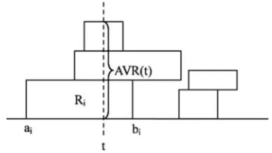
Average Rate Heuristic computes the processor speed as the sum of all available jobs’ average-rate. See Fig. 1. At any time t, processor speed is set to be s(t)=_kdk(t). Then, it uses the

EDF policy to choose among available jobs for execution. Obviously this approach yields a feasible schedule.

Since the analysis of competitive ratio depends on the precise form of P(s), our analysis is conducted under the assumption that P(s)=s2_{. For a given job set J , let OPT(J ) denote} the energy consumption of the optimal schedule, and let AVR(J )=(_kdk(t))2dt denote

the energy consumption of the AVR heuristic schedule. The competitive ratio of the heuristic is defined as the least upper bound of AVR(J )/OPT(J ) over all J .

Fig. 1 Example of AVR heuristic

It has been proved in Yao et al. (1995) that AVR heuristic has a competitive ratio of at most 8 for any job set.

3. Optimal voltage schedule for tree job sets

We consider the scheduling instance when the job intervals are properly nested as in a tree structure. The motivations are twofold: (1) such job sets arise naturally in practice, e.g. in the execution of recursively structured programs; (2) the characterization of the optimal speed function is nontrivial and leads to interesting combinatorial problems of independent interest. 3.1. Characterization of optimal schedule for trees

Definition 2. A job set J is called a tree job set if for any pair of job intervals Ijand Ik, one

of the following relations holds: Ij∩Ik = ∅, Ij ⊆Ikor Ik ⊆Ij.

For a tree job set, the inclusion relationship among job intervals can be represented graph-theoretically by a tree where each node corresponds to a job. See Fig. 2. Job jiis a descendant

of job jkiff Ii⊆Ik; if furthermore no other job jisatisfies Ii⊆Ii⊆Ikthen job jiis a child

of job jk.

Interesting special cases of trees include jobs forming a single path (a nested chain), and jobs sharing a common deadline (or symmetrically, common arrival time). We will present linear algorithms for these cases in the next subsection, after first describing properties and algorithms for the general tree case. As remarked before, it is sufficient to focus on the computation of the optimal speed function s(t); the related function job(t) can be obtained with the EDF principle.

We will prove a key lemma that is central to constructing optimal schedules for tree job sets. Suppose an optimal schedule has been given for a tree job set without its root node, we consider how to update the existing optimal schedule when a root node is added.

Consider any job set J consisting of n jobs (not necessary tree-structured), and an addi-tional new job jn+1with the property that [an+1,bn+1]⊇[ak,bk] for any jk ∈J . We will

show that the optimal schedule s(t) for job set J= J∪ {jn+1}is uniquely determined from the optimal schedule s(t) of J and description of jn+1. That is, information such as [ak,bk]

and Rk for jk ∈J is not needed for computing s(t) from s(t). This property will enable us

to construct the optimal schedule for a tree job set efficiently in a bottom-up procedure. To prove the above claim, we compare the selection of critical intervals for s(t) versus that for s(t). Suppose s(t) consists of m critical intervals I₁∗, . . . ,I_m∗ with lengths l1, . . . ,lm

and speeds s1>· · ·>sm. Comparing the computation of s(t) by Algorithm OS versus

that of s(t), we note that the only new candidate for critical intervals in each round is

In+1=[an+1,bn+1]. (Due to the fact [an+1,bn+1]⊇[ak,bk], no other intervals of the form

[an+1,bk] or [ak,bn+1] is a feasible candidate.) Moreover, as soon as In+1 is selected as the critical interval, all currently remaining jobs will be executed (since their intervals are contained in In+1) and Algorithm OS will terminate.

By examining the intensity g(In+1) of interval In+1 in each round i and comparing it with the speed si, we can determine exactly in which round In+1 will be selected as the critical interval. This index i will be referred to as the terminal index (of job jn+1relative to

s(t)). To find the terminal index i, it is convenient to start with the maximum i=m+1 and search backwards. Let gi(In+1) denote the intensity of In+1as would be calculated in the i -th round of Algorithm OS. Usingwk =sklkto denote the workload executed in the kth critical

interval of s(t) for k=1, . . . ,m, and lettingwm+1=Rn+1and lm+1= |In+1| −

m k=1lk, we

can write gi(In+1) as gi(In+1)=(mk=+i1wk)/( m+1

k=i lk).

It follows that the terminal index is the largest i , 1≤i ≤m+1, for which the following holds: gi(In+1)≥si and gi−1(In+1)<si−1(where we set s0= ∞, g0(In+1)=0, and sm+1= 0 as boundary conditions).

We have proven the following main lemma for tree job sets.

Lemma 1. Let the optimal schedule s(t) for a job set J be given, consisting of speeds s1>· · ·>smover intervals I1∗, . . . ,Im∗. If a new job jn+1satisfies [an+1,bn+1]⊇[ak,bk] for all jk ∈J , then the optimal schedule s(t) for J∪ {jn+1}consists of speeds s1 >s2 >· · ·>si where

(1) i is the terminal index of jn+1relative to s(t),

(2) critical intervals from 1 up to i−1 are identical in s(t) and s(t), and (3) the i -th critical interval for s(t) has speed s_i=gi(In+1) over In+1−

i−1

k=1Ik∗.

A procedure corresponding to the above lemma is given in Algorithm Merge, which updates an optimal schedule when a root node is added. The exact method for finding the terminal index will be discussed in the next subsection. Based on Merge, we obtain a recursive algorithm for finding the optimal schedule for a tree job set as given in Algorithm OST. We also observe the following global property of a tree-induced schedule.

Lemma 2. In the optimal schedule for a tree job set, the execution speeds of jobs along any root-leaf path form a non-decreasing sequence.

Proof: By Lemma 1, for a tree job set Jconsisting of a node jn+1and all of its descendants, the execution speed of jn+1is the minimum among Jsince it defines the last critical interval. The lemma holds by treating every node as the root of some subtree. 3.2. Finding terminal indices for trees

Algorithm 2: Merge

Input: Optimal schedule S for J, new job jn+1

Output: Optimal schedule Sfor J= J∪ {jn+1}

S←S

i←Find(S,jn+1){find terminal index i}

In S, replace si,si+1, . . . ,smwith si=gi(In+1) Return S

Algorithm 3: OST(Optimal Scheduling for Tree) Input: root r of tree job set J

Output: Optimal Schedule SJ for J

Initialize SJ−{r}to be∅ for all Children chkof r do

SJ−{r}←SJ−{r}∪OST(chk) end for

SJ ←Merge(SJ−{r},r )

Return S

Algorithm OST gives a recursive procedure for constructing optimal schedule for a tree job set. The important step is to carry out Merge(SJ−{r},r ) at every node r of the tree by

finding the correct terminal index i . Naively, it would seem that sorting the execution speeds of all of rs descendants is necessary for finding the terminal index quickly. It turns out that

sorting (an O(n log n) process) can be replaced by median-finding (an O(n) process Blum et al. (1973)) as we show next. This enables us to achieve O(P) complexity for the overall algorithm where P is the tree’s total path length. For trees of bounded depth this gives an

O(n) algorithm. In the following discussion, we denote the optimal schedule of job set J as SJ.

Theorem 1. Algorithm OST can compute an optimal schedule for any tree job set in O(P) time where P is the total path length of the tree.

Proof: For every Merge operation, we can find the terminal index by performing a binary

search on the median speed in SJ−r. That is, we find the median speed sk and then decide in

which half to search further. See Algorithm 4. Finding the median of a list of t items costs

O(t) time. Calculation of the associated g(In+1) value is also O(t). The total cost of a binary

search for the terminal index thus amounts to a geometric series whose sum is bounded by

O(t). Therefore, the cost of Merge(SJ−{r},r ) is proportional to the number of descendant

nodes of r . Hence the total cost of Merge over all nodes of the tree is upper bounded by the

Algorithm 4: Find (by Median Search)

Input: Schedule S consisting of speed{s1,s2, . . . ,sm}in unsorted manner, new job jn+1

Output: Index i such that gi(In+1)≥siand gi−1(In+1)<si−1.

s0← ∞

sm+1←0

Find median value sk in S

while k isn’t the terminal index do if gk(In+1)<sk then

S← {sj| j >k,sj ∈S} end if

if gk−1(In+1)≥sk−1then

S← {sj| j <k,sj ∈S} end if

Find median speed skin S end while

Return k

3.3. Finding terminal indices for chains

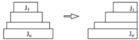
For trees of depth O(n), the above algorithm can have worst case complexity O(n2_). However, we will show that for a nested chain of n jobs (corresponding to a single path of depth n), its optimal schedule can still be computed in O(n) time. Here, instead of using repeated median-finding, Algorithm Merge will keep the speeds sorted and use a linear search to find the terminal index. We note that, without loss of generality, the n nested jobs can be first shifted so they all have a common deadline. (This is because the intersection relationship among time intervals have not been altered.) See Fig. 3. Thus it is sufficient to describe an O(n) algorithm for job sets with a common deadline.

Algorithm 5: Find (by Linear Search)

Input: Schedule S ={s1>s2>· · ·>sm}, new job jn+1

Output: Index i such that gi(In+1)≥siand gi−1(In+1)<si−1.

s0← ∞

sm+1←0

for k=m downto 1 do if gk(In+1)<skthen

Return k+1

end if end for

Fig. 3 Transforming chain job

Theorem 2. The optimal schedule for a job set corresponding to a nested chain can be computed in O(n) time.

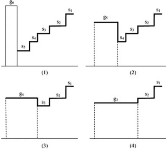
Proof: Let the job intervals be [an+1,b]⊇[an,b]⊇ · · · ⊇[a1,b]. We implement Find(SJ−{jn+1},jn+1) with a linear search for the terminal index, starting with the lowest speed in SJ−{jn+1}. The key observation is that, as can be proven by induction, the speed function s(t) is piecewise increasing from left to right. Hence the search for the terminal index can proceed from left to right, computing gk(In+1) one by one from the smallest sk.

Notice that computing gk(In+1) with knowledge of gk−1(In+1) only costs constant operations.

Furthermore, if we needed to compute g for u consecutive ks before arriving at the right

terminal index, then the total number of critical intervals will also have decreased by u−1. Suppose the Merge operation for the j -th job in the chain (starting from the leaf) computes g for ujtimes, we have

n

k=1(uk−1)≤n, which implies that n

k=1uk ≤2n. Therefore, the

algorithm can finish computing the optimal schedule in O(n) time.

The linear search procedure described above is given in Algorithm 5, and one execution of this Find procedure is illustrated in Fig. 4.

3.4. A weight balancing problem for trees

We have presented two different strategies for implementing the Find operation on trees, as a subroutine used for computing the optimal voltage schedule. We can formulate the problem as a pure weight balancing problem for trees, whose solution will provide alternative algorithms for computing the optimal schedule.

We start with a tree where each node is associated with a pair of weights (wk,lk). The

goal is to adjust the weights so that the ratio sk =wk/lk along any root-leaf path will be

monotonically non-decreasing (see Lemma 2). The rule for modifying the weights is to proceed recursively and, at each node r , ‘merge’ rs weights with those of its descendants

with smallest sk so that their new ‘average’ ratio, as defined by (wk)/lk), will satisfy

the monotonicity condition. The challenge is to find a suitable data structure that supports the selection of rs descendants for the weight balancing . Two different solutions to this problem

were considered in Theorems 1 and 2 respectively. Are there other efficient methods?

Fig. 4 Scheduling of a set of

4. Analysis of competitive ratio

We will analyze the performance of AVR versus OPT for several types of job sets. For convenience of reference, we state the definition of these job sets in the following.

Definition 3. A Job set J is called

(i) a chain job set if a1≤a2≤ · · · ≤anand b1≥b2≥ · · · ≥bn

(ii) a common deadline job set if a1≤a2≤ · · · ≤anand b1=b2= · · · =bn

(iii) a two-overlap job set if Ii∩Ii+2= ∅and a1≤a2≤ · · · ≤anand b1≤b2≤ · · · ≤bn.

4.1. Chain job set

Theorem 3. For any nested chain job set J, AVR(J )≤4 OPT(J ).

This bound of 4 is tight, as an example J provided in Yao et al. (1995) actually achieves

AVR(J )=4 OPT(J ). In this example, the i th job has interval [0,1/n] and density di =

(n/i)3/2_{, this job set has competitive ratio 4 when n→ ∞.}

It is obvious that transforming a chain job set into a common deadline job set by shifting preserves both AVR(J ) and OPT(J ), hence does not affect the competitive ratio. See Fig. 3. Thus we only need to focus on the competitive ratio for the common deadline case. Given a common deadline job set J , the algorithm in Theorem 2 will produce an optimal schedule with exactly one execution interval for each job ji∈J . Denote the execution interval by

[ci,ci+1] where c1=a1, ci ≥aiand cn+1=b. Given J , define Jto be the same as J except

a_i=cifor all i . We call Jthe normalized job set for J .

We make use of the following algebraic relation; its proof is given in the appendix.

Lemma 3. Let X and Xbe two positive constants such that_abX=_abXwhere a≤a≤

b. If Y (t) is a monotone function such that Y (t)≤Y (t) for t≤t, then_ab(X+Y (t))2_≤

b

a(X+Y (t))2+ a

a Y (t)2.

Lemma 4. Given a common deadline job set J , let Jbe the normalized job set for J . Then we have (1) OPT(J )=OPT(J) and (2) AVR(J )≤AVR(J).

Proof: Property (1) is straightforward by the definition of J. Property (2) can be proved by

applying Lemma 3 to the jobs inductively.

Proof of Theorem 3: We first convert J into a common deadline job set. Let Jbe the nor-malized job set for J . By Lemma 4, AVR(J )≤AVR(J) and OPT(J )=OPT(J). According to Theorem 2 in Yao et al. (1995), this will result in a competitive ratio of at most 4 for J.

Combining with AVR(J )≤AVR(J), we obtain AVR(J )≤4 OPT(J ).

4.2. Two-overlap job set

We first consider the simple case of a two-job instance and show that AVR(J )≤1.36 OPT(J ) (the proof is given in the appendix). It is then used as the basis for the n-job case.

Theorem 4. For any two-overlap job set, AVR(J )≤2.72 OPT(J ).

Proof: Denote the two-job instance{ji,ji+1}as Jifor 0≤i≤n. (We also introduce two

empty jobs j0and jn+1.) We have AVR(J )=ni=0AVR(Ji)− n

i=1di2ti. On the other hand,

using the result for two-job sets, we have

n

i=0AVR(Ji)≤1.36

n

i=0OPT(Ji).We observe that any two consecutive jobs in a two-overlap job set must use more energy in the optimal schedule than when they are scheduled alone. Thus,n_i=0OPT(Ji)≤2 OPT(J ).Combining the above three relations, we obtain AVR(J )≤2.72 OPT(J )−n_i=1d2

itiwhich proves the theorem.

5. Lower bound for online schedules

To prove a lower bound on the competitive ratio of all online schedules, we make the as-sumption that the processor time comes in discrete units, i.e. the processor must maintain the same speed over each time unit. Given any online scheduler, we will construct a two-job instance for which the scheduler’s performance is no better than 17₁₃times optimal.

The first job arrives at time 0 and its interval lasts for two time units. Its requirement is two CPU cycles. Suppose the online schedule allocates two CPU cycles to the first job on the first time unit. We then just let the second job be an empty job, and the schedule’s cost is already 2 times optimal.

Suppose the online schedule allocates one CPU cycle to the first job on the first time unit. We construct the second job as follows: it starts from the second time unit and lasts for one time unit and requires 3 CPU cycles. In this case the online schedule’s cost is 17₁₃ times the optimal. This proves that17₁₃is a lower bound on the competitive ratio of all online heuristics.

6. Simulation results

We have simulated the performance of AVR online heuristic in three different types of job sets: general, two-overlap and common deadline job sets. The following data are collected from 1000 randomly generated job sets of each type. Each job set consists of 100 random jobs: the arrival times and deadlines are uniformly distributed over a continuous time interval [0,100] in the general case, and suitably constrained in the other two cases. The required CPU cycles of each job is chosen randomly between 0 and 200.

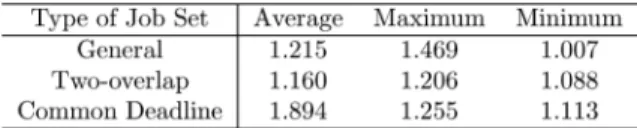
Average, maximum and minimum competitive ratios for each of the three cases are shown in Fig. 5. For the general case, the maximum competitive ratio we observed is 1.47, which is far better than the theoretical bound of 8. The minimum observed ratio is always close to 1. Best among the three, the two-overlap case is where AVR excels, achieving average ratio of 1.16 and maximum ratio of 1.21. For the common deadline case, the maximum ratio encountered of 2.25 is also much better than the bound of 4 proved in Theorem 3.

Fig. 5 Summary of competitive

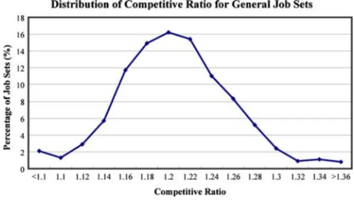
Fig. 6 Simulation result of competitive ratio for general job sets

Fig. 7 Simulation result of competitive ratio for two-overlap job sets

Fig. 8 Simulation result of competitive ratio for common-deadline job sets

The detailed distributions of the competitive ratio obtained from the simulations are give in Figs. 6, 7 and 8. The data suggest that the distributions are close to normal for all three types of job sets, with standard deviations of 0.0528, 0.0162 and 0.1336 respectively.

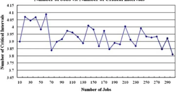
In the second simulation, we look for the growth of the number of critical intervals with respect to the number of jobs in the general case. For each n between 10 and 300, we

Fig. 9 Number of jobs vs. number of critical intervals

randomly generate a set of n jobs, and then compute the average number of critical intervals over 1000 such job sets for each n. Quite surprisingly, this average number does not seem to grow noticeably with the number of jobs. According to Fig. 9, the average number of critical intervals always lies within the range from 3.8 to 4.1 for any n between 10 to 300, with lowest value 3.81 for n=300 and highest value 4.09 for n=60.

7. Conclusion

In this paper, we considered the problem of minimum-energy scheduling for preemptive job sets, under the assumption that energy consumption is a convex function of processor speed. We first focus on the off-line scheduling of tree-structured job sets, where jobs are either properly nested or disjoint. Based on our observation that the optimal execution speeds form a non-decreasing sequence along any root-leaf path in the tree, we derived efficient bottom-up algorithm that computes the optimal voltage schedule for general tree-structured job sets. In addition, we gave an O(n) algorithm for common-deadline or chain job sets.

We also studied the competitive ratio of on-line heuristic AVR for common-deadline job sets and limited-overlap job sets. A tight bound of 4 is proved in the former case, and an upper bound of 2.72 is proved in the latter case. Finally, we established that 17₁₃ is a lower bound on the competitive ratio for any online schedule assuming that time is discrete.

Some interesting open problems remain. Our simulation results suggest that the number of critical intervals grows slowly with n; what exactly is the asymptotic rate? Can our findings for tree-structured job sets be generalized to other classes of job sets? Can the tree case itself be solved even more efficiently?

Appendix Proof of lemma 3:

Proof: After cancelling out identical terms from both sides of the inequality, we are left

to prove_ab(X2_{+2X Y (t))≤}b

a(X

2₊

2XY (t)). The condition_abX=_abXensures that

b a X2≤

b

aX2since X ≤X. Hence it only remains to show

b

a X Y (t)≤ b

aXY (t). Mul-tiplying both sides of_abX=_abXby Y (a) gives us

b

a X Y (a)= b

only need to show_abX (Y (t)−Y (a))≤_abX(Y (t)−Y (a)). But the monotonicity of Y (t) implies that_aaX (Y (t)−Y (a))≤0. Combining with the fact that X≤X, we prove the lemma. If we use X (t) and X(t) to denote the corresponding step functions over [a,b] (by

defining X(t) to be zero over [a,a]), then the above lemma can be written more simply as

b a

(X (t)+Y (t))2≤ b

a

(X(t)+Y (t))2.

Proof of lemma 5:

Proof: We will divide our discussion into two cases according to the number of critical

intervals in the optimal schedule. It’s convenient to define t1=a2−a1, t2=b1−a2and

t3=b2−b1.

Case 1. The two jobs are scheduled in two separate critical intervals. Without loss of

gener-ality, assume the first critical interval is [a2,b2], which implies

d1≤

t1

t1+t2

d2. Thus,

AVR(J )=t1d12+t2(d1+d2)2+t3d22OPT(J )=

d1(t1+t2)

t1

2

t1+(t2+t3)d22 Define f (ρ)= 3√3

(ρ(ρ−1)(2ρ−1))∗(ρ−1).

It can be calculated that f (1.36)>1. This fact, together with two inequalities a+b+c≥

3√3

abc and a+b≥2√ab implies that AVR(J )<1.36 OPT(J ).

Case 2. The two jobs are scheduled in the same critical interval [a1,b2]. Therefore,

t1

t1+t2

d2≤d1≤

t2+t3

t3

d2.

We can normalize the parameters so thatα≤d1, 1−α≤d2and 0≤d1,d2≤1. The cost of optimal schedule becomes 1, while the cost of AVR is

AVR(J )=

α

d1+ 1−α

d2 −

1

(d1+d2)2+

1−1−α

d2

d₁2+

1− α

d1

d₂2

=(d2−d1)α+2d1+d2−2d1d2.

The domain of this function is constrained byα≤d1≤1, 1−α≤d2≤1 and 0≤α≤1. We first calculate the maximum value of AVR(J ) reached in the interior of the domain. At the point where the maximum occurs, the three partial derivatives should all be zero, i.e.

d2−d1=0, 2−α−2d2=0 and 1+α−2d1=0. This impliesα=0.5 and d1=d2= 0.75, which gives us AVR(J )=9

reached on the boundary of the domain is 5₄. Thus, over the entire domain, the maximum value of AVR(J ) is5₄. Summarizing the above two cases, we have shown that for any two-job

job set, AVR(J )≤1.36 OPT(J ).

References

Augustine J, Irani S, Swamy C (2004) Optimal power-down strategies. In: Proc. of the 45th Annual Symposium on Foundations of Computer Science, pp. 530–539

Bansal N, Kimbrel T, Pruhs K (2004) Dynamic speed scaling to manage energy and temperature. In: Proc. of the 45th Annual Symposium on Foundations of Computer Science, pp. 520–529 .

Blum M, Floyd R, Pratt V, Rivest R, Tarjan R (1973) Time bounds for selection. J Comp and Sys Sci 7:488–461 Intel Corporation, Wireless intel speedstep power manager—optimizing power consumption for the intel

PXA27x processor family. Wireless Intel SpeedStep(R) Power Manager White Paper, 2004

Jejurikar R, Gupta RK (2004) Dynamic voltage scaling for systemwide energy minimization in real-time embedded systems. International Symposium on Low Power Electronics and Design

Kwon W, Kim T (2003) Optimal voltage allocation techniques for dynamically variable voltage processors. 40th Design Automation Conference

Mochocki B, Hu XS, Quan G (2002) A realistic variable voltage scheduling model for real-time applications. IEEE/ACM International Conference on Computer-Aided Design

Yao F, Demers A, Shenker S (1995) A scheduling model for reduced cpu energy. In: Proc. of the 36th Annual Symposium on Foundations of Computer Science, 374–382

Yun HS, Kim J (2003) On energy-optimal voltage scheduling for fixed-priority hard real-time systems. ACM Transactions on Embedded Computing Systems 2(3):393–430