Distributions
by Rodney Kreps
ABSTRACT
We model a claims process as a random time to occurrence
followed by a random time to a single payment. Since
ac-cident year payout data available is aggregated by
develop-ment year rather than by paydevelop-ment lag, we calculate those
probabilities and parameterize the payout lag time
distri-bution to maximize the fit to data. General formulae are
given for any distribution, but we use a piecewise linear
continuous distribution.
The companion spreadsheets show the process. It is
sometimes found useful to compromise the quality of the
fit to improve believability of the payout distribution. A
simulation check and example are provided.
As a result, uncertain data can be effectively smoothed
and partial accident year data consistently used.
1. Introduction
We want to consider the model of a claim with a random occurrence time followed by one pay-ment after a random lag time. Our interest is in creating the distribution of payment lag time from occurrence. This distribution could best be estimated by having actual lag data for individ-ual claims and then performing maximum likeli-hood estimation procedures on various distribu-tions. However, actuaries typically do not have such data. Usually they have dollars or counts in the form of accident year by development year or by quarter, and sometimes policy year by de-velopment year. The payout information comes from estimating fractions of ultimate by devel-opment lag from the triangles of data and in-terpreting them as the probabilities of a cumu-lative distribution function. The aggregation of payment data is on the combined occurrence-payment process, which adds the two random times of occurrence and lag-to-payment to get the payout time.
The usual actuarial model of the claims pro-cess is that claims happen in the middle of the year and that payment activity happens only on anniversary dates of the claim; that is, immedi-ately, exactly one year later, exactly two years later, and so on. The virtue of this model of the payout lag time distribution is that accident year by development year payout patterns are easy to fit. The payout density consists of a series of point masses on the anniversary dates, with the probabilities given directly by the aggregated data. Further, unless there are time-sensitive fea-tures in the problem, this may be adequate.
In this paper both the accident date and the lag to payment are modeled as continuous vari-ables. One resulting advantage is that, given the payout lag distribution, we can work with partial years1 or switch to accident year by development quarter, or even accident year by
1See Section A.5 for an example.
development month if desired. It provides a nat-ural way of interpolating empirical payouts and hence development factors. This representation allows one to use partial years of data at ei-ther end or even work with time periods of vari-able length. The technique also gives a consistent smoothing technique for payouts.
Section 2 develops the underlying formulas for arbitrary distribution density functions. Section 3 specializes to the particular class of distribu-tions which are piecewise linear and continuous with a possible mass point at the origin. Details of much of the mathematics are relegated to the appendices.
Section 4 discusses the use of the formulas and the possible desirability of smoothing. The pay-out lag time distribution represents the combined activity of the claims departments, claimants, and sometimes courts. Our preference for the payout lag time density is a smooth curve with no zero values before the final tail.
Section 5 discusses how the companion spreadsheets are set up and how to use them. An example is given which uses excess layer Med-ical Malpractice (Med-Mal) data to illustrate the notions.
2. Probabilities and payouts
We denote byf(t) the probability density func-tion for the lag time t of a payment for a claim occurring at time zero. We have the natural con-dition thatf(t) = 0 fort <0 (a claim is not usu-ally paid before it occurs). Here, we assume that the density function for individual claim payment depends only on the time difference between oc-currence and payment.2
We denote the probability density function for occurrence at time t by occ(t). The occurrence distribution is assumed uniform but the equations
2In principle we could incorporate calendar time as well, if there
could be modified to accommodate seasonality.3 Then the density for payment at time t is the convolution4 of these two densities:
p(t) = Z t
¡1occ(x)f(t¡x)dx: (2.1)
Intuitively, this is the probability of an occur-rence at time x multiplied by the probability of a payment at time t (lag of t¡x), summed over available occurrence times. The probability of a payment between times a and bis
P(a,b) = Z b
a p(t)dt
= Z b
a
½Z t
¡1occ(x)f(t¡x)dx
¾ dt
= Z 1
0
(Z b
a occ(t¡z)dt
)
f(z)dz:
(2.2)
We may now frame the problem as follows: we have developed the probabilities of payment in various intervals (and ideally also their un-certainties5) from some empirical payout pattern. We want to find a density function which is ev-erywhere non-negative and closely gives the em-pirical payout pattern probabilities. We will sup-plement this in Section 4 by requiring that the density function also be reasonably believable.
We want the count payout pattern, but often have only a dollar payout pattern. If severities do not change over time then this is also the count payout pattern. However, it is often felt that larger claims close later, and in such a case we would have to find some way to approximate the count pattern. It may also be that the data is sufficiently noisy that it does not matter.
3The housekeeping would get messy with such modifications
be-cause there would be many points in the year to consider rather than just the endpoints.
4See any book on probability theory, for instanceAn Introduction
to Probability Theory and Its Applicationsby William Feller. 5At the least, if the probabilities result from averaging over accident
years we would want to know the associated standard deviations. The spreadsheet is set up to use relative uncertainties.
For accident-year data we take a uniform oc-currence distribution between times 0 and 1. In Appendix A.2 the probability of seeing a pay-ment in developpay-ment year6n= 0, 1,: : :is derived. Note that development year n begins at time n and ends at time n+ 1.
P(n) = Z n
n¡1(1 +
z¡n)f(z)dz
+ Z n+1
n (n+ 1¡z)f(z)dz: (2.3)
The first term is, of course, missing7 for n= 0. The two terms represent the probabilities for a payment in calendar yearnto come from payout year n¡1 or payout yearn.
An alternative form of Equation (2.3) can be stated by using the cumulative distribution func-tion (cdf)
F(x)´
Z x
0
f(z)dz (2.4)
and the first moment cumulative distribution function
F1(x)´
Z x
0
zf(z)dz: (2.5)
We define the increments
¢(n)´F(n+ 1)¡F(n), and (2.6)
¢1(n)´F1(n+ 1)¡F1(n): (2.7)
We can also recognize that because of the gen-eralized mean value theorem there is a quantity
μn such that 0<μn<1 and
¢1(n) = (n+μn)¢(n): (2.8)
The specific form of μn will depend on the un-derlying density, of course. In Equation (A.16), Appendix A.2 we derive the concise result
P(n) = (1¡μn)¢(n) +μn¡1¢(n¡1): (2.9)
6Partial years or nonyearly intervals sometimes occur in real data;
The equivalent and more directly usable form us-ing cdf increments is
P(n) = (n+ 1)¢(n)¡(n¡1)¢(n¡1)¡¢1(n)
+¢1(n¡1) (2.10)
forn¸1 and
P(0) =¢(0)¡¢1(0): (2.11)
As an example, if the density is exponential f(t) =e¡t=¿=¿ with mean time ¿ >0 then
F(n) = Z n
0
e¡z=¿=¿ dz= 1¡e¡n=¿
¢(n) =e¡n=¿(1¡e¡1=¿)
F1(n) =¿[1¡e¡n=¿(1 +n=¿)] and
¢1(n) =e¡n=¿[(¿+n)(1¡e¡1=¿)¡e¡1=¿]:
For n¸1, P(0) = 1¡¿(1¡e¡1=¿) and P(n) =¿ e¡(n¡1)=¿(1¡e¡1=¿)2. Note that μn=¿¡ (e1=¿¡1)¡1 is independent of n and 0<μn< 1=2, which satisfies the general requirement 0<μn<1.
For accident-year data by development quar-ter, we change the meaning of the index n to refer to quarters. The occurrence distribution is uniform over n= 0, 1, 2, and 3 and a claim has probability 1/4 to be in any one of them. LetQ(n) be the probability for payment from an accident quarter in its development quartern, conditional upon occurrence in that accident quarter. It will have the formulas of Equations (2.9) and (2.10). Let P(n) be the summed accident year by development quarter incremental probabil-ity. Then from Equation (A.21) in Appendix A.3 or just building up the accident year from quarters,
PQ(n) =
n
X
k=max(n¡3,0)
Q(k)=4: (2.12)
The factor 1/4 for each quarter comes from the accident-year occurrence density, as in Equation (A.20).
For policy year by development year, there is an additional step in the process. The policies are written over a year, and we will assume uniform writings, although again it is certainly possible to put in seasonal or other nonuniform behavior. After a policy is written, there is the distribu-tion over time for a claim to happen up to a year later, which again we take to be uniform. The re-sulting claim occurrence density function is tri-angular and extends over two years in Equation (2.2). From Equation (A.25) in Appendix A.4, the probability of a payment in development year nis
PPY(n) = 1 2
Z n+1
n
[(n+ 1)2¡2(n+ 1)z+z2]f(z)dz
+
Z n
n¡1
[1=2¡n(n¡1) + (2n¡1)z¡z2]f(z)dz
+1 2
Z n¡1
n¡2
[(n¡2)2¡2(n¡2)z+z2]f(z)dz:
(2.13)
For n= 0 only the first term is present, and for n= 1 only the first two. We will again express this in terms of the cumulative distribution func-tions, and because there is a quadratic term we will also need the differences of the second mo-ment function:
F2(x)´
Z x
0
z2f(z)dz (2.14)
¢2(n)´F2(n+ 1)¡F2(n)´
Z n+1
n
z2f(z)dz
´(n2+Án)¢(n): (2.15)
The last equality definesÁn. Because of the mean value theorem, 0< Án<2n+ 1 for any distribu-tion. Then we may write
PPY(n) = [1=2¡(n+ 1)μn+ (1=2)Án]¢(n)
+ [1=2 + (2n¡1)μn¡1¡Án¡1]¢(n¡1)
+ [¡(n¡2)μn¡2+ (1=2)Án¡2]¢(n¡2)
or the more directly useful form
PPY(n) =12[(n+ 1)2¢(n)¡2(n+ 1)¢1(n) +¢2(n)]
+f[1=2¡n(n¡1)]¢(n¡1)
+ (2n¡1)¢1(n¡1)¡¢2(n¡1)g
+12[(n¡2)2¢(n¡2)¡2(n¡2)¢1(n¡2)
+¢2(n¡2)] (2.17)
with
PPY(0) = (1=2)[¢(0)¡2¢1(0) +¢2(0)]
PPY(1) = [2¢(1)¡2¢1(1) + (1=2)¢2(1)]
+ [(1=2)¢(0) +¢1(0)¡¢2(0)]:
(2.18)
3. A specific distribution
We will work in the context of the accident-year-by-development-year problem, but the ex-tensions to the other cases are straightforward. The immediate question is how to get the pay-out lag time distribution given a paypay-out pattern. We will pick a parameterized form of the density function and use it to develop formulas for the probabilities. There are, of course, many possible forms and the reader is certainly invited to cre-ate the probabilities of Equation (2.3) from her favorite form.
We will focus on a mixed distribution which has a possible positive probability at zero and a continuous distribution on positive time. A piece-wise linear density function specifies values at the integer8 times and is linear between them. Mathematically, the form is
f(t) =P0±(t) +
N
X
n=0
I[n,n+1](t)
£[(n+ 1¡t)fn+ (t¡n)fn+1]: (3.1)
We have switched from x to t as a variable to remind us that this is the time from occurrence
8If the data came in noninteger intervals, we would adjust the
den-sity intervals.
to payout. The value P0 is the amount of prob-ability9 at t= 0 and is subject to the constraint 0·P0·1. It is meant to represent the probabil-ity of payout immediately after occurrence. The valuesfn are the values of the density function at times t=n. The interval function I[n,n+1](t) is 1 in the interval n·t·n+ 1 and zero otherwise. The density function in that nonzero range has the value
(n+ 1¡t)fn+ (t¡n)fn+1 (3.2)
which yields the straight line from fn at t=n to fn+1 at t=n+ 1. In order to be a probabil-ity densprobabil-ity, we must have fn¸0 for alln. Since our data is always bounded in time, we have specified N+ 1 intervals and we takefn= 0 for n >=N+ 1. However, if the reader knows of a good form for the tail she is encouraged to use it. For some patterns such as workers comp the distribution density almost certainly should be nonzero, well past any data we actually have.
Appendix B derives the results of the rest of this section. The differences of the cdf are
¢(n) = fn+fn+1
2 for n >0 and
¢(0) = f0+f1 2 +P0:
(3.3)
The cdf starts with P0 and is quadratic in each interval. If K is the integer part of tand z is the fractional part oftso thatt=K+zand 0·z <1, then
F(t) =P0+
KX¡1
n=0
fn+fn+1
2 +
z
2[(2¡z)fK+zfK+1]:
(3.4)
IfK= 0 the sum does not contribute. There is a constraint on the fn in that the total probability must be 1:
1 =F(N+ 1) =P0+f0 2 +
N
X
n=1
fn: (3.5)
9The delta function integrates to 1 and is zero for nonzero
The accident-year-by-development-year prob-abilities of Equation (2.9) for n >0 are
P(n) = fn¡1+ 4fn+fn+1
6 : (3.6)
There are some special cases at both ends of the distributions:
P(0) =P0+2f0+f1 6
P(N) = fN¡1+ 4fN 6
P(N+ 1) =fN 6 P(n > N+ 1) = 0:
(3.7)
The accident-year-by-development-quarter probabilities from Equation (2.12) are generally
PQ(n) = fn¡4+ 5fn¡3+ 6fn¡2+ 6fn¡1+ 5fn+fn+1
24 :
(3.8)
The special cases at the start are from Equation (A.21),
PQ(0) = Pr0+ 2f0+f1
24
PQ(1) = Pr0+3f0+5f1+f2 24
PQ(2) = Pr0+
3f0+6f1+5f2+f3
24
PQ(3) = Pr0+
3f0+6f1+6f2+5f3+f4
24 ,
(3.9)
and the special cases at the end are
PQ(N) =fN¡4+ 5fN¡3+ 6fN¡2+ 6fN¡1+ 5fN 24
PQ(N+ 1) =fN¡3+ 5fN¡2+ 6fN¡1+ 6fN 24
PQ(N+ 2) =fN¡2+ 5fN¡1+ 6fN 24
(3.10)
PQ(N+ 3) =fN¡1+ 5fN 24
PQ(N+ 4) =fN 24
PQ(n) = 0 for n > N+ 4:
In practice it is easier just to use Equation (2.12) for the accident year as a sum of quarters.
The policy-year-by-development-year proba-bilities of Equation (2.16) are
PPY(n) = 241 (fn¡2+ 8fn¡1+ 14fn+fn+1):
(3.11) The special cases are similarly at the ends
PPY(0) =Pr0
2 +
3f0+f1 24
PPY(1) =Pr0
2 +
8f0+ 11f1+f2 24
(3.12)
and
PPY(N) = fN¡2+ 8fN¡1+ 14fN 24
PPY(N+ 1) =fN¡1+ 8fN 24
PPY(N+ 2) =fN 24
PPY(n) = 0 for n > N+ 2:
(3.13)
4. Believability and smoothing
It is a fair question to ask why we have both-ered with creating a continuous distribution for payout times. As mentioned in the introduction, the implicit accident-year-by-development-year payout distribution which is widely used is one where the density is nonzero only at a discrete set of points on the lag time axis. The virtue of this distribution is that it is easy to parameterize. If the payout pattern indicates X% of the claims are paid in yearn, then we put a X% probability att=n.
This discrete distribution requires that once a claim occurs, it either is paid immediately or is paid exactly on one of its anniversary dates. While special circumstances may suggest that some claim payments may cluster around an-niversary dates, in general it not believable that claims never have payments at times other than anniversary dates.
the complexity of the process that actually pro-duces a payment. We do not expect that there will be lag times with no probability of payment before the end of the tail.
We are trying to create a distribution over pay-ment lag time that more closely reflects real-ity. We do not know exactly what this distri-bution should look like for any given line of business. The distribution could have a proba-bility of (almost) immediate payment. The den-sity should ultimately fall to zero. For some di-rect lines such as personal insurance, we might expect the density to decrease monotonically to zero. Alternatively, it may have a peak a few years out. For excess lines and reinsurance per-haps the density should rise from zero. There is some suggestion that workers comp claims may be bimodal because of short- and long-term care. Also, there may be enough of a distinction in some lines of business between claims that go to court and those that do not to create more than one peak.
In all cases, we do not expect there to be re-gions of zero probability before the final tailing out and we do expect the density to be smooth– the failure of both these requirements is what we find unreal about the discrete distribution.
What prejudgment on the density may or not be applied to results from available data is clearly a matter for the judgment of the actuary in any particular situation.
There is another reason for considering smoothing, which has to do with the noise in any data. Looking at the accident-year relations Equations (3.6) and (3.7), it would seem that for a finite amount of data we should just solve the equations. We certainly could. After all, we have N+ 2 probabilitiesP(0) toP(N+ 1) and we have N+ 2 parameters in P0 and f0 tofN. It is even a set of linear equations, and we can begin at the high end and work recursively backwards. This sounds good until it comes up against actual data. While it is true that mathematically the equations
can be easily solved, what cannot be guaranteed is that all the parameters thus produced from real data10 are positive. If they aren’t, then we do not have an actual density function and we have to try something different.
Note that negative parameters in the density have nothing to do with negative payments; we are talking about the probabilities of having a payment and not about the payment size. If one has a line with considerable salvage and subro-gation at the end of the payment pattern, it may be worthwhile to have the severity change sign at some point in time or create two densities, one for the positive payments and one for the nega-tive. If the data are separate, just model sal-sub separately from the outgoing payments.
What can create negative parameters? Having data from not very many claims in the payout triangles; using average11 payout values and not recognizing the uncertainty associated with them; not really having a line of business where the payout pattern can be reasonably represented by only a single payment; having noise in the data from miscoding or other sources; any combina-tion of the above; or something else. We do not expect to get negative parameters for payout pat-terns created by many claims in straightforward lines of business, but we want a procedure which will always work.
So what can we do? We can recognize that the data always has noise in it, and that a perfect fit may not even be desirable. Outliers do hap-pen. We can pick some measure of fit–we used variance-weighted least squares error–and min-imize the differences between the data and the predicted probabilities using normalized positive parameters. In other words, we can insist on a proper density function and see how close we can get. In the cases where we could solve the equa-tions and get positive parameters, we will get the
10The author’s experience with high excess layers may have
solution and in every case we have something physically consistent.12
Experimentation with the spreadsheet tools has indicated that it is typically possible to get a pretty good fit, even to very irregular data. How-ever, the cost to the best fit may be that the den-sity function has violent swings in it, and possi-bly be zero over some periods. Neither of these properties is desirable, and we would like to have a way to ameliorate them.
The spreadsheets have as an input the weight to be given to having a smooth result. As this weight is increased from zero, the payout density function gets smoother–here meaning smaller changes in the slopes from segment to segment. However, the fit gets worse. The question of how much weight to give to the smoothing to get a more believable density function is purely sub-jective, and depends in part on how bad it is to be away from the exact values of the data points. If the data points have substantial intrinsic uncer-tainty, then considerable smoothing of the den-sity may be possible with very little statistical loss of fit even though the predicted curve moves substantially.
It should be said that if smoothing is used, the density parameters will depend on the smooth-ness measure as well as on the degree to which the smoothness is imposed. The measure of smoothness used here, which seems to work well, is the sum of the squares of the differences of the slopes at each interior point in the distribu-tion. This measure is zero when the density is a straight line and responds strongly to “W” shapes in the density. The reader is of course invited to use any smoothing measure that seems appropri-ate or none at all if it is not needed.
Since the predicted curve is derived from us-ing a valid density, it smoothes–“graduates” in older terminology–the data in a consistent fash-ion. Frequently smoothing of the data is desirable
12That is, no negative probabilities.
in the first place and was often done on an ad hoc basis.
There is one further consideration. After do-ing the smoothdo-ing or not, the analyst may recog-nize the shape of the density function as being essentially gamma or Pareto or something simi-lar. If so, it is generally preferable to work with fewer rather than more parameters and it would be good to go back and recalculate the proba-bilities in the intervals on the basis of the new form of the density. These calculations are easily done in terms of the cdf and first moment cdf differences with Equation (2.10).
5. Spreadsheet tools
We will work with “AY Payout Density.xls” as the exemplar, since the accident quarter and pol-icy year are similar except for the detailed for-mulas in the probabilities. These differ in that for “AY Payout Density.xls” we use Equations (3.6) and (3.7), while for “AQ Payout Density.xls” we incorporate accident-quarter data via Equation (2.12). This is equivalent to using Equations (3.8) to (3.10) but is perhaps easier to understand. For “PY Payout Density.xls” we use Equations (3.11) to (3.13).
The sheet labeled “accident-year data” has its inputs in light blue. There is an input for the pay-out pattern, its name, and the relative uncertainty of the payouts. The fundamental measure of fit is the square of the difference between the fitted values and the data divided by the square of the uncertainty, and summed over all the data points. There is also an input for the weight to give to smoothing. At first, leave it at zero.
We begin by entering data. The data below is from some excess Med-Mal reinsurance con-tracts, but the uncertainties are estimated. Note that we have put in a relatively larger uncer-tainty for the earlier values.13 The button “Guess Start Values” puts half of the first data value
13This could be the standard deviation of the values used to get the
Figure 1. Data with “Guess Start Values” applied to the density
(at n= 0) into the probability at zero, and puts the probabilities at each n as the estimate for fn. In the other spreadsheets there are modifica-tions from these formulas made to the first few cells.
After clicking on “Guess Start Values” the data sheet “accident year data” looks in part as in Figure 1.
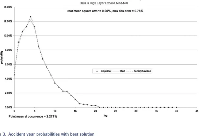
The graph sheet “AY probabilities” then shows Figure 2.
The graph’s horizontal axis has two meanings: for the data and the fit, it is the development period. For the density function, it is the lag from occurrence. At the guessed startup values the density function will follow the payout pat-tern and add a point mass at zero. The fit here is already not too bad.
The next step is to run Excel Solver by click-ing on “Solve.” This will vary all the density
parameters to try to improve the fit. On the spreadsheet, the solver variables are allowed to vary freely, with the positivity constraints being imposed by formula rather in Solver itself. After Solver stops, the graph sheet shows Fig-ure 3.
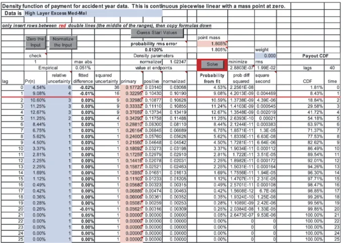
We can see from the error statistics that the fit is better. The root mean square error has de-creased from 0.26% to 0.01% and the maximum absolute error has decreased from 0.76% to 0.05%. One could simply stop here and declare oneself satisfied. The data sheet now shows as in Figure 4.
Some notes for the data sheet: the input ranges can be extended by inserting rows between the two sets of double red lines14 and copying
for-14The second, bottom, set of double red lines is after lag 38 and
Figure 2. Accident Year probabilities with guessed start values
Figure 4. Data sheet with best solution
mulas down. This insures that the special con-ditions at both ends are met and all the named ranges retain their integrity. There are several convenience buttons: “Zero the Input” clears out old input; “Normalize the Input” multiplies it all by a factor to make its sum one; and “Guess Start Values” will usually give a reasonable place to begin the minimizations. As used above, “Solve” will run Excel Solver15 to minimize the crite-rion of fit. The cells in pink, also commented as “solver variable” are parameters changed by Solver.
The column “normalized value at endpoints” is directly thefn of this paper. The column “Prob-ability from fit” is our P(n). The columns la-beled “Payout CDF” are the cdf values of the
15Sometimes Solver will, on the author’s machine, give an error
message. In that case, running the solver once by hand from the menu rather than by the macro from the button seems to fix the problem.
payout density and the corresponding lag time values. If we were working with noninteger time values, then this is where we would make the change, and consequently also on the sheet “CDF draw” to be discussed later. The data sheet gives the minimization function value, the root mean square (RMS) error, and the maximum absolute error for the fit. The latter two are also shown on the graph sheet.
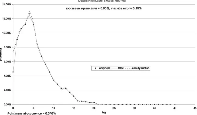
Figure 5. AY probabilities with smoothing 0.001
The recommended use is to start with zero smoothing weight and observe the graph sheet. As you gradually increase the weight the den-sity will become more and more smooth and the fit will worsen. In Figure 3, we might not like the shoulder between lags 2 and 4 and the very high value at lag 5, preferring a smoother vari-ation of the underlying payout density. This is entirely a matter of actuarial judgment. With a smoothing value of 0.001, the graph sheet be-comes as shown in Figure 5. The fit is not par-ticularly worse, and the payout density is much more reasonable to the author’s perspective. It still has a very sharp peak at lag 5 and a wiggle at lags 12 and 13.
If we push the smoothing up to 0.05, we get Figure 6. Whether this fit is unacceptably bad de-pends on what we think the uncertainties are on the data, and especially in this case on how much we really believe the spike in the data at lag 5. This parameterization certainly does smooth out the payout lag time density function. The sugges-tion is to find a compromise that you can believe.
A word of caution: Solver will sometimes hang up in less than optimal solutions. The author’s recommendation is always to start with the “Guess Start Values” and put in the smoothing weight, and then “Solve.”
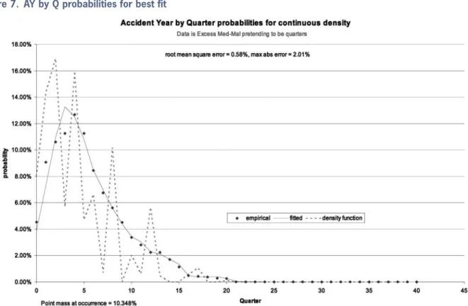
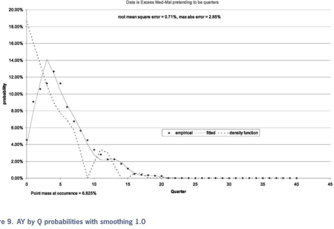
In the spreadsheet “AY by Q payout density. xls” the same accident-year data is used, while pretending that it is quarterly data instead. The best fit shows up as in Figure 7. This is a clear candidate for smoothing. A weight of 0.1 gives Figure 8. This still has zero probability values, so we try a weight of 1, yielding Figure 9. Since the data is unreal, it is perhaps not surprising that much smoothing was required.
Figure 6. AY probabilities with smoothing 0.05
Figure 8. AY by Q probabilities with smoothing 0.1
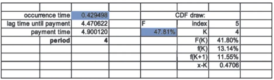
Figure 10. Simulation of a single claim
from the cdf for the lag time from occurrence to payment. These two random times are added together, and then the integer part of their sum is the payment period. If you push F9 (Calcu-late) on this sheet you will see the process. The calculation part of the sheet looks like Figure 10. Again, the shaded cells are random uniform vari-ables from the interval zero to one.
The button “Simulate” on this sheet will erase current data on the sheet “simulation results” and create new data for comparing the simulation with the predicted fit of “Probability from fit.” This is provided in case one wants to validate the formulas, and also is a reminder that a finite number of simulations will usually give a mean result near but not at the theoretical value.
Appendix A. Mathematical
derivations
A.1. Accident-year probabilities
There are undoubtedly much more concise derivations of the results presented here. How-ever, we have used the same methodology ev-erywhere in this appendix and have written this version out in detail so that the reader will hope-fully be able to follow the steps easily.
To aid in deriving Equation (2.3) from a uni-form occurrence distribution and Equation (2.2), we first define the index function and list some of its properties:
£(x) = (
1 for x >0
0 for x <0 )
: (A.1)
This is the unit step function at zero. A useful and intuitive way to read a factor of£(x¡a) is to say
that “xmust be greater thana.” This function has some obvious properties (up to a set of measure zero):
£(x) = 1¡£(¡x): (A.2)
Ifxis greater thanaandxis greater than b, then x is greater than the larger of the two. If a is greater than b, then x is greater than a, but if b is greater thana, then xis greater thanb. Thus
£(x¡a)£(x¡b)
=£(x¡max[a,b])
=£(x¡a)£(a¡b) +£(x¡b)£(b¡a):
(A.3) Similarly, for “less than” relationships,
£(a¡x)£(b¡x) =£(min[a,b]¡x)
=£(a¡x)£(b¡a)
+£(b¡x)£(a¡b) (A.4)
£(x¡a)£(a¡x) = 0 (A.5)
£(x¡a)£(b¡x) =£(x¡a)£(b¡x)£(b¡a):
(A.6)
Equation (A.3) and (A.4) will be particularly use-ful later on in formal manipulation of integrals. In fact, it is often helpful to make all integra-tion limits infinite and put the finite limits into indicator functions. For example, Ra1f(x)dx= R1
¡1£(x¡a)f(x)dx.
We can now state the uniform occurrence time density, which is 1 in the interval 0·t·1 and zero elsewhere, as
A change of variable gives occ(t¡z) =£(t¡z) ¢£(1¡t+z), to be used immediately.
For the accident-year case with b > a using Equation (2.2) the probability for a payment in the interval can be developed. First we state the probability with the index functions:
P(a,b) = Z b
a
½Z 1
0 £(t¡z)£(1¡
t+z)f(z)dz ¾ dt = Z 1 0 (Z b
a £(t¡z)£(1¡
t+z)dt ) f(z)dz = Z 1 0 ½Z 1
¡1£(t¡a)£(b¡t)£(t¡z)
¤£(1 +z¡t)dt ¾
f(z)dz: (A.8)
Then we use Equation (A.3) on £(t¡a)£(t¡z) and Equation (A.4) on the other pair:
P(a,b) = Z 1
0
Z 1
¡1
(
[£(t¡a)£(a¡z) +£(t¡z)£(z¡a)] ¤[£(b¡t)£(1 +z¡b) +£(1 +z¡t)£(b¡1¡z)]
) dt f(z)dz = Z 1 0 Z 1 ¡1 8 > > > > > < > > > > > :
£(t¡a)£(a¡z)£(b¡t)£(1 +z¡b) +£(t¡a)£(a¡z)£(1 +z¡t)£(b¡1¡z)
+£(t¡z)£(z¡a)£(b¡t)£(1 +z¡b) +£(t¡z)£(z¡a)£(1 +z¡t)£(b¡1¡z)
9 > > > > > = > > > > > ;
dt f(z)dz: (A.9)
Finally, integrating outt gives
P(a,b)
= Z 1 0 8 > > > > < > > > > :
(b¡a)£(a¡z)£(1 +z¡b)
+(1 +z¡a)£(1 +z¡a)£(a¡z)£(b¡1¡z)
+(b¡z)£(b¡z)£(z¡a)£(1 +z¡b)
+£(z¡a)£(b¡1¡z)
9 > > > > = > > > > ;
f(z)dz
(A.10)
This is the form that can be used for nonintegral or varying-sized time periods. See Section A.5 for an example where the last period is in-complete. In fact, we can use it for any set of time intervals over which the data happen to be stated.
A.2. Accident year by development year
Herea=n andb=n+ 1 so the probability of payment in lagn¸1 is
P(n) =
Z 1 0 8 > > > > < > > > > :
£(n¡z)£(z¡n)
+(1 +z¡n)£(1 +z¡n)£(n¡z)£(n¡z)
+(n+ 1¡z)£(n+ 1¡z)£(z¡n)£(z¡n)
+£(z¡n)£(n¡z)
9 > > > > = > > > > ;
f(z)dz
=
Z 1
0
½ (1 +z¡n)£(1 +z¡n)£(n¡z)
+(n+ 1¡z)£(n+ 1¡z)£(z¡n)
¾
f(z)dz:
(A.11)
The first and last terms are zero because of Equa-tion (A.5). Finally,
P(n) = Z n
n¡1(1 +
z¡n)f(z)dz
+ Z n+1
n (n+ 1¡z)f(z)dz: (A.12)
This is Equation (2.3). For the first lag, n= 0, only the second term contributes:
P(0) = Z 1
0
(1¡z)f(z)dz: (A.13)
In order to formulate in terms of the cumula-tive distribution functions F(x)´R0xf(z)dz and F1(x)´R0xzf(z)dz, we repeat the definitions in Equations (2.6) to (2.8):
¢(n)´F(n+ 1)¡F(n): (A.14)
¢1(n)´F1(n+ 1)¡F1(n)´(n+μn)¢(n):
(A.15)
We can restate Equation (A.12) forn¸1 as
P(n) = (1¡n)[F(n)¡F(n¡1)] + [F1(n)¡F1(n¡1)]
+ (n+ 1)[F(n+ 1)¡F(n)]¡[F1(n+ 1)¡F1(n)]
= (1¡n)¢(n¡1) +¢1(n¡1) + (n+ 1)¢(n)¡¢1(n):
(A.16)
This is Equation (2.10). This can also be written
P(n) = (1¡n)¢(n¡1) + (n¡1 +μn¡1)¢(n¡1)
+ (n+ 1)¢(n)¡(n+μn)¢(n)
=μn¡1¢(n¡1) + (1¡μn)¢(n): (A.17)
This is Equation (2.9). When n= 0,
P(0) =F(1)¡F1(1) =¢(0)¡μ0¢(0)
= (1¡μ0)¢(0): (A.18)
A.3. Accident year by development
quarter
The index is now taken to mean the quarter. The accident-year occurrence density is uniform in the range 0·t·4 and must integrate to 1, so we have
occ(t) = (1=4)£(t)£(4¡t)
= (1=4) 3
X
n=0
£(t¡n)£(n+ 1¡t):
(A.19)
The second form simply expresses that the acci-dent year is a sum of four acciacci-dent quarters. Let Q(n) be the probability for payment in a quarter by one accident quarter. The formulas are either of Equations (A.12) or (A.16). Let PQ(n) be the summed accident year by development quarter
incremental probability. Then, using the second form of Equation (A.19), we see that we have Equation (2.12):
PQ(n) =
n
X
k=max(n¡3,0)
Q(k)=4: (A.20)
Another way of writing this is to show the first three explicitly, which also shows the growth of the accident year:
PQ(0) =Q(0)=4
PQ(1) = (Q(0) +Q(1))=4
PQ(2) = (Q(0) +Q(1) +Q(2))=4
PQ(n¸3) = n
X
k=n¡3
Q(k)=4:
(A.21)
A.4. Policy year by development year
In order to get the probability of claim occur-rence as a function of time, we need to specify how policies are written and how claims occur for a policy. Let w(t) be the probability density for writing a policy at time tand h(t) the proba-bility density for a claim to happen at timetfrom the onset of the policy. We explicitly assume that h(t) does not depend on the policy issuance time. We also assume that the policies are written uni-formly in the year, and that the probability of a claim occurrence is uniform in the policy period. If other conditions are known, then they can be incorporated into the convolution. Using Equa-tions (A.3) and (A.4) produces
occ(t) =
Z t
¡1
w(x)h(t¡x)dx
=
Z 1
¡1
£(x)£(1¡x)£(t¡x)£(x+ 1¡t)dx
=
Z 1
¡1 (
[£(x)£(1¡t) +£(x+ 1¡t)£(t¡1)]
¤[£(1¡x)£(t¡1) +£(t¡x)£(1¡t)]
) dx
=£(1¡t)
Z 1
¡1
£(x)£(t¡x)dx
+£(t¡1)
Z 1
¡1
£(1¡x)£(x+ 1¡t)dx
This result is the familiar triangular exposure curve rising from zero at t= 0 to 1 at t= 1 and falling to zero again at t= 2.
The probability for payment at time tbetween t=n and t=n+ 1 is again given by Equation (2.2).
PPY(n) =
Z 1
0
½Z n+1
n
o(t¡z)dt ¾
f(z)dz=
Z 1
0 Z 1
¡1
fo(t¡z)£(t¡n)£(n+ 1¡t)gdt f(z)dz
= Z 1 0 Z 1 ¡1 8 > > > > > < > > > > > :
(t¡z)[£(t¡z)£(z¡n) +£(t¡n)£(n¡z)]
¤[£(n+ 1¡t)£(z¡n) +£(1 +z¡t)£(n¡z)]
+(2¡t+z)[£(t¡z¡1)£(z+ 1¡n) +£(t¡n)£(n¡1¡z)]
¤[£(n+ 1¡t)£(z+ 1¡n) +£(2 +z¡t)£(n¡1¡z)]
9 > > > > > = > > > > > ;
dt f(z)dz
= Z 1 0 Z 1 ¡1 8 > > > < > > > :
(t¡z)
"
£(n+ 1¡t)£(t¡z)£(z¡n)
+£(1 +z¡t)£(t¡n)£(n¡z)
#
+(2¡t+z)
"
£(n+ 1¡t)£(t¡z¡1)£(z+ 1¡n)
+£(2 +z¡t)£(t¡n)£(n¡1¡z)
# 9 > > > = > > > ;
dt f(z)dz
= Z 1 0 Z 1 ¡1 t 8 > > > > > < > > > > > :
£(n+ 1¡z¡t)£(t)£(z¡n)
+£(1¡t)£(t¡n+z)£(n¡z)
+£(t+n¡z¡1)£(1¡t)£(z+ 1¡n)
+£(t)£(z+ 2¡n¡t)£(n¡1¡z)
9 > > > > > = > > > > > ;
dt f(z)dz: (A.23)
Integration overtyields the following quadratics:
PPY(n)
= Z 1 0 8 > > > > > > > > > > < > > > > > > > > > > :
£(z¡n)£(n+ 1¡z)(n+ 1¡z)2=2
+£(n¡z)£(1¡n+z)
·
1¡(n¡z)2 2
¸
+£(z+ 1¡n)£(n¡z)
·
1¡(z+ 1¡n)2 2
¸
+£(n¡1¡z)£(2 +z¡n)
·
(2 +z¡n)2 2 ¸ 9 > > > > > > > > > > = > > > > > > > > > > ;
f(z)dz
=1 2
Z n+1
n
(n+ 1¡z)2f(z)dz+1 2
Z n
n¡1
[1¡(n¡z)2]f(z)dz
+1 2
Z n
n¡1
[1¡(z+ 1¡n)2]f(z)dz+1 2
Z n¡1
n¡2
(2 +z¡n)2f(z)dz:
(A.24)
By combining the middle terms we finally have Equation (2.13):
PPY(n) =1 2
Z n+1
n
[(n+ 1)2¡2(n+ 1)z+z2]f(z)dz
+
Z n
n¡1
[1=2¡n(n¡1) + (2n¡1)z¡z2]f(z)dz
+1 2
Z n¡1
n¡2
[(n¡2)2¡2(n¡2)z+z2]f(z)dz: (A.25)
For n= 0 only the first term is present, and for n= 1 only the first two.
Alternatively, we can restate the arguments of the density:
PPY(n) =1 2
Z 1
0
fx2[f(n+ 1
¡x) +f(n¡2 +x)]
+ (1¡x2)[f(n¡x) +f(n¡1 +x)]gdx:
(A.26) Using Equation (A.25),
PPY(n)
=1 2[(n+ 1)
2¢(n)¡2(n+ 1)¢
1(n) +¢2(n)]
+f[1=2¡n(n¡1)]¢(n¡1)
+ (2n¡1)¢1(n¡1)¡¢2(n¡1)g
+1 2[(n¡2)
2¢(n
¡2)¡2(n¡2)¢1(n¡2) +¢2(n¡2)]
where
¢2(n)´F2(n+ 1)¡F2(n)
´
Z n+1
n
z2f(z)dz´(n2+Án)¢(n):
(A.28)
The last form definesÁn, and if we use the earlier mean value variables then
PPY(n) =12[(n+ 1) 2
¡2(n+ 1)(n+μn) + (n
2+Á
n)]¢(n)
+f[1=2¡n(n¡1)] + (2n¡1)(n¡1 +μn¡1)
¡((n¡1)2+Á
n¡1)g¢(n¡1)
+1 2[(n¡2)
2¡2(n¡2)(n¡2 +μ
n¡2)
+ ((n¡2)2+Án¡2)]¢(n¡2)
= [1=2¡(n+ 1)μn+ 1=2Án]¢(n)
+ [1=2 + (2n¡1)μn¡1¡Án¡1]¢(n¡1)
+ [¡(n¡2)μn¡2+ 1=2Án¡2]¢(n¡2): (A.29)
This is Equation (2.16).
A.5. Accident year by development year
with partial last year
This is the situation of A.2 when the last year is incomplete. For example, if we have calendar data as of June 1 there would only be five months of data in the last period of every accident year in a development triangle. A crude adjustment is to multiply the last numbers by 12/5 but in general this is not accurate. We shall take the partial year fraction to betf with 0< tf<1 and we want the probabilities for each of the intervals n·t·n+tf for all n. From Equation (A.10), if n¸1
P(n,n+tf) = Z 1
0
8 > > > > > < > > > > > :
tf£(n¡z)£(1 +z¡n¡tf)
+(1 +z¡n)£(1 +z¡n)£(n¡z)£(n+tf¡1¡z) +(n+tf¡z)£(n+tf¡z)£(z¡n)£(1 +z¡n¡tf)
+£(z¡n)£(n+tf¡1¡z)
9 > > > > > = > > > > > ;
f(z)dz
=tf Z n
n¡1+tf
f(z)dz+
Z n¡1+tf
n¡1
(1¡n+z)f(z)dz+ Z n+tf
n
(n+tf¡z)f(z)dz, (A.30) and
P(0,tf) = Z tf
0 (tf¡z)f(z)dz: (A.31) In terms of the cumulative distribution func-tions, ifn¸1
P(n,n+tf)
=tf[F(n)¡F(n¡1 +tf)]
+ (n+tf)[F(n+tf)¡F(n)]
¡(n¡1)[F(n¡1 +tf)¡F(n¡1)]
¡[F1(n+tf)¡F1(n)] + [F1(n¡1 +tf)¡F1(n¡1)]:
(A.32)
Notice that as tf!1 we recover the result in section A.2.
Appendix B. The piecewise linear
continuous distribution
The general form of a piecewise linear con-tinuous distribution would have an arbitrary set of locations at which the value of the density is specified, and between which the density is linear. There could also be one or more point masses of probability at selected points. The only substantial conditions are that it be everywhere non-negative and that the integral over it is one. For some problems involving partial years, this may be a preferable way to state the problem. The algebra is only a little messier.
the interval function into the index function
f(t) =P0±(t) +
N
X
n=0
£(n+ 1¡t)£(t¡n)
£[(n+ 1¡t)fn+ (t¡n)fn+1]: (B.1)
For tsuch that n·t·n+ 1 the density is linear with value
(n+ 1¡t)fn+ (t¡n)fn+1 (B.2)
running fromfnatt=ntofn+1att=n+ 1. There is the additional point mass att= 0. We typically will take fN+1= 0 so that the density drops to zero in the last interval and is continuous.
In the interest of those who may wish to work with nonidentical periods, we can assume a set of timesT0,T1,T2,: : :at which we specify the density values. The density corresponding to Equation (B.1) is
f(t) =P0±(T0) +
N
X
n=0
£(Tn+1¡t)£(t¡Tn)
£(Tn+1¡t)fn+ (t¡Tn)fn+1
Tn+1¡Tn : (B.3) The usual understanding would be that f(t) = 0 for t < T0. Some of the following case-specific results still hold, such as Equations (B.4) and (B.5); others, such as Equation (B.6), need mod-ification in an obvious fashion where t=TK+ (TK+1¡TK)z. However, the real problem lies in getting the probabilities for the intervals in the general case. Specifically, we need terms such as the integral fromTn¡1 (because we integrate over a year) to Tn and there can be arbitrarily many time points Tm in this range. The two spe-cial cases of most interest are more amenable, though, being where the first or last interval is short.
Returning to the usual case of unit intervals, in all intervals except the first,
¢(n) =
Z n+1
n
f(t)dt=
Z n+1
n
[(n+ 1¡t)fn+ (t¡n)fn+1]dt
=
Z 1
0
[(1¡z)fn+zfn+1]dz=
fn+fn+1
2 :
(B.4)
In the first interval, there is an additional contri-bution from the point mass at zero:
¢(0) = Pr0+ f0+f1
2 : (B.5)
The cdf is piecewise quadratic. Specifically, if t=K+zwith K an integer and 0·z <1 then
F(t) =P0+
Z t
0 f(¿)d¿
=p0+
Z K
0
f(¿)d¿+
Z K+z
K
f(¿)d¿
=P0+ K¡1
X
n=0 ¢(n) +
Z z
0
[(1¡x)fK+xfK+1]dx
=P0+ K¡1
X
n=0
fn+fn+1
2 +
μ z¡z
2
2
¶ fK+z
2
2fK+1
=P0+ K¡1
X
n=0
fn+fn+1
2 +
z
2[(2¡z)fK+zfK+1]:
(B.6)
In the first time interval where t <1 then K= 0 and the sum from n= 0 to n=K¡1 is not present. The normalization condition is that
1 =F(1) =P0+f0 2 +
1
X
n=1
fn (B.7)
and for the case of a finite number of terms, as in Equation (B.1),
1 =F(N+ 1) =P0+f0 2 +
N
X
n=1
fn: (B.8)
We have used the condition fN+1= 0 to get this, as there is really a term with fN+1=2 present in Equation (B.6).
The first moment differences are
¢1(n) = Z n+1
n
tf(t)dt
= Z n+1
n
t[(n+ 1¡t)fn+ (t¡n)fn+1]dt
= Z 1
0 (n+z)[(1¡z)fn+
zfn+1]dz
=n¢(n) +³12¡1 3
´
fn+13fn+1
=3n+ 1 6 fn+
3n+ 2
There is no special form for n= 0 because the point mass is at zero. Remembering Equation (2.8) which defines¢1(n)´(n+μn)¢(n) yields
μn¢(n) = fn+ 2fn+1
6 : (B.10)
We note in passing that
μn=fn+ 2fn+1
6¢(n) =
1 3
fn+ 2fn+1
fn+fn+1 (B.11)
always satisfies 1=3·μn·2=3, a more restric-tive condition than the general result 0<μn<1. Now Equation (B.10) can be used, for exam-ple, in the accident-year probabilities of Equation (A.16) to give
P(n) =μn¡1¢(n¡1) + (1¡μn)¢(n)
= fn¡1+ 2fn
6 +
fn+fn+1
2 ¡
fn+ 2fn+1 6
= fn¡1+ 4fn+fn+1
6 : (B.12)
For n= 0 this becomes
P(0) = (1¡μ0)¢(0) = Pr0+ f0+f1
2 ¡
f0+ 2f1 6
= Pr0+
2f0+f1
6 : (B.13)
As a consequence of our finite case,fn= 0n >= N+ 1 and the last probabilities are
P(N) = fN¡1+ 4fN
6 , P(N+ 1) =
fN 6
(B.14) P(n) = 0 for n > N+ 1:
We can also note that the sum of the probabili-ties equals the sum in the normalization condi-tion Equacondi-tion (B.8), so that if the probabilities sum to 1 the normalization is correct when these equations are solved.
For policy year, we need the second moment differences. In this situation,
¢2(n) = Z n+1
n
t2f(t)dt
= Z n+1
n
t2[(n+ 1¡t)fn+ (t¡n)fn+1]dt
= Z 1
0 (n+z) 2
[(1¡z) +zfn+1]dz
=n2 ·μ
1¡1 2 
fn+1 2fn+1
¸ + 2n ·μ1 2¡ 1 3 
fn+1 3fn+1
¸ + μ1 3¡ 1 4 ¶ fn+1
4fn+1
=n2fn+fn+1
2 +n
fn+ 2fn+1
3 +
fn+ 3fn+1
12 :
(B.15)
Remembering the definition in Equation (A.28) that ¢2(n)´(n2+Án)¢(n),
Án¢(n) =4n+ 1 12 fn+
8n+ 3
12 fn+1: (B.16)
The policy-year probabilities of Equation (2.16) are now
PPY(n) = [1=2¡(n+ 1)μn+ 1=2Án]¢(n) + [1=2 + (2n¡1)μn¡1¡Án¡1]¢(n¡1)
+ [¡(n¡2)μn¡2+ 1=2Án¡2]¢(n¡2)
= ·f
n+fn+1
4 ¡(n+ 1)
fn+ 2fn+1
6 +
4n+ 1 24 fn+
8n+ 3 24 fn+1
¸
+ ·f
n¡1+fn
4 + (2n¡1)
fn¡1+ 2fn
6 ¡
4(n¡1) + 1 12 fn¡1¡
8(n¡1) + 3
12 fn
¸
+ ·
¡(n¡2)fn¡2+ 2fn¡1
6 +
4(n¡2) + 1 24 fn¡2+
8(n¡2) + 3 24 fn¡1
¸
And finally, the policy year probabilities are given by
PPY(n) = 241 (fn¡2+ 8fn¡1+ 14fn+fn+1):
(B.18)
The special cases are the consequences offn= 0 forn >=N+ 1 and the point mass at the origin:
PPY(0) = [1=2¡μ0+ 1=2Á0]¢(0)
=P0 2 +
3f0+f1 24
PPY(1) = [1=2¡2μ1+ 1=2Á1]¢(1)
+ [1=2 +μ0¡Á0]¢(0)
=P0 2 +
8f0+ 11f1+f2
24 : (B.19)
Again, the sum of the probabilities is the right-hand side of the normalization equation, so that if these equations are solved, normalization is au-tomatic.
The last piece we want is the inversion of the cdf of Equation (B.6). We need this in order to do simulations. We start by generating a uniform random variable U with 0< U <1. We want to findt=F¡1(U). We first find the integerK such that
P0+
KX¡1
n=0
fn+fn+1
2 < U·P0+
K
X
n=0
fn+fn+1
2 :
(B.20)
If 0< U·P0, then t=F¡1(U) = 0 and K= 0 when 0< U¡P0·(f0+f1)=2. Because of the normalization condition Equation (B.8), there will always be a value ofK found. We will write
t=K+¢t (B.21)
and solve for ¢t in terms of
¢U´U¡ 8 < :P0+
KX¡1
n=0
fn+fn+1 2
9 =
;: (B.22)
Again, the sum does not exist for K= 0. Refer-ring back to Equation (B.6) we see that
¢U=fK¢t+fK+1¡fK
2 ¢t
2:
(B.23)
The quadratic is elementary, but it is helpful to get the correct root of the equation and elimi-nate any problems when the coefficient of the quadratic term vanishes by writing the solution as
¢t= 2¢U
fK+qf2
K+ 2¢U(fK+1¡fK)
: