41
Wavelet Transform and Autoregressive Integrated
Moving Average Combination Approach in Crude Oil
Prices Forecasting
Nurull Qurraisha Nadiyya Md-Khair, Ruhaidah
Samsudin
Department of Software Engineering, Faculty of Computing Universiti Teknologi Malaysia
81310 Johor Bahru, Johor, Malaysia [email protected], [email protected]
Ani Shabri
Department of Science Mathematics, Faculty of Science Universiti Teknologi Malaysia
81310 Johor Bahru, Johor, Malaysia [email protected]
Submitted: 1/02/2018. Revised edition: 16/05/2018. Accepted: 21/05/2018. Published online: 31/05/2018
Abstract—This paper proposes a time series forecasting approach combining wavelet transform and autoregressive integrated moving average (ARIMA) to enhance the precision in forecasting crude oil spot prices series. Wavelet transform splits the original prices series into several subseries, then the most appropriate model of ARIMA is established to predict each respective series and finally all series are combined back to get the original series. The datasets for the experiment consist of crude oil spot prices from Brent North Sea (Brent) and West Texas Intermediate (WTI). Single forecasting model ARIMA and several existing forecasting approaches in the literatures are used to measure the performance of the proposed approach by utilizing the Mean Absolute Error (MAE) and Root Mean Square Error (RMSE) collected. Final results have depicted that the proposed approach outperforms other approaches with smaller MAE and RMSE values. Ultimately, it is proven that data decomposition, combined with forecasting method can increase the accuracy in time series forecasting.
Keywords—Autoregressive Integrated Moving Average, Wavelet Transform, Hybrid Forecasting Method, Crude Oil Spot Prices, Price Forecast
I.INTRODUCTION
Crude oil price acts as a major part in worldwide economy and its fluctuation is one of vital interests for the market
participants and financial practitioners [1]. It is widely utilized in almost all goods manufacturing at various stages of their production and provides over two-thirds of the world’s energies [2]. Therefore, changes in crude oil prices can influence the global economic activities significantly [3]. For example, the rise in crude oil price would significantly affect the petrol price, thus giving side effect on the fundamental goods and services needed by the citizen. On one hand, a sudden rise in crude oil prices would undesirably bring bad impact on the economic development and hasten inflation in many oil importing countries [4]. Contrarily, a hard dip in crude oil prices would spark a severe economic deficit issues for countries that export oil [5]. Therefore, the understanding of petroleum markets is very important. One way of doing so is to use forecasting methods that are proposed and proven by many studies.
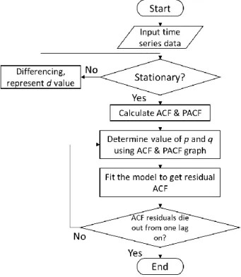
42 Autoregressive integrated moving average (ARIMA) is a very popular method which can be applied in forecasting time series data. It is derived from the single models autoregressive (AR), the moving average (MA) and the consolidation of AR and MA named ARMA model [9]. For data series that is stationary, ARMA model is utilized. However, if the data series is identified to be non-stationary, it is converted to become stationary using ARIMA. ARIMA model is generally represented by the value (𝑝, 𝑑, 𝑞). 𝑝 defines the autoregressive number and 𝑞defines the moving average number. 𝑑 value is the one that differentiates ARIMA model and ARMA model. It denotes the difference order for non-stationary time series. The ARIMA modelling introduced by Box and Jenkins shall comply with the three basic steps. The first step is (1) to identify the suitable model. After an appropriate model is determined, the next step is (2) to perform the parameters estimation. The last step is (3) to validate the model where examination is done to inspect whether the model fits the data adequately.
Many methods have been applied in Crude Oil Spot Prices (COSP) series forecasting. One of the single methods is ARIMA method which is utilized to predict the monthly production of crude oil in Malaysia [10]. Their empirical study claimed that their model of (1,0,0) can be used to obtain future forecasts. One of the problems in single forecasting methods is that most of them can only produce satisfactory prediction when the data series is linear or near linear [1]. The COSP series contains volatility, non-linearity, and irregularity. Therefore, using this dataset on single forecasting methods can decrease the forecasting accuracy.
Besides the single forecasting model stated earlier, researchers also proposed hybrid methods using data decomposition to improve forecasting accuracy and to cater the problems identified in single forecasting methods. An example of hybrid method used in forecasting COSP series is the integration of ensemble empirical mode decomposition (EEMD), generalized autoregressive conditional heteroskedasticity (GARCH) and least square support vector machine with particle swarm optimization (LSSVM–PSO) [11]. The proposed method is proven to be effective in assisting investors and analysts to assess the moving trends of COSP series. Another hybrid method used in forecasting COSP series is based on empirical mode decomposition (EMD) which is applied for decomposition, feed-forward neural network (FNN) which is utilized for prediction and adaptive linear neural network (ALNN) which is used for assembling [4]. Based on their experiment, they conclude that their proposed hybrid method which incorporates data decomposition has managed to perform better than the other comparative methods.
In this study, a combination approach of wavelet transform and ARIMA that can enhance the efficacy of COSP series forecasting is proposed. Firstly, wavelet transform is applied to the original COSP series to produce several distinct subseries. Next, an appropriate ARIMA model is constructed and applied for each subseries. Lastly, forecasting output obtained from all subseries are combined and converted to become the forecasted original COSP series using inverse wavelet transform. For empirical study purpose, the data of crude oil spot prices market from Brent North Sea (Brent) and West Texas Intermediate (WTI) are collected as datasets. To appraise the efficacy of the
proposed approach, single forecasting model ARIMA and several existing approaches that forecast COSP in the literatures are used for comparison. The comparison is analysed using Mean Absolute Error (MAE) and Root Mean Square Error (RMSE) acquired from each approach. The rest of the paper is structured as follows. Section II presents the methodologies involved in this paper which include clarification about the dataset used, ARIMA model, wavelet transform, the proposed approach and effectiveness assessment criteria. Then, the experiment result and analysis are discussed in Section III. Eventually, Section IV concludes the study.
II.METHODOLOGY
A.Crude Oil Spot Prices Dataset
The COSP series datasets used in this empirical study were acquired from the website of U.S. Energy Information Administration that grants public access to datasets for various renewable and non-renewable energy sources [12]. WTI, also known as Texas light weight is a grade of crude oil used in benchmarking oil prices. WTI grade is defined as light and sweet because it is low in density and sulfuric content which is 0.24 percent. Since WTI crude oil is high in quality and is produced within the Midwest and Gulf Coast regions in the U.S, it is refined mostly in those regions. On the other hand, Brent grade also serves as a major benchmark oil price for worldwide oil purchases. Brent grade contains approximately 0.37 percent of sulphur and is considered as light and sweet, similar to WTI. Brent grade is typically refined in Northwest Europe and is applicable in petrol and middle distillates production. For the experiment, daily COSP from Brent and WTI starting from January 2000 until November 2016 were utilized. Both datasets of WTI and Brent consist of 4228 and 4274 daily observations respectively.
B.Discrete Wavelet Transform
Time series data normally exhibits variance that is not constant and mean with considerable outliers which makes prediction challenging [13]. In such case, wavelet transform breaks down time series data into approximation components and details components. Consequently, prediction result would be more accurate because the variance and mean of the time series data become more consistent. Some of the following wavelet transform equations are extracted from the research done by Kriechbaumer et al. [8]. A mother (𝜓) wavelet derives each wavelet family by expansion and translation to generate daughter wavelets 𝜓𝑢,𝑠(𝑡). The equation is expressed as below,
𝜓𝑢,𝑠(𝑡) =
1
√𝑠𝜓 ( 𝑡 − 𝑢
𝑠 ) (1)
43 function. For instance, the shape of a Haar wavelet is symmetric, square shaped and discrete, Daubechies has asymmetric shape while Symlet and Coiflet have symmetric shapes. The “order” of a mother wavelet will determine its width [6]. The selection of the “order” is usually determined by the smoothness of the time series itself [8].
By using wavelet transform, a time series is displayed in its time-frequency representation that results in coefficients of wavelet. There are three types of wavelet transform that can be identified depending on the generated number of coefficients. They are discrete wavelet transform (DWT), continuous wavelet transform (CWT) and maximum overlap DWT (MODWT). DWT is chosen because it involves short computation time and is more straightforward to apply compared to CWT and MODWT [1]. By using DWT, only essential coefficients needed to rebuild the original function 𝑥(𝑡) are generated. To gain this downsizing, the parameters s
and u are discretized to become 𝑠 = 2−𝑗 and 𝑢 = 𝑘2−𝑗where k
and j are integers. j describes the particular decomposition level where 𝑗 = 1, … , 𝐽 and J represents the number of decomposition levels created. The selection of a wavelet function and number of decomposition level depends on the frequency and type of variations the analyst intends to capture in a time series [8]. The following formula can be utilized to assist in finding the suitable number of decomposition level for a particular time series data where 𝐿 represents the decomposition level and 𝑁 represents the total amount of observations in a time series data [14].
𝐿 = 𝑖𝑛𝑡[𝑙𝑜𝑔(𝑁)] (2)
Based on multiresolution analysis (MRA), wavelet transform is employed to divide the time series into a smooth series 𝐴𝐽
that contains smooth coefficients 𝑎𝐽,𝑘, and a group of detail
series 𝐷𝑗 that contains detail coefficients 𝑑𝑗,𝑘. The smooth
series, portrayed as a de-noised form of the original time series is the essential part of MRA [6]. Meanwhile, the detail series apprehends the fluctuations around the smooth series. Lastly, original series is reconstructed by adding up the coefficients of detail series 𝐷𝑗 with the smooth series 𝐴𝐽 using the subsequent
equation:
𝑥𝑡= ∑ 𝑎𝐽,𝑡 𝐽
𝑗=1
+ 𝑑𝑗,𝑡 (3)
C.Autoregressive Integrated Moving Average
ARIMA is a very popular model when it comes to predicting time series. It is a combination of AR model, MA model and the integration of AR and MA known as ARMA model. In AR model of order p, AR(𝑝), the typical formula to indicate the prevailing value of time series is as follows:
𝑦𝑡= 𝜙1𝑦𝑡−1+ 𝜙2𝑦𝑡−2+ ⋯ + 𝜙𝑝𝑦𝑡−𝑝+ 𝜀𝑡 (4)
The prevailing value of a time series as a current and 𝑞 past values of random errors that is indicated by the MA(𝑞) can be formulated as:
𝑦𝑡= 𝜀𝑡− 𝜃1𝜀𝑡−1− 𝜃2𝜀𝑡−2− ⋯ − 𝜃𝑞𝜀𝑡−𝑞 (5)
Therefore, the generic expression for a merged ARMA (𝑝, 𝑞) operation can be described as:
𝑦𝑡= 𝜙1𝑦𝑡−1+ 𝜙2𝑦𝑡−2+ ⋯ + 𝜙𝑝𝑦𝑡−𝑝+
𝜀𝑡− 𝜃1𝜀𝑡−1− 𝜃2𝜀𝑡−2− ⋯ − 𝜃𝑞𝜀𝑡−𝑞 (6)
where 𝑦𝑡 represents the forecasted value, 𝜙𝑖 are the coefficients
associated with preceding white noises, 𝜀𝑡 serves as an ordinary
white noise process with zero mean and variance 𝜎2, 𝜀 𝑡−𝑖 are
the former noise terms.
ARMA method can only be used if the time series is stationary. This means that if the time series is recognized to be non-stationary, the d’th difference process is used to transform
it to be stationary where the value is usually 0 or 1 and at most 2. For that, the ARIMA(𝑝, 𝑑, 𝑞) model can be described as:
𝑤𝑡= 𝜙1𝑤𝑡−1+ 𝜙2𝑤𝑡−2+ ⋯ + 𝜙𝑝𝑤𝑡−𝑝+
𝜀𝑡− 𝜃1𝜀𝑡−1− 𝜃2𝜀𝑡−2− ⋯ − 𝜃𝑞𝜀𝑡−𝑞 (7)
where 𝑤𝑡= ∇𝑑𝑦𝑡. Notice that the equation represents a mixed
ARMA model if 𝑤𝑡 is replaced with 𝑦𝑡 so to say that 𝑑 = 0.
The equations above are quoted from an ARIMA study [15]. Fig. 1 shows the flowchart of Box-Jenkins ARIMA model that consists of model identification, parameters estimation and model validation.
D.Wavelet ARIMA Combination Approach
44 Fig. 1. Flowchart of Box-Jenkins ARIMA Model
For time series forecasting based on wavelet transform, it seems that DWT is mostly utilized particularly in economic and resources field. Hence, DWT will be utilized in the proposed approach for data decomposition [8, 13, 16]. As for the forecasting method, Dooley et al. [17] applied lagged forward price models and ARIMA in their approach and experimentally concluded that it can increase the forecasting performance, thus justifying why ARIMA model is appropriate to be implemented in this proposed approach. To enable the fitting of ARIMA model in a shorter time, the automatic ARIMA model fitting algorithm proposed by Hyndman et al. [18] is utilized. By using this algorithm, many forecasts can be simulated in a reasonable amount of time. Fig. 2 depicts the framework for the proposed
approach DWT - ARIMA. Table I depicts the differences between the model proposed in this study with the existing wavelet-ARIMA studies from Nury et al. [19], Conejo et al. [13] and Kriechbaumer et al. [8].
E.Effectiveness Evaluation Criteria
The forecasting precision of all forecasting approaches included in this study are calculated using the mean absolute error (MAE) and the root mean square error (RMSE) using the original price series and the forecasted price series obtained. The computation for MAE is used to show the similarity between predicted and observed values. The calculation is as follows:
𝑀𝐴𝐸 =1
𝑛∑|𝑥𝑡− 𝑦𝑡|
𝑛
𝑡=1
(8)
where 𝑛 represents the number of observations, 𝑥𝑡 is the real
value at time 𝑡 and 𝑦𝑡 is the forecasted value at time 𝑡.
RMSE is used to determine the tendency of the forecasting models to large forecast errors and measure the overall deviation between predicted and observed values using the following equation:
𝑅𝑀𝑆𝐸 = √1
𝑛∑(𝑥𝑡− 𝑦𝑡)
2 𝑛
𝑡=1
(9)
III.RESULT AND DISCUSSION
A.Data Division
Categorizing the datasets after they were obtained is important because a portion of them is needed for training data while another portion will be used as testing data. Training data is manipulated to train and develop the forecasting model while
45 testing data is treated as a future data that needs to be predicted for the purpose of evaluating the predicting power of a certain forecasting model. It is crucial to note that the partitioning of the dataset could possibly affect the performance of the forecasting models and several aspects such as the data type and the size of the available data should be taken into consideration. The proportion used in this research experiment is set to be 80 percent training data and the remaining 20 percent for testing data. Fig. 3 and Fig. 4 show the graph of WTI and Brent daily COSP series from January 2000 to November 2016 respectively. X-axis describes the day and y-axis describes the price per barrel (USD). As mentioned earlier, both datasets of WTI and Brent consist of 4228 and 4274 total daily observations respectively. From both graphs, it is noticeable that the price series are very volatile, non-linear, and irregular in terms of its fluctuation.
Fig. 3. Daily WTI Crude Oil Price Series
Fig. 4. Daily Brent Crude Oil Price Series
B.Data Decomposition
Firstly, the prices series will be broken down by applying DWT. For decomposition phase, Eq. 2 is utilized to the total observation of the data series and the optimal number of decomposition for both datasets are three-level decomposition. To support this decision, many researchers who have chosen this level also stated that the data series can be expressed in a useful and more meticulous way and good forecasting results can be achieved for non-stationary time series [13, 20-22]. Daubechies wavelet function with order 5 were chosen because they present a relevant reciprocity between smoothness and wavelength [13]. Consequently, the actual prices series is divided to yield a smooth series and three detail series. Fig. 5 shows the DWT decomposition for WTI dataset. It can be observed that the smooth series resembles the original series but more well behaved because all the fluctuations have been moved into the detail series. DWT decomposition for Brent is not shown because they are much similar.
0 50 100 150 200
1
250 499 748 997 1246 1495 1744 1993 2242 2491 2740 2989 3238 3487 3736 3985
Price
p
er
b
ar
re
l (USD)
Day
WTI Daily Graph
0 50 100 150 200
1
253 505 757 1009 1261 1513 1765 2017 2269 2521 2773 3025 3277 3529 3781 4033
Price
p
er
b
ar
re
l (U
SD)
Day
Brent Daily Graph
TABLE IDISTINCTION BETWEEN OTHER EXISTING WAVELET ARIMAAPPROACHES
Author Study Description Distinction
[19] Compare performance between wavelet-ARIMA and wavelet-ANN forecasting.
Utilize different dataset which is the monthly temperature data from northeastern Bangladesh, thus different ARIMA (p, d, q) models are constructed.
[13] Propose Wavelet-ARIMA technique to forecast day-ahead electricity prices in mainland Spain
Use different dataset which is the day-ahead electricity prices in mainland Spain, therefore different ARIMA (p, d, q) models are constructed.
[8] Propose wavelet-ARIMA technique by identifying the optimal combination of wavelet transform type, wavelet function and number of decomposition levels to forecast monthly nominal prices of aluminium, copper, lead and zinc.
Different wavelet transform type, wavelet function and number of decomposition levels are used, therefore different wavelet is produced.
Different dataset is utilized which is the metal prices, thus different ARIMA (p, d, q) models are constructed. Proposed
approach
Propose Wavelet-ARIMA technique using discrete wavelet transform type, Daubechies function of order 5 and decomposition level 3 to forecast crude oil spot prices.
Different wavelet transform type, wavelet function and number of decomposition levels are used, therefore different wavelet is produced.
46 Fig. 5. Decomposed Wavelets of Smooth Series and Three Detail Series
C.ARIMA Model Construction
Fig. 6 illustrates the partial autocorrelation function (PACF) with the autocorrelation function (ACF) of the training data for WTI dataset. ACF and PACF for Brent are not shown because they are much similar. The prices series is said to be stationary if the ACF graph cuts off rapidly. On the other hand, if the ACF graph dies down terribly slow, the price series is considered to be not stable or in other word non-stationary [3]. In Fig. 6, it is noticeable that the ACF graph drops gradually, thus the training data is considered as non-stationary. Therefore, ARIMA model will be used to handle the non-linearity by differencing method.
Fig. 6. ACF Graph (left) and PACF Graph (right) of WTI Daily Training Data
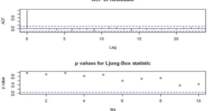
In this empirical study, the model development of the price series is accomplished using the fitting algorithm explained earlier which comprises of model identification, model estimation and model validation. The procedure is done with the assistance of software environment named R using the packages “forecast” and “tseries”. In Fig. 7, it is observable that the ACF residuals cut off from the first lag which deduce that the model and the data fit each other well [10]. Verification test introduced by Ljung et al. [23] is also shown in the result. Referring to the result obtained, the most fitted model will be selected to predict the testing data to assess the efficacy of the constructed model. This model development process describes the single forecasting model ARIMA approach.
Fig. 7. Model Validation Created using R Software Environment
For the proposed approach, each subseries will be treated as the input to develop their respective ARIMA model. The model development procedure will be similar to the one described previously. After the most fitted ARIMA model for each subseries has been successfully verified, the reconstruction of the decomposed subseries to acquire the original forecasted series is done using inverse DWT from Eq 3. The decomposition and reconstruction processes are done with the assistance of MATLAB software. Lastly, the calculation of MAE and RMSE for the single forecasting model ARIMA and the proposed approach are made using the forecast result with the testing data of the original price series to access their prediction accuracy.
D.Effectiveness Evaluation Result
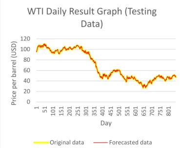
The MAE and RMSE results of testing data for the single forecasting model ARIMA and the proposed approach are exhibited in Table II below. Fig. 8 and Fig. 9 depict the graph of the forecasting results. From the graphs, it appears that both original and forecasted data can be matched completely, but actually there are differences in both data which are very small to be seen in current size. Smaller MAE and RMSE values indicate better forecasting accuracy of an approach. Referring to Table II, it is clear that the MAE and RMSE result of proposed approach is lesser than the results of single model ARIMA. In addition, all results in both datasets display that the proposed approach is better than single model ARIMA. For that reason, we can deduce that the proposed approach can give a superior and improved prediction outcome than the straightforward application of ARIMA model as anticipated.
Table II
MAEAND RMSERESULT OF TESTING DATA
Model WTI Brent
MAE RMSE MAE RMSE
Direct ARIMA 1.011699 1.318813 0.878396 1.161596
Wavelet-ARIMA
47 Fig. 8. WTI Daily Result Graph (Testing Data) using Proposed Approach
Fig. 9. Brent Daily Result Graph (Testing Data) using Proposed Approach
Besides comparing the models developed throughout the research, a comparison is also made between the models proposed by other literatures that utilized COSP series as the dataset. Table III depicts the result comparison between the previous works and the proposed approach. We only made comparison with existing works that utilized the same type of dataset as ours. Some data from existing studies are missing because they are unavailable in their works. From the result shown, it is observable that the proposed approach has managed to surpass all the previous existing models which concludes its effectiveness.
TABLE III
RESULT COMPARISON BETWEEN PROPOSED APPROACH WITH EXISTING
LITERATURES
Model WTI Brent
MAE RMSE MAE RMSE
WSVM [23] 0.5508 0.7667 - -
WMLR [24] 0.4834 0.6572 - -
WANN [1] - 0.7449 - 0.1851
EMD–FNN–ALNN
[4] - 0.273 - 0.225
EMD-ARIMA-ALNN
[4] - 0.975 - 0.872
GARCH [25] - 0.9518 - 1.8947
Proposed DWT –
ARIMA 0.1527 0.2275 0.1491 0.2005
IV.CONCLUSION
This empirical study presents a hybrid approach in crude oil spot prices forecasting. It combines wavelet transform as the data decomposition method and ARIMA as the forecasting method to enhance the forecasting accuracy. Wavelet transform is utilized to alter the price series behaviour from having volatile variance and outliers to become a set of subseries that exhibit stable variance and no outliers. Each subseries is then forecasted by applying ARIMA model and lastly combined back using inverse wavelet transform to achieve the forecast of the original series. Daily crude oil spot prices from Brent and WTI are chosen as the datasets in this empirical study. The experiment conducted compares the proposed approach with the single forecasting model ARIMA and other literatures that utilized COSP series in order to assess the efficacy of the proposed approach. The result of MAE and RMSE obtained has confirmed that the proposed approach can produce finer forecasting result than the other approaches included in the experiment.
ACKNOWLEDGMENT
The authors would like to express their deepest gratitude to Research Management Center (RMC) of Universiti Teknologi Malaysia (UTM), Ministry of Science, Technology and Innovation (MOSTI) and Ministry of Higher Education Malaysia (MOHE) for all their financial support under Grant Vot 4F875.
REFERENCES
[1] Shabri A. and R. Samsudin. (2014). Daily Crude Oil Price Forecasting Using Hybridizing Wavelet and Artificial Neural Network Model. Mathematical Problems in Engineering. [2] Azevedo V. G. and L. M. Campos. (2016). Combination of
Forecasts for the Price of Crude Oil on the Spot Market.
0 20 40 60 80 100 120
1 51
101 151 201 251 301 351 401 451 501 551 601 651 701 751 801
Price
p
er
b
ar
re
l (USD)
Day
WTI Daily Result Graph (Testing
Data)
Original data Forecasted data
0 20 40 60 80 100 120 140
1 52
103 154 205 256 307 358 409 460 511 562 613 664 715 766 817
Price
p
er
b
ar
re
l (U
SD)
Day
Brent Daily Result Graph (Testing
Data)
48
International Journal of Production Research, 54(17),
5219-5235.
[3] Nochai R. and T. Nochai. (2006). ARIMA Model for Forecasting Oil Palm Price. Proceedings of the 2nd IMT-GT Regional
Conference on Mathematics, Statistics and Applications, 13-15.
[4] Yu L., S. Wang, and K. K. Lai. (2008). Forecasting Crude Oil Price with an EMD-based Neural Network Ensemble Learning Paradigm. Energy Economics, 30(5), 2623-2635.
[5] Abosedra S. and H. Baghestani. (2004). On the Predictive Accuracy of Crude Oil Futures Prices. Energy Policy, 32(12), 1389-1393.
[6] Crowley P. M. (2007). A Guide to Wavelets for Economists.
Journal of Economic Surveys, 21(2), 207-267.
[7] Schlüter S. and C. Deuschle, Using Wavelets for Time Series
Forecasting: Does It Pay Off? 2010, IWQW Discussion Paper
Series.
[8] Kriechbaumer T., A. Angus, D. Parsons, and M. R. Casado. (2014). An Improved Wavelet–ARIMA Approach for Forecasting Metal Prices. Resources Policy, 39, 32-41. [9] Ediger V. Ş., S. Akar, and B. Uğurlu. (2006). Forecasting
production of fossil fuel sources in Turkey using a comparative regression and ARIMA model. Energy Policy, 34(18), 3836-3846.
[10] Yusof N. M., R. S. A. Rashid, and Z. Mohamed. (2010). Malaysia Crude Oil Production Estimation: An Application of ARIMA Model. International Conference on Science and Social
Research (CSSR), 1, 1255-1259. IEEE.
[11] Zhang J.-L., Y.-J. Zhang, and L. Zhang. (2015). A Novel Hybrid Method for Crude Oil Price Forecasting. Energy Economics, 49, 649-659.
[12] Cao S.-G., Y.-B. Liu, and Y.-P. Wang. (2008). A Forecasting and Forewarning Model for Methane Hazard in Working Face of Coal Mine based on LS-SVM. Journal of China University of
Mining and Technology, 18(2), 172-176.
[13] Conejo A. J., M. A. Plazas, R. Espinola, and A. B. Molina. (2005). Day-ahead Electricity Price Forecasting Using the Wavelet Transform and ARIMA Models. IEEE Transactions on
Power Systems, 20(2), 1035-1042.
[14] Nourani V., M. T. Alami, and M. H. Aminfar. (2009). A Combined Neural-wavelet Model for Prediction of Ligvanchai Watershed Precipitation. Engineering Applications of Artificial
Intelligence, 22(3), 466-472.
[15] Wang W.-c., K.-w. Chau, D.-m. Xu, and X.-Y. Chen. (2015). Improving Forecasting Accuracy of Annual Runoff Time Series using ARIMA based on EEMD Decomposition. Water
Resources Management, 29(8), 2655-2675.
[16] Shafie-Khah M., M. P. Moghaddam, and M. Sheikh-El-Eslami. (2011). Price Forecasting of Day-ahead Electricity Markets Using a Hybrid Forecast Method. Energy Conversion and
Management, 52(5), 2165-2169.
[17] Dooley G. and H. Lenihan. (2005). An Assessment of Time Series Methods in Metal Price Forecasting. Resources Policy, 30(3), 208-217.
[18] Hyndman R. J. and Y. Khandakar. (2007). Automatic Time
Series for Forecasting: The Forecast Package for R. Monash
University, Department of Econometrics and Business Statistics. [19] Nury A. H., K. Hasan, and M. J. B. Alam. (2017). Comparative Study of Wavelet-ARIMA and Wavelet-ANN Models for Temperature Time Series Data in Northeastern Bangladesh.
Journal of King Saud University-Science, 29(1), 47-61.
[20] Amjady N. and F. Keynia. (2008). Day Ahead Price Forecasting of Electricity Markets by a Mixed Data Model and Hybrid Forecast Method. International Journal of Electrical Power &
Energy Systems, 30(9), 533-546.
[21] Hu J. and J. Wang. (2015). Short-term Wind Speed Prediction Using Empirical Wavelet Transform and Gaussian Process Regression. Energy, 93, 1456-1466.
[22] Tan Z., J. Zhang, J. Wang, and J. Xu. (2010). Day-ahead Electricity Price Forecasting using Wavelet Transform Combined with ARIMA and GARCH Models. Applied Energy, 87(11), 3606-3610.