Duality in Nonlinear Fractional Programming Problem Using Fuzzy Programming and Genetic Algorithm

DOI : 10.14810/ijscmc.2015.4103 19

D

UALITY

I

N

N

ONLINEAR

F

RACTIONAL

P

ROGRAMMING

P

ROBLEM

U

SING

F

UZZY

P

ROGRAMMING

A

ND

G

ENETIC

A

LGORITHM

Ananya Chakraborty

Assistant Professor, Department of Mathematics, Vemana Institute of Technology, Kormangala 3rd Block, Bangalore-34. Karnataka, India

ABSTRACT

In this paper we have considered nonlinear fractional programming problem with multiple constraints. A pair of primal and dual for a special type of nonlinear fractional programming has been considered under fuzzy environment. Exponential membership function has been used to deal with the fuzziness. Duality results have been developed for the special type of nonlinear programming using exponential membership function. The method has been illustrated with numerical example. Genetic Algorithm as well as Fuzzy programming approach has been used to solve the problem.

KEYWORDS

Fuzzy Mathematical Programming, Nonlinear Fractional Programming, Exponential membership function, Decision Analysis, Genetic Algorithm.

1.

INTRODUCTION

Several factors in the real world imply the increase in use of nonlinear programming models. There are several classes of problems where nonlinear programming had had a great impact for example oil and petrochemical industries, nonlinear network problems and economic planning models. The area where nonlinear programming can be used in these several classes of problems is given in detail in (Ladson et al., 1980). The concept of fuzzy programming in decision making problem was first proposed by (Bellmann and Zadeh, 1970). Many authors have applied fuzzy programming approach in different area of linear programming (Zimmermann, 1978, Stancu-Minasian et al., 1978, Chakraborty and Gupta, 2002). In (Jimenez, 2005), author has considered a non linear programming problem with fuzzy constraints and the solution has been obtained by muti objective evolutionary Algorithms. An interactive cutting plane algorithm for fuzzy multi objective nonlinear programming problems has been presented in (Kanaya, 2010). In (Jameel, 2012), author has obtained accurate results for solving non linear programming using fuzzy environment by using properties of fuzzy set and fuzzy number with linear membership function.

20

minimization of cost/time, maximization of output/input, Non-Economic Applications. There are a number of management science problems which indirectly give rise to a fractional program; see e.g. (Schaible, 1981, 1983, 1995). A new method has been given by (Borza et al. 2012) for solving the linear fractional programming problems with interval coefficients in the objective function.

An algorithm has been developed by (Saad et al., 2011) for multi objective integer nonlinear fractional programming problem under fuzziness. In order to defuzzify the problem, he has developed the concept of α-level set of the fuzzy number is given and for obtaining an efficient solution to the problem (FMOINLFP), a linearization technique is presented to develop the solution algorithm. In the paper (Biswas and Bose, 2012) author presented a fuzzy programming procedure to solve nonlinear fractional programming problems in which the parameters involved in objective function are considered as fuzzy numbers.

The duality theory for nonlinear multiobjective optimization problems in the field of the optimization theory has intensively developed during the last decades. In (Rodder and Zimmermann, 1980), a generalization of maxmin and minmax problems in a fuzzy environment is presented and thereby a pair of fuzzy dual linear programming problems is constructed. An economic interpretation of this duality in terms of market and industry is also discussed in that paper. In (Bector and Chandra, 2002), a pair of linear programming primal-dual problem is introduced under fuzzy environment and appropriate results were proved to establish the duality relationship between them. In (Liu, 1995) a constructive approach has been proposed to duality for fuzzy multiple criteria and multiple constraint level linear programming problems. (Biswas and Bose, 2012) gives a parametric approach for the duality in fuzzy multi criteria and multi constraint level linear programming problem. In (Gupta and Mehlawat , 2009), a study of a pair of fuzzy primal–dual linear programming problems has been presented and calculated duality results using an aspiration level approach using exponential membership function, while a discussion of fuzzy primal dual linear programming problem with fuzzy coefficients has been presented in (Bector and Chandra, 2002; Liu, 1995). In (Bector and Chandra, 2002), a pair of linear programming primal-dual problem is introduced under fuzzy environment and appropriate results were proved to establish the duality relationship between them. Also in (Chakraborty et al. 2014), author has presented a pair of linear primal – dual programming using linear and exponential membership function using fuzzy programming approach and genetic algorithm approach.

In this paper we have extended the work done by (Gupta and Mehlawat , 2009) in which he has solved duality in convex fractional programming using linear membership function. We have taken the same kind of problem and proved the duality theorems considering exponential membership function for fuzzified objective function and constraints and then solved using LINGO and Genetic Algorithm also and the results have been analysed.

The paper has been organized as follows: In section 2, the nonlinear fractional programming problem and its dual has been defined. The fuzzified and the crisp formulation have been defined for the primal and dual. In section 3, the necessary duality results have been developed. The numerical example defined in (Gupta and Mehlawat , 2009) has been illustrated in section 4. Finally, analysis of the solution and concluding remarks has been presented in section 5.

2.

NON LINEAR FRACTIONAL PROGRAMMING PROBLEM

21

2

( ) Max ( )

t

t c x f x

d x

=

Subject to

Ax

≤

b

0

x

≥

(1)

The dual form of the above problem can be written as Min g u v( , )=b ut

Subject to _{A u}t _+dv2_≥2_cv , 0 u v≥

(2)

Where A is m x n matrix, x, c, b are column vectors with n components and b is a column vector of m components.

2.1 Fuzzified Non Linear Fractional Programming Problem

Fuzzified form of nonlinear fractional programming problem can be defined as

Find x∈Rn

Subject to

2 ~ 0

( ) ( )

t

t c x

f x Z

d x

= ≥

~

Ax b≤

x

≥

0

(3)

Where Z0 is the aspiration level of the objective function of the primal problem. “ ~

≤” and “

~

≥” denotes the flexibility of the objective function and the multi constraints.

Fuzzified form of the dual of the problem can be defined as

Find u∈Rm

Subject to

~ 0

g(u,v)=u b wt ≤

~ 2

2 t

A u+dv ≥ cv

u v, ≥0 (4) Where w0 is the aspiration level of the objective function of the dual problem.

2.2 Crisp Formulations using Exponential Membership Function

22

representation. Furthermore, if the membership function is interpreted as the fuzzy utility of the decision maker, used for describing levels of indifference, preference towards uncertainty, then a nonlinear membership function provides a better representation than a linear membership function. Moreover, unlike linear membership function, for nonlinear membership functions the marginal rate of increase (or decrease) of membership values as a function of model parameters is not constant- a technique that reflects reality better than the linear case (Gupta and Mehlawat , 2009).

Let us consider the following form of exponential membership function (Gupta and Mehlawat , 2009; Chakraborty et al. 2014) for the fuzzy nonlinear fractional programming problem respectively.

(

)

(

)

2 0 2 0 ( ) / 2 0 0 c 1 c ( ) z

1-0 t t t t c x z p d x t t x if z d x x e e

x if p z

e d x

i α α α

µ

     − _ − _−  −      − ≥ −

= − < <

(

)

2 0

c t_tx

f z p

d x                    ≤ −        {( ) / } 1 ( ) 1-0

j j j j j

j

j j

b A x q

j j j j j

j j j

if A x b

e e

x if b A x b q

e

if A x b q

α α α

µ

− − − − − ≤   − 

= < < +

  _{≥ +}        

j=1, 2,…….m

(5)

Where

α

and

α

_j are user defined parameters which determine the shape of the membership function. p and qj (j = 1, 2, …..m) are subjectively chosen constant of admissible violations such

that pis associated with nonlinear fractional objective function and q s_j' are associated with m linear constraints of the problem.

Therefore using exponential membership function the crisp formulation of the problem can be given by

Max ߣ

Subject to

( )2 0 / 1-t t c x z p d x e e e α α α

λ

   _{ }  − _ − _−     −   − − ≤ {( ) / }

1-j j j j j

j

b A x q

e

e

e

α α α

λ

− − − − −

−

≤

j=1, 2,…m

23

or Max ߣ

Subject to

(

)

2

0

log{ (1 ) } c xt_t

p e e z

d x

α α

λ

− −

α

 

− + ≤ _ − _

 

log{ (1 j) j} ( )

j j j j

q

λ

−e−α +e−α ≤

α

b −A x , j =1, 2,…m

ߣ_{≤ 1,} ߣ_{≥ 0, x≥ 0. (7)}

The exponential membership function for the dual problem objective function and nonlinear constraints are given by

0

0

{( ( , )) / }

0 0

0

1 if ( , ) ( ) if ( , )<

1-0 if ( , ) w g u v r

g u v w

e e

w w g u v w r

e

g u v w r

β β

β

µ

− − − −

−

 _≤



−

= < +

≥ +

 

 



 

 

 

2

t 2

{( 2 ) / }

t 2

t

1 if A 2

( ) if 2 <A 2

1-0 if A

t

j j j j j

j

j j

A u d v c v s

j j j j j

u d v c v

e e

w c v s u d v c v

e

u

β β

β

µ

− + − − −

−

+ ≥

−

= − + <

2

2

j j j

d v c v s

 

 

 

 

 

 

 _{+ ≤ −} 

 

 _{j = 1, 2,…,n}

(8)

Where

β

and

β

_j's are user defined parameters which determine the shape of the membership function. r and sj (j = 1, 2, ……., n) are subjectively chosen constant of admissible violations

such that r is associated with objective function and s s_j' are associated with n linear constraints of the dual problem.

Min (-η)

Subject to

{

₍ 0 _{( , )) /}

}

1-w g u v r

e

e

e

β _β

β

η

− − − ₋

−

−

≤

2

{( 2 ) / }

1-t

j j j j j

j

A u d v c v s

e

e

e

β β

β

η

− + − − −

−

−

≤

j=1, 2,…n

η≤ 1, η≥ 0, u,v≥ 0. (9)

or Min (-η)

Subject to rlog{ (1

η

e−β) e−β}

β

(

w0 g u v( , )

)

24

2

log{ (1 j) j} ( t 2 )

j j j j j

s

η

−e−β +e−β ≤

β

A u+d v − c v , j=1, 2,…n

η≤ 1, η≥ 0, u,v ≥ 0. (10)

3.

THEOREMS ON DUALITY

We shall prove some duality theorems. In the theorems, Q= (q1, q2, ……,qm), S= (s1, s2, ……., sn )

are column vectors

Theorem 3.1 (Modified fuzzy weak duality theorem): Let (x, ߣ_{) be the feasible solution of crisp}

primal problem (7) and (u, v,

η

) be feasible solution of crisp dual problem (10). Then

2 ~

1 1

log{ (1 i) i} log{ (1 j) j} ( t )

m n

t t t

t

i i j j

e e e e c x

u Q S x u b

d x β β α α

λ

η

α

β

− − − − = = − + − + + ≤ −

∑

∑

Proof: Since (x, ߣ_{) be the feasible solution of crisp primal problem (7) and (w,}

_η

_{) be feasible}

solution of crisp dual problem (10), then

log{ (1 i) i} ( )

i i i i

q

λ

e−α e−α

α

b A x

− + ≤ − , i=1, 2,…m

2

log{ (1 j) j} ( t 2 )

j j j j j

s

η

−e−β +e−β ≤

β

A u+d v − c v , j=1, 2,…n

Or

1

log{ (1 i) i} m

i i

e e

Q b Ax

α α

λ

α

− − = − + ≤ −

∑

(11)

2

1

log{ (1

)

}

2

j j n t j j

e

e

S

A u

dv

cv

β β

η

β

− − =

−

+

≤

+

−

∑

(12)

Multiplying the equation (11) by transpose of u and taking transpose of equation (12) and multiplying equation by x, we have

1

log{ (1 i) i} m

t t t

i i

e e

u Q u b u Ax

α α

λ

α

− − = − + ≤ −

∑

2 1

log{ (1

)

}

2

j j

n

t t t t t t

j j

e

e

S x

u Ax v d x

v c x

β β

η

β

− − =

−

+

≤

+

−

∑

Adding the above two inequalities, we have

2

1 1

log{ (1

)

}

log{ (1

)

}

2

j j

i i

m n

t t t t t t t

i i j j

e

e

e

e

u Q

S x

u b v d x

v c x

β β α α

λ

η

α

β

− − − − = =

−

+

−

+

+

≤

+

−

∑

∑

Or 1

2

1 2

2 ₂

1 1

log{ (1 ) } log{ (1 ) } ( ) ( )

( )

( )

j j

i i t t

m n

t t t t t

t t

i i j j

e e e e c x c x

u Q S x u b d x v

25 1 2 1 2 2 2 1 1

log{ (1 ) } log{ (1 ) } ( ) ( )

( )

( )

j j

i i t t

m n

t t t t

t t

i i j j

e e e e c x c x

u Q S x u b d x v

d x d x

β β α α λ η α β − − − − = =     − + − + + ≤ −  + −     

∑

∑

2 ~ 1 1

log{ (1 i) i} log{ (1 j) j} ( t )

m n

t t t

t

i i j j

e e e e c x

u Q S x u b

d x β β α α

λ

η

α

β

− − − − = =   − + − + + ≤ −   

∑

∑

Remark: When ߣ_=1,

_η

_{=1 in the above inequality we get the objective function of primal}

problem is imprecisely less than the objective function of the dual

2 ~ ₍ t ₎

t t c x u b d x   ≤  

 which can be defined as the standard fuzzified weak duality theorem in a multi objective linear programming problem.

Theorem 3.2:Let(

^ ^

,

x

λ

) be feasible solution of crisp primal problem (7) and (

^ ^

,

w

η

) be feasible solution of crisp dual problem (10) such that

(i) ^ ^ ^ 2 ^ _^ ^ ^ 1 1

log{ (1 i) i} log{ (1 j) j} ( t )

m n

T T t

t

i i j j

e e e e c x

w Q S x u b

d x β β α α

λ

η

α

β

− − − − = = − + − + + = −

∑

∑

(ii) ^ ^ ^ 2 ^ 0 0 ^

log{ (1 ) } log{ (1 ) } ( )

( )

t

t

t

e e e e c x

p r u b w z

d x

α α β β

λ

η

α

β

− − − −   − + − + _{ } + = − + −    

(iii) The aspiration levels z0and w0 satisfy (z₀−w₀)≤0

Then (

^ ^

,

x

λ

) is optimal solution of primal problem and (

^ ^

,

w

η

) be optimal solution of dual problem.

Proof: Let (x, ߣ_{) be feasible solution of crisp primal problem (7) and (w,}

_η

_{) be feasible solution}

of crisp dual problem (10). Then from Theorem 3 we have,

( )

2 ~

1 1

log{ (1 ) } log{ (1 ) }

0

j j

i i t

m n

t t t

t

i i j j

c x

e e e e

u Q S x u b

d x β β α α λ η α β − − − − = =   − + − + _{ } + − − ≤    

∑

∑

(13)

From condition (i) and Equation (13) we have

( )

2

lo g { (1 ) } lo g { (1 ) }

1 1

t c x

m _e i _e i _t n _e j _e j _{t t}

u Q S x u b

t

i j d x

i j

α α β β

λ η α β     − − − − − + − + _{ } ∑ + ∑ − −   = = _{ }   2 ^ ^ ^ ^ ^ ~ ^ ^ 1 1

log{ (1 i) i} log{ (1 j) j}

t

m n

t t t

t

i i j j

c x

e e e e

u Q S x u b

26

Thus,

^ ^ ^ ^

( , , , )x

λ

w

η

is optimal to the problem whose maximum objective value is 0.

Max

( )

2

lo g { (1 ) } lo g { (1 ) }

1 1

t c x

m _e i _e i _t n _e j _e j _{t t}

u Q S x u b

t

i j d x

i j

α α β β

λ η α β     − − − − − + − + _{ } ∑ + ∑ − −   = = _{ }   Subject to

( )

2 0

log{ (1 ) }

t

t c x

p e e Z

d x

α α

λ

− −

α

 

 

− + ≤ −

 

 

log{ (1 i) i} ( )

i i i i

q

λ

e−α e−α

α

b A x

− + ≤ −

(i = 1, 2, ……, m)

0

log{ (1 ) } ( t )

r

η

e−β e−β

β

w u b

− + ≤ −

2

log{ (1 j) j} ( t 2 )

j j j j j

s

η

−e−β +e−β ≤

β

A u+d v − c v

(j = 1, 2, …….., n )

ߣ_{≤ 1,} ߣ_{≥ 0, x≥ 0,}

_η

_{≤1, ,u v≥0,}

_η

_≥0.

Adding condition (i) and (ii), we have

( )

2

lo g { (1 ) } lo g { (1 ) }

1 1

t c x

m _e i _e i _t n _e j _e j _{t t}

u Q S x u b

t

i j d x

i j

α α β β

λ η α β     − − − − − + − + _{ } ∑ + ∑ − −   = = _{ }   + ^ ^ ^ 2 ^ 0 0 ^

log{ (1 ) } log{ (1 ) } ( )

( ) 0

t

t t

e e e e c x

p r u b w z

d x

α α β β

λ

η

α

β

− − − −   − + − + _{ } + − − − − =     Or

lo g { (1 ) } lo g { (1 ) }

1 1

m _e i _e i _t n _e j _e j _t

u Q S x

i j

i j

α α β β

λ η α β − − − − − + − + ∑ + ∑ = = + ^ ^ 0 0

log{ (1 ) } log{ (1 ) }

( ) 0

e e e e

p r z w

α α β β

λ

η

α

β

− − − −

− + − +

+ + − =

Each term in the above sum is non positive as

^ ^

, 1.

λ η

≤

Therefore,

^

^

1

log{ (1

i

)

i

}

m t i i

e

e

u Q

α α

λ

α

− − =

−

+

∑

= 0

^

x t ^

1

log{ (1 ) }

0 j j n t j j e e S x β β

η

β

− − = − + =

∑

^

log{ (1

)

}

27

^

log{ (1 ) }

0

e e

r

β β

η

β

− −

− +

=

z₀−w₀=0

Since log{ (1 e ) e }p 0

α α

λ

α

− −

− +

≤ and

log{ (1

e

)

e

}

r

0,

β β

η

β

− −

−

+

≤

because

^ ^

, 1

λ η

≤ , we get

^

log{ (1

e

)

e

}

log{ (1

e

)

e

}

p

p

α α α α

λ

λ

α

α

− − − −

−

+

−

+

≤

^

log{ (1 e ) e } log{ (1 e ) e }

r r

β β β β

η

η

β

β

− − − −

− + − +

≤

or

^

λ

≤

λ

and

^

η η

≤

Thus, (

^ ^

,

x

λ

) is optimal solution of (7) and (

^ ^

,

w

η

) be optimal solution of (10).

4.

NUMERICAL EXAMPLE

Let us consider the same numerical example which is defined in [20]. The primal dual nonlinear fractional programming problem can be defined as

Min

2

1 2

1 2

(2 )

( )

2 x x f x

x x

+ =

+

Subject to

2

x

₁

+

x

₂

≥

6

x

₁

+

3

x

₂

≥

8

x x

₁

,

₂

≥

0

Max

g u v

( , )

=

6

u

₁

+

8

u

₂

Subject to 2u₁+u₂+v2−4v≤0

u₁+3u₂+2v2−2v≤0

u u v

₁

,

₂

,

≥

0

The fuzzified nonlinear fractional programming problem can be written as:

Find x∈Rn

Min

Subject to

2 ~

1 2

1 2

(2 )

( ) 1

2 x x f x

x x

+

= ≤

+

~

1 2

28

~

1 3 2 8

x + x ≥

x x

₁

,

₂

≥

0

(14) Max

~

1 2

( , ) 6 8 1 g u v = u + u ≥

Subject to

~ 2

1 2

2u +u +v −4v≤0

~ 2

1 3 2 2 2 0

u + u + v − v≤

u u v

₁

,

₂

,

≥

0

(15)

Let us take

p

=

2,

q

₁

=

1,

q

₂

=

1,

α

=

2,

α

₁

=

2,

α

₂

=

1

for primal problem. Using exponential membership function, the crisp model of (14) can be written as:

Min

−

λ

Subject to 4x₁2+x2₂+4x x_{1 2}≥(x₁+2 ) log(0.865x₂

λ

+0.1353)

4

x

₁

+

2

x

₂

−

12

≥

log(0.865

λ

+

0.1353)

x

₁

+

3

x

₂

− ≥

8

log(0.865

λ

+

0.1353)

ߣ_{≤ 1,} ߣ_{≥ 0}

x x

₁

,

₂

≥

0

. (16)

Let us take

r

=

1,

s

₁

=

1,

s

₂

=

1,

β

=

2,

β

₁

=

2,

β

₂

=

1

for dual problem (15). Using exponential membership function, the crisp model can be written as:

Max

η

Subject to

log(0.865

η

+

0.1353) 12

≤

u

₁

+

16

u

₂

−

2

2

1 2

log(0.865

η

+0.1353)≤ −4u −2u −2v +8v

2

1 2

log(0.865

η

+0.1353)≤ −u −3u −2v +2v

0≤

η

≤1,

u u v

₁

,

₂

,

≥

0

. (17)

5.

SOLUTION AND ANALYSIS

Using LINGO software, the solution of the primal problem (16) is given by

Local optimal solution found.

29

Total constraints: 5

Nonlinear constraints: 3

Total nonzeros: 11

Nonlinear nonzeros: 5

Variable Value LAMBDA 1.000000 X1 1.234568 X2 0.1000000E+08 Minimum value of objective function is -1. The solution of the dual problem (17) is given by Local optimal solution found. Objective value: 1.000000 Infeasibilities: 0.000000 Extended solver steps: 5

Total solver iterations: 37

Model Class: NLP Total variables: 4

Nonlinear variables: 2

Integer variables: 0

Total constraints: 5

Nonlinear constraints: 3

Total nonzeros: 13

Nonlinear nonzeros: 5 Variable Value

ETA 1.000000 U1 0.1037300 U2 0.4665636E-01 V 0.1359680

Maximum value of the objective function is 1.

Genetic Algorithm gives global optimal solution. The NSGA used here is a real parameter GA that works directly with the parameter values. NSGA (Nondominated Sorting Genetic Algorithm) uses nitching, as well as nondominated sorting of the solutions in every generation to ensure that the “good solutions get preference in selection for procreation”. The non-dominated sorting GA uses a ranking selection method to emphasize good solutions and then a nitche building procedure to maintain a stable sub population of good solutions. Since multi objective GAs can find multiple pareto optimal solutions in one single run, the proposed technique is capable of finding multiple solutions to the problems.

The parameters used to solve the problem (16) in Genetic Algorithm are as follows:

30

Objective function # 1 : Minimize

CROSSOVER TYPE : Binary GA (Single-pt) STRATEGY : 1 cross - site with swapping Population size : 100

Total no. of generations : 100 Cross over probability : 0.9000 Mutation probability : 0.1000 String length : 60 Number of variables Binary : 3 Integer : 0 Enumerated : 0 Continuous : 0 TOTAL : 3

Epsilon for closeness : 0 Sigma-share value : 0.2320

Sharing Strategy : sharing on Parameter Space

Lower and Upper bounds : 0.0000 <= ߣ _{<= 1.0000}

0.0000 <= x1 <= 2.0000

0.0000 <= x2 <= 2.0000

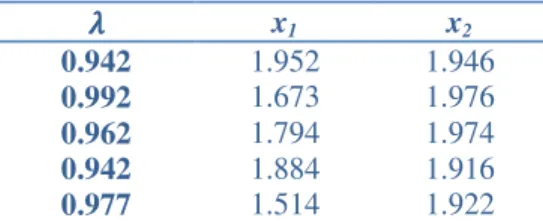
Table 1 gives a set of solution of problem (16).

Table 1: Primal Solution

ߣ ߣ ߣ

ߣ _{x1 x2}

0.942 1.952 1.946

0.992 1.673 1.976

0.962 1.794 1.974

0.942 1.884 1.916

0.977 1.514 1.922

The parameters used to solve the problem (17) in Genetic Algorithm are as follows: Number of objective functions : 1

Objective function # 1 : Maximize

CROSSOVER TYPE : Binary GA (Single-pt)

STRATEGY : 1 cross - site with swapping Population size : 100

31

Integer : 0 Enumerated : 0 Continuous : 0 TOTAL : 4

Epsilon for closeness : 0 Sigma-share value : 0.2810

Sharing Strategy : sharing on Parameter Space Lower and Upper bounds :

0.0000 <= u1 <= 2.0000

0.0000 <= u2 <= 2.0000

0.0000 <= v <= 2.0000 0.0000 <= η <= 1.0000

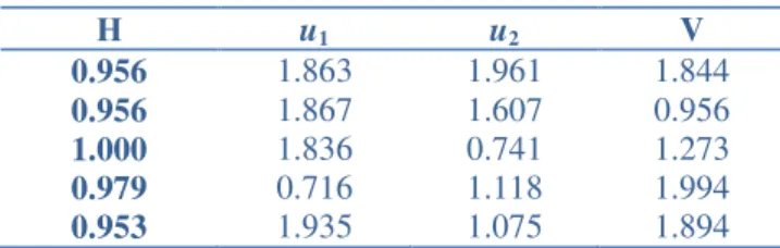
Using Genetic algorithm, a set of solutions of dual problem (17) is given in the form of table in Table 2.

Table 2: Dual Solution

Η u1 u2 V

0.956 1.863 1.961 1.844

0.956 1.867 1.607 0.956

1.000 1.836 0.741 1.273

0.979 0.716 1.118 1.994

0.953 1.935 1.075 1.894

32

6.

CONCLUSIONS

In this paper, an approach has been presented for a specific kind of fuzzy nonlinear fractional programming problem by constructing a pair of fuzzy non linear fractional primal and dual problems. Crisp form of the above primal and dual problems has been obtained by using exponential membership function. Duality results have been established to prove the duality relationship between above primal and dual problem and are illustrated by an example. The duality results fully satisfy the aspiration levels or the tolerance levels of the objective functions and the system constraints made by the decision maker. The difference between the achieved level and the allowable limit of the satisfying solutions of the decision maker is very less. The numerical example has also been solved by Genetic Algorithm Approach. Genetic Algorithm gives multiple pareto optimal solution. The decision maker can choose any optimal solution according to the convenience. The results of the present paper encourage us to apply duality results in variety number of fields of optimization problem.

REFERENCES

[1] Bellman, R. E., Zadeh, L. A., (1970) Decision Making in a Fuzzy Environment, Management Science, 17, 141-164.

[2] Bector, C. R. and Chandra, S., (2002) On duality in linear programming under fuzzy environment, Fuzzy Sets and Systems, 125, 317-325.

[3] Biswas, A. and Bose, K., (2012), Application of Fuzzy Programming Method for Solving Nonlinear Fractional Programming Problems with Fuzzy Parameters, Mathematical Modelling and Scientific Computation Communications in Computer and Information Science 283 104-113.

[4] Borza, M., Rambely, A. S. and Saraj, M., (2012) Solving linear fractional programming problems with interval coefficients in the objective function. A New Approach, Applied Mathematical Sciences, 6, 69, 3443 – 3452.

[5] Chakraborty, M., Gupta, S., (2002) Fuzzy Mathematical Programming for Multi-objective Linear Fractional Programming Problem, Fuzzy Sets and Systems, 125, 335-342.

0.942

0.992

0.962

0.942

0.977

0.956 0.956

1

0.979

0.953

0.91 0.92 0.93 0.94 0.95 0.96 0.97 0.98 0.99 1 1.01

1 2 3 4 5

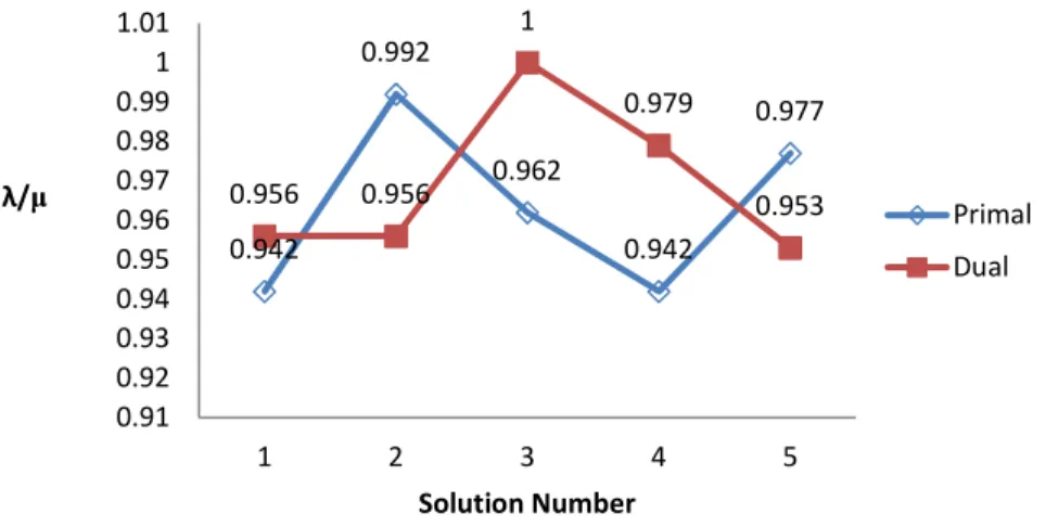
λ/µ

Solution Number

Figure 1: Primal and Dual objective function of different solution using GA

Primal

33 [6] Chakraborty, A., Tiwari, S. P., Chattopadhyay, A. and Chatterjee, K. (2014), Duality in Fuzzy Multi

objective linear programming with multi constraint, International Journal of Mathematics in Operations Research, Vol. 6, No. 3, pp. 297-315.

[7] Gupta, P. and Mehlawat, M. K., (2009) Duality for a convex fractional programming under fuzzy environment, International Journal of Optimization: Theory Methods and Applications, 1, 3, 291-301. [8] Gupta, P. and Mehlawat, M. K., (2009), Bector- Chandra type duality in fuzzy linear programming

with exponential membership functions, Fuzzy Sets and Systems, 160, 22, 3290-3308.

[9] Jameel, A. F., Sadhegi, A., (2012), Solving Nonlinear Programming Problem in Fuzzy Environment, Int. J. Contemp. Math. Sciences 7, 4, 159 – 170.

[10] Jimenez, F., Sanchez, G., Cadenas, J. M., Gomez-Skarmeta, A. F., Verdegay, J. L., (2005), Computational Intelligence, Theory and Applications, Advances in Soft Computing, 33, 713-722. [11] Kanaya, Z. A. (2010) An Interactive Method for Fuzzy Multiobjective Nonlinear Programming

Problems, JKAU: Sci. 22 1 103-112; DOI: 10.4197 / Sci. 22-1.8.

[12] Lasdon, L. S, Waren, A. D., (1980), Feature Article: Survey of Nonlinear Programming Applications, Operations Research 28(5): 1029-1073.

[13] Liu, Y. J., Shi, Y. and Liu, Y. H. (1995) Duality of fuzzy MC2 linear programming: a constructive approach, J. Math. Anal. Appl., 194, 389-413.

[14] Rodder, W. and Zimmermann, H. J. (1980), Duality in fuzzy linear programming. In: (A. V. Fiacco, K. O. Kortane K Eds.). External methods and System Analysis. Berlin, New York, 415-429.

[15] Saad, O. M., M. S. Biltagy and T. B. Farag, An algorithm for Multi objective Integer nonlinear fractional programming problem under fuzziness, Gen. Math. Notes, 2 1 (2011) 1-17.

[16] Schaible, S., (1981) Fractional programming: applications and algorithms, European Journal of Operational Research, 7, 2, 111-120.

[17] Schaible, S., (1995), Fractional programming, in R. Horst and P.M. Pardalos (eds.), Handbook of Global Optimization, Kluwer Academic Publishers, Dordrecht-Boston-London, 495-608.

[18] Schaible, S. and Ibaraki, T., (1983), Fractional programming, European Journal of Operational Research 12, 3, 325-338.

[19] Stancu-Minasian, I. M., Pop, B., (1978) On a Fuzzy Set Approach to Solving Multiple Objective Linear Fractional Programming Problem, Fuzzy Sets and Systems, 134, 397-405.

[20] Zimmermann, H. J., (1978) Fuzzy programming and linear programming with several objective functions, Fuzzy Sets and Systems, 1, 45-55.

Authors

Ananya Chakraborty is Assistant Professor in the Department of Mathematics of Vemana Institute of Technology, Bangalore, India. She has done her Ph.D from Indian School of Mines, Dhanbad, Jharkhand, India. She is having almost 10 years of research experience. She has published many papers in national/ international journals. She has presented many papers

in different conferences. Her current research interest includes Fuzzy programming, Operations Research. She is also a member of International association of computer science and information technology