Machine Cell Formation Based on a New Similarity Coefficient

(1)

Vol. 1, No. 4, pp 318-344 Winter 2008

Machine Cell Formation Based on a New Similarity Coefficient

Ibrahim H. Garbie1*, Hamid R. Parsaei2 and Herman R. Leep3

1

Department of Mechanical Engineering, Helwan University, Helwan, Cairo, 11792, EGYPT. [email protected]

2

Department of Industrial Engineering, University of Houston, Houston, TX, 77204, USA.

3

Department of Industrial Engineering, University of Louisville, Louisville, KY, 40292, USA. ABSTRACT

One of the designs of cellular manufacturing systems (CMS) requires that a machine population be partitioned into machine cells. Numerous methods are available for clustering machines into machine cells. One method involves using a similarity coefficient. Similarity coefficients between machines are not absolute, and they still need more attention from researchers. Although there are a number of similarity coefficients in the literature, they do not always incorporate the important properties of a similarity coefficient satisfactorily. These important properties include alternative routings, processing time, machine capacity (reliability), machine capability (flexibility), production volume, product demand, and the number of operations done on a machine. The objectives of this paper are to present a review of the literature on similarity coefficients between machines in CMS, to propose a new similarity coefficient between machines incorporating all these important properties of similarity, and to propose a machine cell heuristic approach to group machines into machine cells. An example problem is included and demonstrated in this paper.

Keywords: Cellular manufacturing, Similarity coefficients, Machine cells 1. INTRODUCTION

Cluster analysis has been used to study similarity measures and coefficients. Similarity coefficient approaches, which were used in grouping machines into cells, have received considerable attention in the literature. The machine–part incidence matrix is the input for most problems involving machine clustering. The machine-part incidence matrix is a zero-one matrix, [A], where element

ij

a =1 indicates that part j is processed on machine i. Although several methods are available in the

literature to cluster machines into machine cells, similarity coefficient approaches represent a well-known methodology in grouping machines, and they are more flexible in incorporating various types of manufacturing data. A wide range of similarity coefficient measures between machines will be explained in the review.

This paper is structured as follows. Section 2 reviews most of the papers published in the area of similarity coefficients between machines. Section 3 presents the proposed similarity coefficient between two machines. The heuristic approach which was used to group machines into machine

*

(2)

cells is presented in Section 4. Section 5 describes the analytical example. Section 6 presents the conclusion.

2. LITERATURE REVIEW

This section presents a comprehensive review of the research work of similarity coefficients between machines are related to the problem of finding similarity between two machines.

Viswanathan (1996) proposed similarity coefficient between two machines for P-median formulation as follows:

∑

=

n k

jk ik

ij

a

S

1

,

)

(

δ

(1)

2 )

(

a

_ik_,

a

_jk

=

δ

, if element

a

_ik

=

a

_jk

=

1

1 )

(

a

_ik_,

a

_jk

=

−

δ

, if

a

ik

≠

a

jk

0 )

(

a

ik,

a

jk

=

δ

, otherwise

k = subscript of part, k = 1,…, n (parts)

Viswanathan (1996) used positive and negative values, revealing the extent of similarity as well as dissimilarity. The machines were first clustered by solving for the P-median, and then the parts were assigned to the cells so as to minimize the number of voids inside the cells and the number of ones outside the cells. In this case, he ensured that each cell has at least two parts and two machines. Jaccard’s similarity coefficient equation (McAuley, 1972) is defined as follows:

ij j

i

ij ij

N N

N N S

− +

= (2)

ij

S

similarity coefficient between machines i and j.

ij

N

number of common parts processed by both machines i and j.

i

N

number of parts processed by machine i only.

j

N

number of parts processed by machine j only.

Aljaber et al. (1997) modified Jaccard’s similarity measure (McAuley, 1972) between two machines by subtracting it from its upper bound of 1, and it can be defined as follows:

ij j i

ij ij

N N N

N S

− + −

(3)

Won and Kim (1997) modified Jaccard’s similarity coefficient between two machines to produce a generalized similarity coefficient including alternative routings (process plans) of parts. They

defined the generalized machine similarity coefficient between two machines i and j as follows:

ij j i

ij ij

gsc

δ δ δ

δ

− +

= (4)

ij

gsc

generalized similarity coefficient between machines i and j.

ij

δ

number of common parts with multiple process routings processed by both machines i

and j. i

δ

number of parts with multiple process routing processed by machine i only.

j

δ

number of parts with multiple process routing processed by machine i only.

∑

=

= n k

i i k

1

) , (

α

δ ,

∑

=

= n k

j j k

1

) , (

α δ

1 )

,

(

i

k

=

α

if

a

_ikr

=

1

for some

r

∈

R

_k

0 )

,

(

i

k

=

α

otherwise

1 )

,

(

j

k

=

α

if

a

_jkr

=

1

for some

r

∈

R

_k

0 )

,

(

j

k

=

α

otherwise

k = 1,…, n (parts)

k

R

set of process routings of part k

∑

=

= n

k

ij Bi jk

1

) , , (

δ

1 )

,

(

i

j

k

=

B

if

a

_ikr

=

a

_jkr for some

r

∈

R

_k,

i

≠

j

0 )

,

(

i

j

k

=

B

otherwise

Yin and Yasuda (2002) modified the similarity coefficient of Won and Kim (1997) by incorporating

a sequence ratio (SR_ij ) and machine load ratio (MLRij) into equation (4). Then, they defined a new

similarity as follows:

ij ij ij j i

ij

ij SR MLR

gsc * *

δ

− +

= (5)

ij

SR

sequence ratio =

ij ij

D X

ij

MLR machine load ratio =

ij ij

E Y

ij

X

number of actual movements of parts between machines i and j

ij

D

number of possible movements of parts between machines i and j

ij

Y

minimum production volume factor between machine i and j

ij

(4)

Yin and Yasuda (2002) suggested also another similarity coefficient between machine cells (P and

Q) as follows:

Q P

P

i j Q

ij PQ

NM

gsc

S

×

=

∑∑

∈ ∈

(6)

P

NM

number of machines in cell P.

Q

NM number of machines in cell Q.

Won (2000) suggested two similarity coefficients between two machines for the P-median of machine cell formation under the assumption that each part may be processed by alternative process

plans. The first coefficient reflects the extent of similarity between machines i and j, and it is

defined as follows:

∑

=

= n

k

ij i j k

S 1 1

) , , (

α (7)

if

i

≠

j

, i , j = 1,…, m

0

1

=

ij

S

otherwise

1 )

,

(

i

j

k

=

α

, if

a

ikr

=

a

jkr

=

1

for some

r

∈

R

k k = 1,…, n

α

(

i

,

j

,

k

)

=

0

, otherwise

The second coefficient reflects the extent of similarity as well as dissimilarity between two machines as follows:

∑

=

= n

k

ij i j k

S

1 2

) , , (

β (8)

if

i

≠

j

, i, j = 1,…, m 0

2 =

ij

S otherwise

n

k

j

i

,

)

=

(

β

if

a

_ikr

=

a

_jkr

=

1

for some

r

∈

R

_k

1 )

,

(

i

j

k

=

−

β

if

a

ikr

≠

a

jkr for all

r

∈

R

k

0 )

,

(

i

j

k

=

β

if otherwise

n number of parts, m = number of machines

Nair and Narendran (1998) defined a new similarity coefficient and incorporated production

sequence and product volume to form cells. Then, the similarity coefficient between machines i and

j can be described as the ratio of the sum of the moves common to machines i and j, and the sum of

the total number of moves to and from machines i and j as follows:

j i

j i ij

t t

C C S

+ + =

) 0

(5)

∑ ∑

= =

=

n

k n

p

kip k i

iki

t

w

t

1 1

,

∑∑

= =

=

n

k n

p kjp k j

kj

t

w

t

1 1

,

∑∑

= =

= n

k n

p kip k i

ki c w C

1 1

,

∑∑

= =

= n

k n

p

kjp k j

kj c w C

1 1

i

t

accounts for the total number of moves to and from machine i by components which

visit it. j

t

accounts for the total number of moves to and from machine j by components which

visit it. i

C

takes into account the total number of moves to and from machine i made by all

components which visit machines i and j.

j

C

takes into account the total number of moves to and from machine j made by all

components which visit machines i and j.

0 =

kip

t

if

b

_kip

=

0

1 =

kip

t

if

b

kip

=

1

or

r

k

2 =

kip

t

otherwise

0 =

kjp

t

if

b

kjp

=

0

1 =

kjp

t

if

b

_kjp

=

1

or

r

_k

2 =

kjp

t

otherwise

0 =

kip

c

if

b

_kip

=

0

or

b

_kjp

=

0

1 =

kip

c

if

b

kip

=

1

or

b

kjp

=

1

or

r

k

2 =

kip

c

otherwise

0 =

kjp

c

if

b

kip

=

0

or

b

kjp

=

0

1 =

kjp

c

if

b

_kip

=

1

or

b

_kjp

=

1

or

r

_k

2 =

kjp

c

otherwise

k

w

weight of component k

k

r

maximum number of operations for component k

kip

b

operation sequence number if the kth (1≤k ≤n) component visits the ith (1≤i≤m)

machine for the pth (

1 ≤

p

≤

n

ki) time, zero

kjp

b

operation sequence number if the kth (1≤k≤n) component visits the jth (

1 ≤

j

≤

m

)

machine for the pth (

1 ≤

p

≤

n

_ki) time, zero

ki

n

number of times the kth component visits the ith machine

ki

(6)

Probhakaran et al. (2002) proposed a combined dissimilarity coefficient measure by mixing a SINE dissimilarity coefficient with the sequence similarity coefficient which was created by Nair and

Narendran (1998) (see equation (9)). The SINE dissimilarity coefficient between machines i and j

(

S

_ij

(

r

)

) is defined as the SINE of the angle between the pair of vectors that represent the machines

as follows:

2 1

))

(

1 (

)

(

)

(

_ij

θ

2ij

θ

ij

r

Sin

Cos

S

=

−

(10)

| | . | |

. ) (

j i

j i Cos_ij θ =

From equation (9) we have

j i

j i ij

t

C

S

+

=

)

0 (

.

The combined dissimilarity coefficient for a pair of machines i and j is defined as follows:

) 0 (

) (

ij ij ij

S j

r S S

+

= (11)

Seifoddini and Wolfe (1986) suggested a similarity coefficient. Their similarity coefficient can be described as follows:

NOR HAND

Sij = (12)

NOR and NAND number of non-zero bits in MVO and MVA, respectively

MVO MVi OR MVj

MVA MVi AND MVj

MVi machine vector i

MVj machine vector j

Seifoddini and Djassemi (1991 and 1996) compared the performance of Jaccard’s similarity

coefficient with the performance of a production-data-based similarity coefficient by using intercellular and intracellular material handling costs and group efficiencies. Jaccard’s similarity coefficient is given as follows:

∑

= =

= _n

k ijk n

k

ijk

ij

Y X S

1

1 ₍₁₃₎

(7)

∑

= =

= _n

k

ijk k n

k

ijk k ij

Y V

X V S

1

1 ₍₁₄₎

ij

S

similarity coefficient between machines i and j

k

V

production volume for part type k

n number of part types

1 =

ijk

X

if part type k visits both machines i and j

0 =

ijk

X

otherwise

1 =

ijk

Y

if part type k visits either machine i or j

0 =

ijk

Y

otherwise

Seifoddini and Tjahana (1999) modified the production-data-based similarity coefficient (equation

(14)) between two machines i and j based on the batch size. This similarity coefficient (

BS

_ij) can

be described as follows:

∑

= =

= _n

k

ijk k

k n

k

ijk k

k

ij

Y b V

X b V BS

1 1

* ) (

(15)

ij

BS

batch similarity coefficient

k

b

batch size

Seifoddini (1988)modified the similarity coefficient between machines i and j as follows:

∑

= =

=

_n

k

k k k n

k

k k k ij

Y

n

m

X

n

m

S

1 1

(16)

ij

S

n number of parts

k

m

production volume of part type k

k

n

number of times part type k moves between machines i and j

k

X

numerator entry (0 or 1) in vector

V

_ij

K

Y denominator entry (0 or 1) in vector

V

ij\

ij

(8)

\

ij

V

vector containing information on parts visiting either machine i or j

Gupta (1991) and Gupta and Seifoddini (1990) created a similarity coefficient between two

machines i and j as follows:

∑

= = = = + + + = n k k k n o ko k ij k n k k n o ko k ij k ij m Y Z t X m Z t X S k k 1 1 1 1 ] [ ] [ (17) ij

S

k

m

planned production volume during a period for part type k

∀

k, k = 1,…, n

k

n

number of times part type k visits machines i and j consecutively

1 =

k

X

if part type k visits both machines i and j

0 =

k

X

otherwise

1 =

k

Y

if part type k visits either machine i or j

0 =

k

Y

otherwise

1 =

k

Z

if part type k visits both machines i and j consecutively

0 =

k

Z

otherwise

) , ( max ) , ( min 1 1 1 1

∑

= = = = = ki ki kj ki n o kj n o ki n o kj n o ki k ij t t t t t k ij

t ratio of smaller unit operation time to larger unit operation time for machine pair i,j

ki

n

number of visits part type k makes to machine i

kj

n

number of visits part type k makes to machine j

ki

t

unit operation time for part type k on machine i during oth visit

kj

t

unit operation time for part type k on machine j during oth visit

Seifoddini (1989) proposed a similarity coefficient to eliminate improper machine assignment by assigning a higher weight to parts having common operations on both machines. This similarity coefficient is defined as follows:

∑

= = = + = _n k n k ijk ek ijk bk n k ijk bk ij Y f X f X f S 1 1

(9)

ij

S

n total number of parts

ijk

X

= 1 if part type k visits both machines i and j

ijk

X

= 0 otherwise

ijk

Y

= 1 if part type k visits either machine i or j

ijk

Y

= 0 otherwise

bk

f

weighting factor for parts visiting both machines i and j

ek

f

weighting factor for parts visiting either machine i or j, but not both

Gupta (1993) modified his previous similarity coefficients Gupta (1991) and Gupta and Seifoddini (1990) to incorporate an alternative routing sequence in addition to production volumes and operation times for each part in the formation of part families and machine cells as follows:

(

)

(

)

k

n k r r kr kr kr kr kr n k k r r kr kr kr kr ij m P Y n t X m P n t X S k k

∑ ∑

= = = = ⎥ ⎦ ⎤ ⎢ ⎣ ⎡ + + ⎥ ⎦ ⎤ ⎢ ⎣ ⎡ + = 1 1

1 1 ₍₁₉₎

k

r

number of alternative routes for part type k

kr

P

usage factor of route r for part type k

kr

n

number of trips part type k makes between machines i and j for consecutive operations

on the rth route

Lee et al. (1997) and Luong et al. (2001) proposed a similarity coefficient between machines. They

called it a machine chain similarity coefficient (

MCS

ij) between machines i and j depending on the

processing sequences, production volumes, and alternative routing.

(

)

∑∑

∑

= = = = = + ⎟ ⎠ ⎞ ⎜ ⎝ ⎛ = _m l n k kl kl m l n k k jl n k k il ij V V P P MCS 1 1 '

1 1 1

) , ( min (20) kl

V

number of units of k coming from machine l

'

kl

V

number of units of part type k going to machine l

l i if l and i machines between moved k part of units of l i if l and i machines between moved k part of units of Pk il ₌ ≠ = # # l j if l and j machines between moved k part of units of l j if l and j machines between moved k part of units of Pk jl ₌ ≠ = # #

(10)

Mosier (1989) developed three different types of similarity coefficients between machines. The first

similarity coefficient between machines i and j can be described as follows:

ij ij ij ij ij ij ij ij c b d a c b a S + −

= (21)

The second similarity coefficient is as follows:

)

(

)

(

)

(

)

(

ij ij ij ij ij ij ij ij ij

c

b

d

a

c

b

d

a

S

+

−

+

=

(22)

The last similarity coefficient is as follows:

( )

12

2 1 ij ij ij ij ij ij ij ij ij d a c b a d a a S + + + +

= (23)

ij

a

count of parts processed on machines i and j

ij

d

number of parts processed on neither machine i or j

ij

b

and

c

ij number of parts processed on machine i only, and machine j only, respectively

Islam and Sarker (2000) modified similarity coefficient (23) to form machine cells (equation (23))

by adding the new term

d

_ijin the denominator to form cohesive cells. It is defined as follows:

( )

12 2 1 ij ij ij ij ij ij ij ij ij ij d a d c b a d a a S + + + + +

= (24)

Gunasingh and Lashkari (1989) proposed a similarity coefficient between two machines based on

the similarity in the processing of parts. The similarity coefficient

S

ij between machines i and j can

be described as follows:

[

]

[

]

∑

+ + = ∈_n

k kj ki cp k kj ki ij NCT NCT NCT NCT

S ij (25)

ki

NCT

number of common tools between part k and machine i

kj

NCT

number of common tools between part k and machine j

ij

cp

set of parts requiring both machines i, j

(11)

Waghodekar and Sahu (1984) proposed three similarity coefficients between machines i and j. The first one was for the additive type, and it will be described as follows:

ij j

i

ij ij

NCC TNC

TNC

NCC SC

− +

= (26)

ij

NCC

number of common components using both machines i and j

i

TNC

total number of components using machine i

j

TNC

total number of components using machine j

The second similarity coefficient was used for product type based on the total number of

components processed by each machine i and machine j as follows:

j i

ij ij

ij

TNC TNC

NCC NCC

PSC

× ×

= (27)

The last coefficient was based on total flow of common components processed by a machine as follows:

j i

ij ij

ij

TFC TFC

NCC NCC

SCTF

× ×

= (28)

i

TFC

total flow of common components processed by machine i

j

TFC

total flow of common components processed by machine j

∑

=

= n

k ij i NCC

TFC 1

,

_∑

=

= n

k ij j NCC

TFC 1

for i # j

Leem and Chen (1996) used a similarity coefficient between two machines to form machine cells based on a fuzzy set approach. The new similarity coefficient can be described as follows:

(

)

(

)

∑

= =

= _n

k

jk ik

n k

jk ik

ij

S

1 1

μ μ

U

I ₍₂₉₎

1

0≤ μik ≤ and 0 ≤μjk ≤1

∑

=

n k

ik

1

0

f

μ for i = 1,…, n ;

∑

=

n k

jk

1

0

f

μ for j = 1,…, n ; for i and j = 1,…, n

n number of parts

Ponnambalam and Aravindan (1994) used a similarity coefficient between two machines i and j as

(12)

∑

=

= n

k k

ij d

S

1

(30)

1 =

k

d

if

a

_ik

=

a

_jk

0 =

k

d

otherwise

0 =

jj

S

if k = index for part, k = 1,…, n

Luong (1993) proposed a similarity coefficient which considered the similarity between machines cells rather than individual machines. The new similarity coefficient will be described as follows:

) , min(

1 1

m n

Y X S

q p

m

i m

j

j i

PQ

∑ ∑

= =

= (31)

PQ

S

similarity coefficient between machine cells P and Q.

1 =

j i

Y

X

if

X

i

=

Y

j ;

X

i

Y

j

=

0

, if

X

i

≠

Y

j

p q

p

m

,

)

=

min(

,if

m

_p

<

m

_q;

min(

m

_p

,

m

_q

)

=

m

_q if

m

_p

>

m

_q p

m

number of machines in cell P

q

m

number of machines in cell Q

Nazarlo and Ramirez (2000) proposed a new similarity coefficient between two machines. The proposed similarity coefficient can be defined as follows:

(

)

(

ij

)

e S_ij = Π_i −Π _j ∗ 1+ −δ

4 1

(32)

ij

S

i

Π

proportion of common time that parts spend on machine i

i

Π

=

∑

∈ ∈

B k

ik A k

ik

P P

j

Π

proportion of common time that parts spend on machine j

j

Π

=

∑

∈ ∈

C k

ik A k

ik

P

A set of parts that are processed on machines i and j

(13)

C set of parts that are processed on machine j

ik

P

processing time of part k on machine i

ij

δ

distance proportion between machines i and j

H

h

_ij ij

=

δ

H max {

h

_ij}, if

h

_ij ≠0

H=1 if

h

ij= 0

ij

h

distance between machines i and j (assume locations of machines i and j are known).

Chang and Lee (2000) suggested a similarity coefficient between two machines i and j as follows:

∑

=

− − = N

k

jk ik

ij a a

S 1

) 1

( if i≠j (33)

0 = ij

S , if i = j

Lozano et al. (2001) suggested a similarity coefficient between two machines i and j as follows:

ji ij

ij

n

S

=

+

(34)

ij

n

total number of part movements from machine i to machine j

ji

n

total number of part movements from machine j to machine i

ij

n

=

∑ ∑

=

n k

o l

ijkl k

j

D 1

δ

k

D

demand for part type k

ijkl

δ

=1 if

m

_kl

=

1

ijkl

δ

=0 otherwise

kl

m

machine on which operation l of part type k is performed

Yasuda and Yin (2001) proposed a system representing the dissimilarity of a pair of machine groups and part families based on the calculation of an average voids value (AVV).

j M

n

jn i jn

i M

m

im j im

M vc vc M

vc vc

AVV

j i

∑

= =

− +

−

= 1 1

) (

(35)

i

c

machine group i in the problem

im

c

machine m of

c

_i

j im

c machine m of

c

_i in c_ij

im

(14)

j im

vc number of voids produced by machine m of

c

_iin c_ij

jm

vc

number of voids produced by machine m of

c

_j

i jm

vc number of voids produced by machine m of

c

jin

i j

c

j

i

c =

c

_ji (the machine group formed by

c

_iand

c

_j)

i

M

number of machines in

c

i

j

M

number of machines in

c

j

m subscript of machine in

c

_i

n subscript of machine in

c

_j

Shaferm and Rogers (1993) suggested a similarity coefficient between two machines as follows:

max ij , ij

ij

i j

M M MAX SC

M M

⎡ ⎤

= ⎢ ⎥

⎢ ⎥

⎣ ⎦ (36)

ij

M

number of components that visit both machine types i and j

i

M

number of components that visit machine type i

j

M

number of components that visit machine type j

3. THE PROPOSED SIMILARITY COEFFICIENT BETWEEN MACHINES

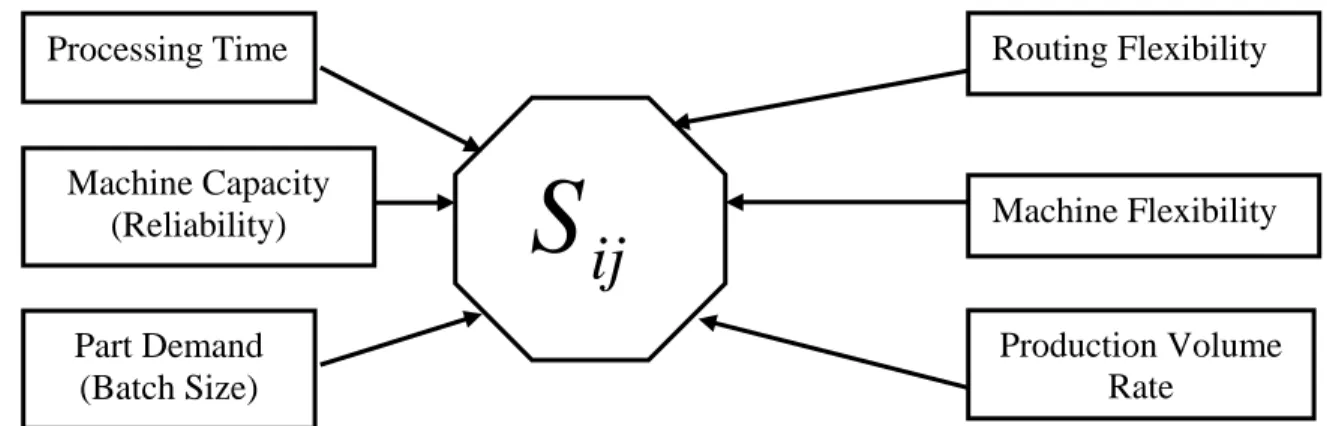
A comprehensive new similarity coefficient between machines will be created by considering alternative routings, processing time, machine capacity (reliability), machine capability (flexibility), production volume, product (part) demand, and number of operations done on each machine (figure 1). A relationship between machines can be calculated by using their similarity coefficient. The relationship between machines usually ranges from 0 to 1, as most researchers range as a function of the definition of a coefficient. As the value of the similarity coefficient approaches 1 , the two machines become more similar. If this value is equal to 0, there is no similarity between them. The main objective for creating the new similarity coefficient between machines is to take both direct and indirect relations between them into consideration.

The mathematical expression for the new similarity coefficient between machines i and j, which was based on machine capacity, machine flexibility (maximum number of operations available per machine), part (product) volume and demand, number of operations performed by machines, and processing time, will be explained as follows (see equations (37) and (38)).

Assumptions:

The model assumes that the following information has been collected and screened for accuracy or specified by the user.

1. The processing times for all part type operations with associated process plans on different

machine types are known.

(15)

3. The capability of each machine type is also known and constant over time.

4. Each machine type can perform one or more operations.

5. The production volume of each part type in a specific period is known.

6. The demand for each part type in the specific period is also known.

7. The production volume per part is greater than part demand.

Figure 1. Issues that will be used to create a new similarity coefficient between machines.

max max

/

max max max

1 max , max , X ijkr j i i j j i i

i j i

n _R

o o kjr

kir k

ijkr

i o j o k

k r ki and r kj ij

R R

o

o kjr o kjr

kir k kir

ijkr

i o j o k i o j

r ki r ki

and or

r kj r kj

n

n t

t V

X

C N C N D

S

n

n t n t

t V t

X OR

C N C N D C N C

= ∈ ∈ ∈ ∈ ∈ ∈ ⎡ ⎛ ⎞ ⎤ ⎢ ⎜ × × ⎟ ⎥ ⎜ ⎟ ⎢ _⎝ _⎠ ⎥ ⎣ ⎦ = ⎡ ⎛ ⎞ ⎤ ⎢ ⎜ × × ⎟ ⎥ + × ⎜ ⎟ ⎢ _⎝ _⎠ ⎥ ⎣ ⎦

∑ ∑

∑

max 1 1

Xijkr Xijkr

j j X ijkr

n n n

o _k

ijkr

o k

k k n

n _V Y N D − = = + ⎡⎛ ⎞ ⎤ ⎢⎜ × ⎟ ⎥ ⎜ ⎟ ⎢_⎝ _⎠ ⎥ ⎣ ⎦

∑

(37) or

(

)

(

)

(

)

∑

∑ ∑

∑∑

= − + = ∈ ∈ ∈ ∈ = ∈ ∈ ⎥ ⎥ ⎦ ⎤ ⎢ ⎢ ⎣ ⎡ ⎟ ⎟ ⎠ ⎞ ⎜ ⎜ ⎝ ⎛ × × + ⎥ ⎥ ⎦ ⎤ ⎢ ⎢ ⎣ ⎡ ⎟ ⎟ ⎠ ⎞ ⎜ ⎜ ⎝ ⎛ × × ⎥ ⎥ ⎦ ⎤ ⎢ ⎢ ⎣ ⎡ ⎟ ⎟ ⎠ ⎞ ⎜ ⎜ ⎝ ⎛ × × = ijkr

X Xijkr

ijkr X j j i i j j i i ijkr X j j i i n k k n n n k ijkr o o j kjr o o i kir R kj r orrki k ijkr o o j kjr o o i kir R kj r andki r n k k ijkr o o j kjr o o i kir R kj r andki r ij BS Y N n C t OR N n C t BS X N n C t N n C t BS X N n C t N n C t S 1 1 1 max max / max max max max , max , max (38) ij

S

kir

t processing time part k takes on machine i including setup time with process plan r

kjr

t processing time part k takes on machine j including setup time with process plan r

i

o

n number of operations done on machine i

j

o

n number of operations done on machine j

max

i

o

N

maximum number of operations available on machines i

max

j

o

N

maximum number of operations available on machine j

ij

S

Processing Time

Production Volume

Rate

Machine Capacity

(Reliability)

Routing Flexibility

Part Demand

(Batch Size)

Machine Flexibility

(16)

i

C

capacity of machine i

j

C

capacity of machine j

k

V

part volume of part type k per period

k

D

part demand of part type k per period

k

BS

batch size of part k

ijkr

X

=1 if part type k visits both machines i and j with process plan r

ijkr

X

=0 otherwise

ijkr

Y =1 if part type k visits either machine i or machine j with process plan r

ijkr

Y =0 otherwise

k = 1,…, n (parts), l = 1,…, m (machines), r = 1,…, R (routings)

R

number of part routings that can be processed on both machines i and j

\

R

number of part routings that can processed on either machine i or machine j

m number of machines in the machine-part incidence matrix.

n number of parts R in the machine-part incidence matrix.

ijkr

X

n number of parts that can visit both machines i and j with process routings r

i kir

C t

fraction of processing time which part k will take from the capacity of machine i

j kjr

C

t

fraction of processing time which part k will take from the capacity of machine j

max

i i

o o

N

n

number of operations done on machine i with respect to the maximum number of

operations available on that machine. This term represents the flexibility of machine i

max

j j

o o

N

n

number of operations done on machine j with respect to the maximum number of

operations available on that machine. This term represents the flexibility of machine j

k k

D V

ratio of production volume rate to demand per part

4. HEURISTIC APPROACH FOR MACHINE CELL FORMATION

Machines are assigned to machine cells based on our new similarity coefficient. The procedure to group machines into cells is given by the following steps:

Step 1: Check the Machine Work Load (MWL) of each machine type capacity (

C

i

,...,

C

m) to

produce all production volumes for all parts (

V

1

,...,

V

n) by these machines in the

machine-part incidence matrix. The MWL of machine i is based on production volumes and

processing times of all parts assigned to machine i. The equation for computing the MWL

(17)

(

)

∑ ∑

= ∈ ⎟

⎟ ⎠ ⎞ ⎜

⎜ ⎝ ⎛

+ + + = n

k

k ki k

ki k ki k

ki r r r

i t V t V t V

MWL

r r r

r r

ir

r 1 , ,

... max

2 1 2

1

(39)

Step 2: Compute the similarity coefficient matrix between all machine pairs according to equations (37) and (38).

Step 3: Determine the desired number of machines cells (NMC) by the following equation:

max

m

NMC

≥

m number of machines in machine-part incidence matrix.

max

m

pre-determinable maximum number of machines in the machine cell (at least two

machines per cell)

Step 4: Select the largest similarity coefficient between machine i and machine (j,…,m) from the similarity coefficient matrix in each row directly.

Step 5: Sort the similarity coefficients from highest to lowest value and record the values of

S

h and

the corresponding sets of

m

h

{

i

,

j

}

, where h represents the level of the similarity value.

Step 6: Start forming the first machine cell MC1 by selecting the highest similarity coefficient.

valueS₁. Then, this pair of machines m₁{i, j}will be clustered into the first machine cell.

Step 7: Check the minimum machine cell size constraint (at least two machines per cell).

Step 8: Increase the value of h (h = 2,…, H).

Step 9: If

m

h

I

MC

1

≠

0

. Then, modify MC1 by the new

MC

1

=

MC

1

U

m

h.

Otherwise, form a new machine cell

MC

n

(

n

=

2 ,...,

NMC

)

.

Step 10: If any set

m

h intersects two cells MCI and

MC

J, then, discard the corresponding

S

h and go back to Step 8.

Step 11: Check for the maximum number of machines allowed in a machine cell.

If the number of machines in this machine cell does not exceed the desired number of machines, then, add to this cell.

Otherwise, stop adding to this cell and go back to Step 8.

Step 12: If all the machines have not been assigned to machine cells, go back to Step 8. Otherwise, go to Step 13.

Step13: If the number of machine cells formed exceeds the desired number of machine cellsNMC, join two machine cells into one machine cell. All these steps will be shown in Figures 2 and 3.

(18)

5. ANALYTICAL EXAMPLE

In order to demonstrate the proposed approach, the following numerical example will illustrate the procedure, including the similarity coefficients and formation of machines into machine cells. It is composed of 10 types of machines and seven types of parts with different process plans. The incidence matrix between machines and parts is presented in table 1. The part information including operation sequence and processing times for each process plan, and production volume and part demand is also presented in table 2. Information about machine availability, including the capacities of the machines, number of operations that will be done on machines, and maximum number of operations available on machines, is shown in table 3.

Table 1. Incidence matrix between machines and parts.

Machine

Parts

P1 P2 P3 P4 P5 P6 P7

r11 r12 r21 r22 r23 r31 r32 r41 r51 r52 r61 r62 r71 r72

M1 1 0 1 1 0 1 0 0 0 1 0 1 0 0

M2 0 1 1 0 1 0 0 1 0 1 1 0 0 1

M3 0 1 0 1 1 0 1 0 1 0 0 0 1 0

M4 1 0 1 1 0 1 0 1 0 0 1 0 0 1

M5 1 0 1 0 1 0 1 0 0 0 0 0 0 0

M6 0 1 1 1 0 0 0 1 1 0 0 0 0 1

M7 1 0 0 0 1 1 0 0 1 1 1 0 0 0

M8 0 1 0 0 1 1 1 0 1 0 0 1 1 0

M9 0 1 0 1 0 1 1 1 0 1 0 1 0 1

(19)

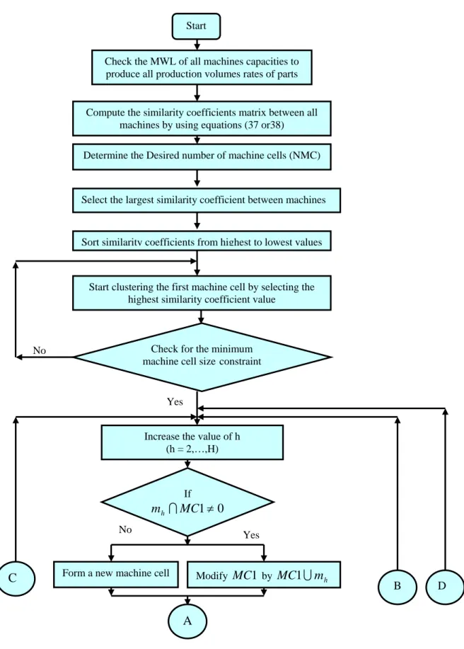
Figure 2. Flow chart of grouping machines into machine cells (Part 1).

Check the MWL of all machines capacities to

produce all production volumes rates of parts

Compute the similarity coefficients matrix between all machines by using equations (37 or38)

Determine the Desired number of machine cells (NMC)

Select the largest similarity coefficient between machines

Start clustering the first machine cell by selecting the highest similarity coefficient value

Sort similarity coefficients from highest to lowest values

Check for the minimum machine cell size constraint No

Yes

Increase the value of h (h = 2,…,H)

Form a new machine cell If

0

1 ≠

MC

m

_h

_I

Modify MC1 by

MC

1 U

m

h

Yes No

D

Start

A

B

(20)

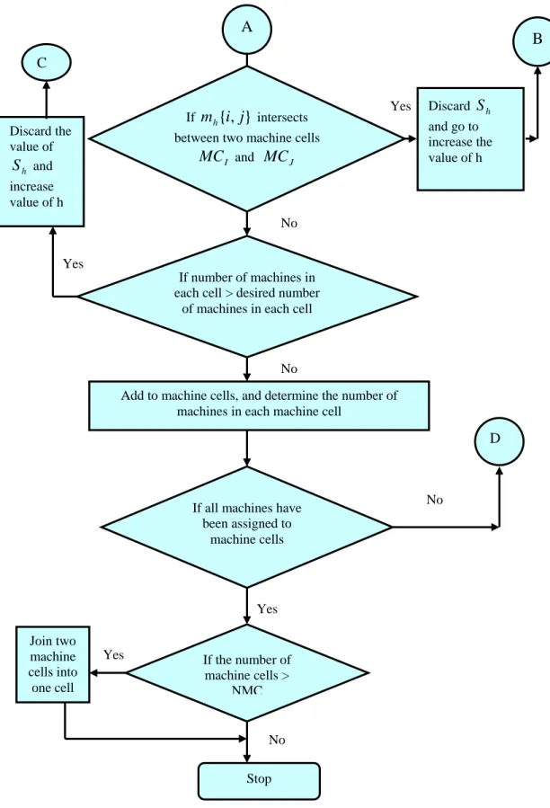
Figure 2. Flow chart of grouping machines into machine cells (Part 2).

No

Yes

No

Yes

No Yes

Join two machine cells into one cell

Stop

Discard

S

_h

and go to increase the value of h If

m

h

{

i

,

j

}

intersects

between two machinecells

I

MC and

MC

_J

If number of machines in each cell > desired number

of machines in each cell

C

Add to machine cells, and determine the number of machines in each machine cell

If all machines have been assigned to

machine cells

D

If the number of machine cells >

NMC Discard the

value of

h

S

and increase value of h

A

(21)

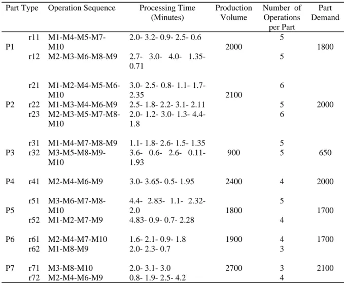
Table 2. Parts information.

Part Type Operation Sequence Processing Time

(Minutes)

Production Volume

Number of Operations per Part

Part Demand

P1

r11 M1-M4-M5-M7-M10

2.0- 3.2- 0.9- 2.5- 0.6

2000

5 1800

r12 M2-M3-M6-M8-M9 2.7- 3.0- 4.0- 1.35- 0.71

5

P2

r21 M1-M2-M4-M5-M6-M10

3.0- 2.5- 0.8- 1.1- 1.7-

2.35 2100

6 2000

r22 M1-M3-M4-M6-M9 2.5- 1.8- 2.2- 3.1- 2.11 5

r23 M2-M3-M5-M7-M8-M10

2.0- 1.2- 3.0- 1.3- 4.4- 1.8

6

P3

r31 M1-M4-M7-M8-M9 1.1- 1.8- 2.6- 1.5- 1.35

900

5 650

r32 M3-M5-M8-M9-M10

3.6- 0.6- 2.6- 0.11- 1.93

5

P4 r41 M2-M4-M6-M9 3.0- 3.65- 0.5- 1.95 2400 4 2000

P5

r51 M3-M6-M7-M8-M10

4.4- 2.83- 1.1- 2.32-

2.0 1800

5 1700

r52 M1-M2-M7-M9 4.83- 0.9- 0.7- 2.28 4

P6 r61 M2-M4-M7-M10 1.6- 2.1- 0.9- 1.8 1900 4 1700

r62 M1-M8-M9 2.0- 2.3- 0.7 3

P7 r71 M3-M8-M10 2.0- 3.1- 3.0 2700 3 2100

r72 M2-M4-M6-M9 0.8- 1.9- 2.5- 4.2 4

Table 3. Machine information. Machine

Type

Capacity of machine

(Hours)

Number of Operations done on

machine (

n

o)

Maximum number of operations available on machine

(

N

max)

1 2400 6 6

2 2000 7 7

3 2300 6 6

4 3000 7 10

5 1800 4 4

6 1900 6 9

7 2700 6 8

8 1300 7 10

9 2500 8 9

(22)

5.1. Similarity Coefficient between Machines

The similarity coefficient between machines has been coded in the C programming language and executed on a Pentium IV processor. The result of similarity coefficients between machines is illustrated in table 4.

5.2. Machine Cells Formation

Step 1: Check the capacity of each machine type (availability of time per machine) to produce all parts that require processing on the machine.

For machine one (M1), the capacity for M1 equals 2400 hours. The total consumed time taken from M1 will be calculated as follows:

hours 4 . 396 60

784 , 23

)] 1900 ( 0 . 2 ) 1800 ( 83 . 4

) 900 ( 1 . 1 ) 2100 ( 5 . 2

) 2100 ( 0 . 3 max[ ) 2000 ( 2

60

1 ₌ ₌

⎥ ⎥ ⎥ ⎦ ⎤ ⎢

⎢ ⎢ ⎣ ⎡

+

+ +

The slack of time on machine (M1) is 2400-396 = 2004 hours. So, M1 is OK. The slack of time on machine (M2) is 2000-412 = 1588 hours. So, M2 is OK. The slack of time on machine (M3) is 2300-439 = 1861 hours. So, M3 is OK. The slack of time on machine (M4) is 3000-509 = 2491 hours. So, M4 is OK. The slack of time on machine (M5) is 1800-144 = 1656 hours. So, M5 is OK. The slack of time on machine (M6) is 1900-453 = 1447 hours. So, M6 is OK. The slack of time on machine (M7) is 2700-229 = 2471 hours. So, M7 is OK. The slack of time on machine (M8) is 1300-440 = 860 hours. So, M8 is OK. The slack of time on machine (M9) is 2500-475 = 2025 hours. So, M9 is OK. The slack of time on machine (M10) is 2100-383 = 1716 hours. So, M10 is OK. The capacities of all machines are satisfy to all production volumes for all parts.

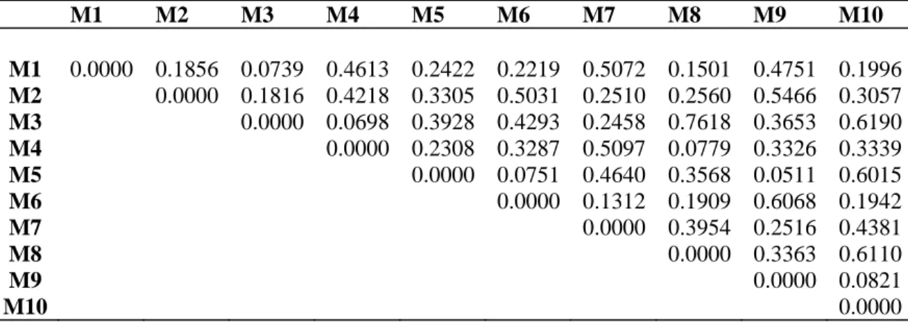
Step 2: Compute the similarity coefficient matrix between all machines according to the similarity coefficient (37).

Table 4. Similarity coefficients between machines.

M1 M2 M3 M4 M5 M6 M7 M8 M9 M10

M1 0.0000 0.1856 0.0739 0.4613 0.2422 0.2219 0.5072 0.1501 0.4751 0.1996

M2 0.0000 0.1816 0.4218 0.3305 0.5031 0.2510 0.2560 0.5466 0.3057

M3 0.0000 0.0698 0.3928 0.4293 0.2458 0.7618 0.3653 0.6190

M4 0.0000 0.2308 0.3287 0.5097 0.0779 0.3326 0.3339

M5 0.0000 0.0751 0.4640 0.3568 0.0511 0.6015

M6 0.0000 0.1312 0.1909 0.6068 0.1942

M7 0.0000 0.3954 0.2516 0.4381

M8 0.0000 0.3363 0.6110

M9 0.0000 0.0821

(23)

Step 3: Determine the desired number of machine cells, NMC. The maximum number of machines assigned to cells ranged from 3 to 7 machines (Wilhelm et al. 1998) and from 5 to 10 machines (Ramabhatta and Nagi 1998). Four machines per cell are recommended for easy management and control.

5 .

2

4

10 ≥

≥

NMC

. Therefore, the number of machine cells can start with three cells.

Three machine cells will be chosen.

Step 4: Select the largest similarity coefficient between machine i and machine (j,…,m) from Table 4 as follows:

7 1

m

−

0.5072

9 2

m

−

0.5466

8 3

m

−

0.7618

7 4

m

−

0.5097

10 5

m

−

0.6015

9 6

m

−

0.6068

10 7

m

−

0.4381

10 8

m

−

0.6110

10 9

m

−

0.0821

Step 5: Sort the similarity coefficients from the highest to lowest value and record the values of

S

_h

and the corresponding sets of

m

_h

{

i

,

j

}

H

m

_h

{

i

,

j

}

S

_h

____________ ______

1

m

₃

−

m

₈ 0.7618

2

m

₈

−

m

₁₀ 0.6110

3

m

₆

−

m

₉ 0.6068

4

m

₅

−

m

₁₀ 0.6015

5

m

₂

−

m

₉ 0.5466

6

m

₄

−

m

₇ 0.5097

7

m

₁

−

m

₇ 0.5072

8

m

₇

−

m

₁₀ 0.4381

Step 6: For S₁= 0.7618 (between Machines 3 and 8).

(24)

Step 7: Check the minimum machine cell size constraint (at least two machines per cell).

Step 8: S₂= 0.6110 (between Machines 8 and 10).

2

m = {8, 10}

Step 9: There is an intersection between Machine 8 andMC₁.

The new machine cell isMC1Um2.

Then, the revised machine cell MC₁= {3, 8, 10}

3

S

=0.6068 (between Machines 6 and 9)

3

m

= {6, 9} and

MC

1

I

m

3

=

0

3

S

does not intersect with MC1

Then, form a new machine cell MC2= {6, 9}

4

S = 0.6015 (between Machines 5 and 10)

4

m = {5, 10}

There is an intersection between Machine 10 andMC₁, but there is no intersection withMC₂.

The new machine cell isMC1Um4.

Then, the revised machine cell

1

MC = {3, 5, 8, 10}

Step 10: Check for the maximum number of machines a machine cell.

Machine Cell 1 contains four machines. Therefore, no more machines are added to MC1.

5

S

= 0.5466 (between Machines 2 and 9)

5

m

= {2, 9}

There is an intersection between Machine 9 andMC₂, but this is no intersection withMC₁_{. The}

new machine cell is

MC

₂

_U

m

₅.

Then, the revised machine cell MC₂= {2, 6, 9}

6

S

6

m

={4,7},

MC

1

I

m

6

=

0

,and

MC

2

I

m

6

=

0

There is no intersection between Machines 4 or 7 with eitherMC1 orMC2.

Then, forms a new machine cell

MC

₃= {4, 7}

7

S

7

m

= {1, 7}

There is an intersection between Machine 7 and

MC

₃_{, but this is no intersection with} MC₁

orMC₂_{. The new machine cell is}

MC

₃

_U

m

₇.

Then, the revised machine cell

MC

₃= {1, 4, 7}

(25)

Machine Cells are as follows:

1

MC = {3, 5, 8, and 10} 2

MC = {2, 6, and 9} 3

MC

= {1, 4, and 7}

6. CONCLUSIONS

This paper proposed a new similarity coefficient for grouping machines into machine cells. Similarity coefficients between machines were reviewed through this paper. These similarity coefficients show that there are several factors or issues to be used in determining the similarity between machines. Some of them concentrated on the machine–part incidence matrix, and the rest of them depend on one or two production and/or flexibility issues like production volume, operation sequence, part demand, and number of intercellular moves. This variation will lead to suggest a new comprehensive similarity coefficient between machines including the most important production and flexibility issues. The main difference between the proposed similarity coefficient and those which already existed in the literature is the lack of them to incorporate all the real world issues. The results in table 4 showed how each value of the similarity coefficient is different. The heuristic based similarity approach was used to group machines into machine cells.

REFERENCES

[1] Aljaber N., Baek W., Chen C.L. (1997), A Tabu search approach to the cell formation

problem; Computers & Industrial Engineering 32; 169-185.

[2] Chang P. T., Lee E.S. (2000), A multisolution method for cell formation-exploring practical

alternatives in group technology manufacturing; Computers and Mathematics with

Applications 40; 1285-1296.

[3] Gunasingh K.R., Lashkari R.S. (1989), Machine grouping problem in cellular manufacturing

systems: An integer programming approach; International Journal of Production Research

27; 1465-1473.

[4] Gupta T. (1991), Clustering algorithms for the design of a cellular manufacturing system-An

analysis of their performance; Computers & Industrial Engineering 20; 461-468.

[5] Gupta T. (1993), Design of manufacturing cells for flexible environmental considering

alternative routing; International Journal of Production Research 31; 1259-1273.

[6] Gupta T., Seifoddini H. (1990), Production data based similarity coefficient for

machine-component grouping decisions in the design of a cellular manufacturing system; International

Journal of Production Research 28; 1247-1269.

[7] Islam K.M.S., Sarker B.R. (2000), A similarity coefficient measure and machine-parts

grouping in cellular manufacturing systems; International Journal of Production Research

38; 699-720.

[8] Lee M.K., Luong H.S., Abhary K. (1997), A genetic algorithm based cell design considering

(26)

[9] Leem C.-W., Chen J.J. G. (1996), Fuzzy-set-based machine-cell formation in cellular

manufacturing; Journal of Intelligent Manufacturing 7; 355-364.

[10] Lozano S., Canca D., Guerrero F., Garcia J.M. (2001), Machine grouping using sequence

based similarity coefficients and neural network; Robotics and Computer Integrated

Manufacturing 17; 399-404.

[11] Luong L.H.S. (1993), A cellular similarity coefficient algorithm for the design of

manufacturing cells; International Journal of Production Research 31; 1757-1766.

[12] Luong L.H.S., Kazerooni M., Abhary K. (2001), Genetic algorithms in manufacturing system

design. In Computational Intelligence in Manufacturing Handbook, edited by Jun Wang et

al., Boca Raton, FL (CRC Press LLC).

[13] McAuley J. (1972), Machine grouping for efficient production; The Production Engineer 52;

53-57.

[14] Mosier C. (1989), An experiment investigating the application of clustering procedures and

similarity coefficients to the GT machine cell formation problem; International Journal of

Production Research 27; 1811-1835.

[15] Nair G.J., Narendran T.T. (1998), CASE: A clustering algorithm for cell formation with

sequence data; International Journal of Production Research 36; 157-179.

[16] Nazarlo D., Ramirez B. (2000), Application of mixed integer programming to cellular

manufacturing; Engineering Valuation and Cost Analysis 2; 373-386.

[17] Ponnambalam S.G., Aravindan P. (1994), Design of cellular manufacturing systems using

objective functional clustering algorithms; International Journal of Advanced Manufacturing

Technology 9; 390-397.

[18] Probhakaran G., Janakiraman T.N., Sachithanandam M. (2002), Manufacturing data-based

combined dissimilarity coefficient for machine cell formation; International Journal of

Advanced Manufacturing Technology 19; 889-897.

[19] Ramabhatta V., Nagi R. (1998), An integrated formulation of manufacturing cell formation

with capacity planning and routing; Annals of Operations Research 77; 79-95.

[20] Seifoddini H. (1988), Incorporation of the production volume in machine cells formation in

group technology applications. Recent Developments in Production Research, edited by A. Mital, (Elsevier Science Publishers B.V., Amsterdam), 562-570.

[21] Seifoddini H. (1989), A probabilistic approach to machine cell formation in group

technology. International Conference of Institute of Industrial Engineers, Toronto, Ontario, Canada, May 14-17, 625-629.

[22] Seifoddini H., Djassemi M. (1991), The production data-based similarity coefficient versus