Reliable location-allocation model for congested systems under
disruptions using accelerated Benders’ decomposition
Naeme Zarrinpoor1, Mohammad Saber Fallahnezhad1*, Mir Saman Pishvaee2
1
Department of industrial engineering, Yazd University, Yazd, Iran
2
Department of industrial engineering, Iran University of Science and Technology, Tehran, Iran
[email protected], [email protected], [email protected]
Abstract
This paper aims to propose a reliable location-allocation model where facilities are subject to the risk of disruptions. Since service facilities are expected to satisfy random and heavy demands, we model the congested situations in the system within a queuing framework which handles two sources of uncertainty associated with demand and service. To insure the service quality, a minimum limit reflected in the customers’ expected waiting time is considered in the model. We also consider the geographical accessibility of the service network in terms of the proximity of a facility to the potential demands. The model determines the optimal number and locations of facilities and the corresponding customer assignments in such a way as to minimize the fixed installation cost as well as expected traveling, serving and penalty costs. To obtain exact solution of the proposed model, a Benders’ decomposition algorithm enhanced by two efficient accelerating methods including valid inequalities and knapsack inequalities is proposed. Numerical results illustrate the applicability of the proposed model as well as the effectiveness of the designed solution procedure.
Keywords: Location-allocation model, disruption, queuing system, service quality, geographical accessibility, Benders’ decomposition
1- Introduction
Location-allocation models deal with finding the location of new facilities in some given geographical areas and the allocation of demand nodes to the located facilities in such a way as to minimize total travel time, physical distance, operational or transportation costs or to maximize the market capture or reliability (Boffey et al., 2006; Zarrinpoor and Seifbarghy, 2011).Beginning from the study of Weber (1909), numerous researches have been developed for facility location problem. The exhaustive reviews in this area were provided by Revelle et al.,(2005) and Revelle et al.,(2008).
A common assumption in classical facility location problems is that built facility will remain operational forever. However, in practice there are many types of disruptive events which can make the facility unavailable
*Corresponding author.
ISSN: 1735-8272, Copyright c 2016 JISE. All rights reserved Journal of Industrial and Systems Engineering
Vol. 9, special issue on location allocation and hub modeling, pp 100-117 Winter (February) 2016
from a time moment to another one. Disruptive events may be originated from different reasons including natural disasters, equipment breakdowns, terrorist attacks, labor strikes, changes in ownership, etc (Snyder and Daskin, 2005). In the occurrence of disruptions, it is impossible to immediately change the network substructure to serve demands. Often, in order to achieve system reliability, mitigation or recourse operation is implemented in such a way as to reassign the demand nodes to other operational facilities much farther than their regularly assigned facilities (Snyder and Daskin, 2005; Aydin and Murat, 2013). Facility disruptions can significantly deteriorate the overall system efficiency and responsiveness. Therefore, it is crucial to design a reliable network that can work properly in both normal and disruptive conditions.
Generally, real service facilities are expected to meet heavy and random demands. Since facilities have not enough capacity to serve all the simultaneous demands immediately, the system may be congested in some situations. To study the probabilistic nature of demand and service of such systems, the incorporation of queuing theory into the facility location has gained much attention recently. Some examples of congested systems include post offices, bank branches, automated teller machines, vending machines, check-in counters in airports, checkout counters in stores, proxy/mirror servers in communication networks, emergency medical service, healthcare facilities and distribution centers in supply chains(Wang et al.,2002;Huang et al.,2005;Aboolian et al.,2009). Precisely, in the disruptive conditions we might expect a higher level of congestion in the system. Consequently, to obtain a more reliable configuration of real service network, congestion must be considered in service facility location and allocation decisions.
Since location and allocation decisions are the most important strategic decisions in numerous contexts such as supply chain planning, transportation infrastructure design and public service systems, different fundamental issues must be considered in the modeling to design an efficient and effective service network design, including reliability aspects, risk of disruptions, congestion, geographical accessibility and corresponding costs. Regarding the literature (See section 2), there is no comprehensive model that considers all the aforementioned aspects. The current research proposes a location-allocation model where facilities are subject to the risk of disruptions. The uncertainty associated with demand as well as service is considered in the model within the queuing system. The geographical accessibility of a service network is considered in terms of the proximity of a facility to the potential customers. To solve the proposed model, a Benders’ decomposition algorithm enhanced by two accelerating methods including valid inequalities and knapsack inequalities is proposed. Several generated instances are presented to illustrate the applicability of the developed model as well as the effectiveness of the designed solution procedure.
The rest of the paper is organized as follows. The next section reviews the related literature. Section 3 presents the mathematical model. In Section 4, an accelerated Benders decomposition is developed to solve the model. Section 5 describes several generated instances to illustrate the applicability of the proposed model. Section 6 ends with some conclusions and possible directions for future research.
2- Literature review
The relevant literature in two separate but complementary research streams in the context of facility location problem is reviewed in this section and then the main contributions of this research are presented.
2-1- Facility location problem under disruptions
The earliest study of reliable facility location problem dates back to the work of Drezner (1987), who formulated p-median problem (PMP) under the assumption that some facilities may become inactive, and (p,q)-center problem in which p facilities need to be located and at most q facilities may become inactive. Snyder and Daskin (2005) presented reliability-based formulations of PMP and uncapacitated fixed-charge location problem (UFLP) with equal facility failure probability. Berman et al,. (2007) considered the PMP with independent failure probabilities under the complete information of customers about the operational status of facilities. For site-dependent random facility disruptions, Cui et al. (2010) proposed a compact mixed integer program formulation to study the reliable UFLP and developed both Lagrangian relaxation and continuum approximation methods to solve it. Li and Ouyang (2010) addressed the UFLP under correlated and site-dependent facility disruptions and formulated the proposed model upon the continuum approximation approach. Lim et al., (2010) studied the reliable facility location problem in the presence of random facility disruptions with the option of hardening selected facilities. Shen et al., (2011) proposed both scenario-based stochastic programming and a nonlinear mixed integer programming models for a reliable facility location problem considering unequal failure
probabilities. Peng et al., (2011) used the p-robustness criterion to develop a reliable model for designing a logistic network under facility failures. Chen et al., (2011) incorporated inventory management decisions into the facility location design framework assuming that facilities are subject to the equal probabilistic facility failures. The reliable capacitated facility location problem was addressed by Aydin and Murat (2013) who formulated the problem as a two-stage stochastic program. In the context of competitive facility location problem, Wang and Ouyang (2013) proposed game-theoretical models based on continuum approximation approach in which spatial competition and probabilistic facility disruption are considered. Interdependent and correlated failures in facility location problem within a supporting structure framework for an infrastructure system were considered by Li et al., (2013a). The impact of misestimating the disruption probability in the reliable facility location model was studied by Lim et al., (2013). Li et al., (2013b) introduced the reliable PMP and UFLP under heterogeneous facility failure probabilities and facility fortification within a finite budget. An et al., (2014) adopted a two-stage robust optimization approach to study both cases of reliable capacitated and un-capacitated PMP. Alcaraz et al., (2015) presented a set packing formulation of the reliable UFLP and studied certain aspects of its polyhedral properties by identifying a number of clique facets. Yun et al. (2015) proposed a reliable facility location model under independent and identical facility disruptions and assumed that customer does not have complete information about the operational status of facilities. Zhang et al., (2016) studied a reliable location-inventory model in which facilities may fail with heterogeneous disruption probabilities.
2-2- Facility location for congested systems
A facility location problem for congested systems was addressed first by Berman and Larson (1985). Marianov and Serra (1998) presented several maximal coverage models under constrained waiting time and queue length. Several queuing location-allocation models with hierarchical structure were addressed by Marianov and Serra (2001). Wang et al., (2002) studied a facility location problem by considering the queuing system which minimizes the expected total traveling and waiting times. Marianov (2003) presented a location model of congested facilities to maximize expected demands. Shavandi and Mahlooji (2006) presented a fuzzy queuing location-allocation model which maximizes the total covered demands. Syam (2008) developed a multiple server location–allocation model for service system design. Marianov et al., (2008) addressed a competitive facility location model in which customers choose the facilities they patronize, by the travelling and waiting times. Zhang et al., (2009) considered congestion situation in the preventive healthcare facility network design. Aboolian et al., (2009) investigated a multiple server location problem that minimizes the maximum time spent at the server sites, including travelling and waiting times. Zarrinpoor and Seifbarghy (2011) proposed a model for congested systems in which a new entering firm desires to obtain a specific percentage of the market share in such a way as to minimize the total costs. More recently, Rahmati et al.,(2013), Hajipour et al., (2014) and Hajipour et al.,(2016) proposed either bi-objective or multi-objective facility location models with different queuing systems and applied some evolutionary algorithms to solve them.
2-3- Contributions of this research
Regarding the literature, we can conclude that there is no research that considered reliability aspects for service facilities which are expected to satisfy heavy and random demands and due to their limited capacity, the system may be congested in some situations. Although the geographical accessibility of facilities is one of the most important factors in the success of the service network design, no research work considered it in the modeling. Moreover, the un-capacitated models have been gained more attention compared with capacitated ones. However, their applications in the practical contexts have limited due to their unrealistic assumption. The approximation or meta-heuristic algorithms are the main solution procedures in the most of presented research papers and exact solution algorithms have been received less attention.
This paper proposes a location-allocation model for service facilities in which both congestion and reliability are considered concurrently. To cope with congested situations, an M/G/1 queuing system is investigated which assists to model two source of uncertainty associated with demand and service. The geographical accessibility and service quality restrictions are also considered in the model to design an effective and efficient service network. An accelerated Benders decomposition algorithm is presented which seeks to find exact solution of the proposed model.
3-Problem formulation
In this section, we present the notation and formulation of reliable facility location-allocation model for congested systems under disruptions.
3-1- Notation
The sets, parameters, and decision variables used in the proposed model are defined as follows: Sets
Set of demand nodes
Set of candidate locations for facilities Set of assignment levels
Parameters
Fixed installation cost to establish facility at candidate location ∈ Transportation cost from demand node ∈ to facility ∈
Unit cost of serving customer residing at demand node ∈ by facility ∈ Shortest distance between demand node ∈ and facility ∈
Maximum acceptable distance for demand nodes to access the service of facilities
ℎ Demand rate at demand node ∈
Total arrival rate at facility ∈ Service rate of facility ∈
Variation of service time at facility ∈
Customers’ expected waiting time at facility ∈
Maximum acceptable customers’ waiting time at facility ∈ Q Failure probability of each facility
Maximum number of facilities that can be established Decision variables
1 if a facility is located at node ∈ , 0 otherwise
Portion of customers residing at demand node ∈ is assigned to facility ∈ at assignment level ∈
3-2- Formulation
The system under study is represented as a network where arcs are the possible paths between nodes and nodes represent either candidate location for facilities or demand concentrations. The service facilities are expected by system designers to remain operational forever. However, the system may become unavailable due to the disruptive events caused by natural disasters or man-made hazards from a time moment to another one (Snyder and Daskin, 2005; An et al., 2014). To cope with such situations, we assume that each facility may fail independently with an identical failure probability . In the occurrence of disruption, the facility cannot provide any service and its customers will be reassigned to other operational facilities. We assume that each customer can get service from ≤ | | facilities.For a customer residing at node , a “level-r” assignment is used when all its assigned facilities at levels 1, … , − 1 have failed and th facility can provide service for customer.Therefore, the probability that a customer can receive service at level-r assignment is defined as follows:
p%serving customer at level − r assignment4 = %1 − q4q789%14
Note that in normal disruption-free situation, a customer will be assigned to level-1 facility. If all assigned facilities to the customer have failed, the customer gives up service and the system will incur a penalty cost. It is worth mentioning that the probability of incurring penalty cost is :. To model the congested situations, we assume that each facility behaves as an M/G/1queue implying that the requests for the service appear according to a Poisson process and the service time has a general distribution. It should be noted that the Poisson process is a good representation of the arrival rates of real-world service networks in which there is always a variation around scheduled times. It can also be generalized to other service systems where arrival rates and capacity levels vary significantly over time, as pointed out by many researchers such as Nosek and Wilson (2001), Preater (2002), Green (2006), Zhang et al.(2009) and Zhang et al.,(2012). Moreover, in a general probability distribution
for service time, no assumption is made as to the precise form of the distribution. Therefore, results in these cases are applicable to any probability distribution, as pointed out by Gross and Hariss (1988).
Considering the M/G/1queuing system, the demand generation rate at each demand node iis the Poisson process with average demand rate ℎ, thus the demand rate at facility j can be written as:
λ<= = = h? 7∈@ ?
x?<7. %24
Since is a linear combination of Poisson processes, it is itself a Poisson process.
According to Gross and Hariss (1988), the customers’ expected waiting times at facility is the following w<= E1 + CV<
I
2 Jμ<ρ− λ< <+
1
μ<. %34
where N = ⁄ and PQ = . With respect to the definitions of N and PQ, we can rewrite the above equation as follows:
w<= E1 + σ<
Iμ
< I
2 Jμ<Sμ<λ− λ< <T+
1
μ<. %44
To maintain congestion within acceptable limit, a capacity constraint must be considered in the model. The common approach used to consider the capacity constraints in facility location problem is to force the demand for service at each facility not to exceed the maximum allowable capacity. Such a deterministic capacity constraint is not able to reflect the dynamic nature of congestion in which the number of requests for service is not constant in time and behaves some probabilistic distributions. To deal with congestion, the expected number of requests for service or waiting time can be restricted to be less than some small values (Marianov and Serra, 1998; Marianov and Serra, 2001). Moreover, the quality of service network can be expressed in terms of expected or worst case waiting times or queue length for a specific service (Zhang et al., 2009; Zhang et al., 2012). Therefore, the service quality for facility is enforced throughrestriction on the level of congestion to ensure that customers’ expected waiting times in system do not exceed maximum acceptable level as the following:
w<≤ τ<y<. %54
By considering Eq. (4), the above equation can be stated as follows:
S1 + σ<Iμ<ITλ<+ 2μ<Sμ<− λ<T ≤ 2τ μ<Sμ<− λ<Ty< %64
The above equation can be rewritten in a simpler form as follows:
ZS1 + σ<Iμ<IT − 2μ<+ 2τ<μ<y<[λ<≤ 2μ<ISτ<− 1Ty< %74
As previously mentioned, geographical accessibility is one of the key elements for the success of service networks that can significantly affect the transportation network design. We consider it in the model in terms of the proximity of a facility to the potential demand nodes which specifies customer should not take more than amaximum acceptable travel distance to access service of facility . Therefore, we have
x?<7= 0, ∀ j ∈ `jad?<> ddefg. %84
For this service network, we are seeking a model that selects the location of facilities and allocates customers to the constructed facilities with consideration of queuing system and geographical accessibility in such a way as to minimize the fixed installation cost as well as the expected operational costs. By considering the aforementioned assumptions and queuing system representation, the formulation of reliable facility location-allocation model under disruptions can be stated as follows:
Min = f<y<+ <∈k
= = = h? 7∈@ <∈k ?∈l
c?<%1 − q4q789x?<7+ = = = h?
7∈@ <∈k ?∈l
s?<%1 − q4q789x?<7+ =Π?h?
?∈l
q@ %94
s.t. = x?<7= 1 <∈k , ∀i ∈ I, r ∈ R, %104
= x?<7≤ 1 7∈@ , ∀i ∈ I, j ∈ J, %114
x?<7≤ y<, ∀i ∈ I, j ∈ J, r ∈ R, %124 = y<≤ p <∈k %134
ZS1 + σ<Iμ<IT − 2μ<+ 2τ<μ<y<[ = = h? 7∈@ ?∈l x?<7≤ 2μ<ISτ<− 1Ty<, ∀j ∈ J, %144
x?<7= 0, ∀i ∈ I, j ∈ `jad?< > ddefg, r ∈ R, %154
y< = 0, 1, ∀j ∈ J, %164
x?<7≥ 0, ∀i ∈ I, j ∈ J, r ∈ R. %174
The Objective function (9) minimizes fixed installation cost, expected traveling cost from customers to the facilities, expected serving cost of customers by constructed facilities and expected penalty cost of unsatisfied demands. Constraint (10) insures that each customer is assigned to exactly one facility at each assignment level. Constraint (11) states no customer can be assigned to the same facility at two or more assignment levels. Constraint (12) specifies that a customer only assigned to the open facilities. Constraint (13) specifies maximum number of facilities that can be established. Constraint (14) ensures the service quality by considering maximum limit reflected in customers’ expected waiting time at each service facility. Constraint (15) ensures that customers should not take more than a maximum acceptable distance to access service at facilities. Constraint (16) and (17) enforce the binary and non-negativity restrictions on the corresponding decision variables. 3-3- Linearization of the proposed model Due to the multiplication of binary and integer variables in constraint (14), the proposed model is non-linear. By considering r = and M as a reasonably large number, the non-linear constraint can be replaced by st1 +σ<Iµ<Iu − 2µ<v = = h? 7∈@ ?∈l x?<7+ 2τ<µ<= = h? 7∈@ ?∈l Ω?<7≤ 2µ<ISτ<− 1Ty<, ∀j ∈ J, %184
Ω?<7≤ x?<7, ∀i ∈ I, j ∈ J, r ∈ R, %194
Ω?<7≤ My<, ∀i ∈ I, j ∈ J, r ∈ R, %204
Ω?<7≤ x?<7− MS1 − y<T, ∀i ∈ I, j ∈ J, r ∈ R, %214
Ω?<7≥ 0, ∀i ∈ I, j ∈ J, r ∈ R. %224
4- Solution procedure
The linearized proposed problem is a mixed integer programming (MIP) and it can be solved by current state-of-the-art MIP solvers. However, applying such solvers in solving large-scale instances requires significant computational time. The structure of proposed problem is a natural candidate to be solved by a well-known partitioning method, Benders decomposition (Benders, 1962). The successful application of this algorithm has been reported in different contexts such as supply chain network design (Pishvaee et al., 2014), scheduling
(Verstichel et al., 2015), hub location problem (Camargo et al., 2008) and facility location (Vatsa and Jayaswal, 2016).
4-1- Benders decomposition algorithm
To implement Benders’ decomposition procedure, the dual sub-problem (DSP) and master problem (MP) should be formulated. Let fix the binary variable to the given value`w = g. Then, the Benders primal sub-problem (PSP) can be formulated as follows:
Min PSP = = = = h? 7∈@ <∈k ?∈l
c?<%1 − q4q789x?<7+ = = = h?
7∈@ <∈k ?∈l
s?<%1 − q4q789x?<7 %234
s. t. %104, %114, %154, %174, %194, %224 x?<7≤ yw<∀i ∈ I, j ∈ J, r ∈ R %244
st1 +σ<Iµ<Iu − 2µ<v = = h? 7∈@ ?∈l x?<7+ 2τ<µ<= = h? 7∈@ ?∈l Ω?<7≤ 2µ<ISτ<− 1Tyw<∀j = 1, … , J %254
Ω?<7≤ Myw<, ∀i, j, r, %264
Ω?<7≤ x?<7− MS1 − yw<T, ∀i, j, r, %274
Let z , { , | , } , ~ , • , € , • , ‚ and ƒ be the vector of dual variables of the constraints (10), (11), (15), (17), (19), (22) and (24)-(27). The DSP can be stated as follows: Max DSP = = = ζ?7 7∈@ ?∈l − = = φ?< <∈k ?∈l − = = = ς?<7 7∈@ <∈k ?∈l yw<− 2 =µ<ISτ<− 1Tyw<ϑ< <∈k − M = = = ψ?<7 7∈@ <∈k ?∈l yw< + M = = =S1 − yw<T 7∈@ <∈k ?∈l ϖ?<7%284 s.t. ζ?7− φ?<+ ν?<7+ ξ?<7+ ϱ?<7− ς?<7− st1 +σ<Iµ<Iu − 2µ<v h?ϑ<+ ϖ?<7 ≤ h?c?<%1 − q4q789+ h?s?<%1 − q4q789 , ∀i ∈ I, j ∈ `jad?<> ddefg, r ∈ R %294
ζ?7− φ?<+ ξ?<7+ ϱ?<7− ς?<7− st1 +σ<Iµ<Iu − 2µ<v h?ϑ<+ ϖ?<7≤ h?c?<%1 − q4q789+ h?s?<%1 − q4q789 , ∀i
∈ I, j ∉ `jad?<> ddefg, r ∈ R %304
−ϱ?<7+ ϕ?<7− 2τ<µ<h?ϑ<− ψ?<7− ϖ?<7≤ 0, ∀i ∈ I, j ∈ J, r ∈ R, %314
φ?<, ξ?<7, ϱ?<7, ϕ?<7, ς?<7, ϑ<, ψ?<7, ϖ?<7≤ 0, ∀i ∈ I, j ∈ J, r ∈ R, %324
ζ?7, ν?<7 free, ∀i ∈ I, j ∈ J, r ∈ R %334
According to the solution of DSP, the MP can be written as follows: Min MP = = f<y<+ <∈k =Π?h? ?∈l q@+ η %344
η ≥ = = ζ?7ℓ 7∈@ ?∈l
− = = φ?<ℓ <∈k ?∈l
− = = = ς?<7ℓ 7∈@ <∈k ?∈l
yw<− 2 =µ<ISτ<− 1Tyw<ϑ<ℓ
<∈k
− M = = = ψ?<7ℓ 7∈@ <∈k ?∈l
yw<
+ M = = =S1 − yw<T 7∈@
<∈k ?∈l
ϖ?<7ℓ , ∀ℓ ∈ ’ %354
η ≥ 0 %364 It should be noted that MP produces an upper bound for the primary problem for each iteration. Constraint (35) represents the optimality cut, Szℓ, {ℓ, |ℓ , }ℓ , ~ℓ , •ℓ , €ℓ , •ℓ, ‚ℓ , ƒℓ T indicates the extreme point of dual polyhedron obtained by solving the DSP and ’ is the set of extreme points. The DSP is always feasible since the unmet demand is penalized. Therefore, the feasibility cut is not considered in the MP. The MP and DSP are solved iteratively by using the solution of one in the other, until the stopping criterion is met and an optimal solution can be obtained. We employ a small percentage gap, “, between the best upper (UB) and lower(LB) bounds as a stopping criterion. Let t be the iteration index. The scheme of Benders decomposition algorithm is presented in Algorithm1.
Algorithm 1. Benders’ decomposition algorithm
UB– ← +∞, LB– ← −∞ ,t ← 1, ’ ← 0.
terminate←false
while (terminate=false)do
Solve MP considering the following cutting plane η ≥ = = ζ?7ℓ
7∈@ ?∈l
− = = φ?<ℓ <∈k ?∈l
− = = = ς?<7ℓ 7∈@ <∈k ?∈l
yw<− 2 =µ<ISτ<− 1Tyw<ϑ<ℓ
<∈k
− M = = = ψ?<7ℓ 7∈@ <∈k ?∈l
yw<
+ M = = =S1 − yw<T 7∈@
<∈k ?∈l
ϖ?<7ℓ , ∀l = 0,1, … , t − 1,
and derive its optimal solution` <™g
<∈k
iftS∑ f<∈k <y<™+ ∑?∈lΠ?h?q@+ η™T > LB–uthen Update LB–← S∑ f<∈k <y<™+ ∑?∈lΠ?h?q@+ η™T end if
For fixed ` <™g
<∈k, solve DSP to obtain Sz›, {›, |› , }› , ~› , •› , €› , •›, ‚› , ƒ› T ∈ ’ and its optimal value
ℒ™
iftS∑ f<∈k <y<™+ ∑?∈lΠ?h?q@+ ℒ™T < UB–uthen
UB–← ž= f <y<™ <∈k
+ =Π?h?
?∈l
q@+ ℒ™Ÿ
end if
ifUB– = LB–%UB–− LB–≤ “4then terminate←true
else
’– 9 = ’–∪ `Sz›, {›, |› , }› , ~› , •› , €› , •›, ‚› , ƒ› Tg
end if
t ← t + 1
4-2- Accelerating methods
The standard Benders’ decomposition algorithm may fail to converge within a reasonable computational time for many large optimization models (Rei et al., 2009; Pishvaee et al., 2014). This motivated us to explore accelerating methods to improve the convergence of the Benders decomposition algorithm.
4-2-1- Valid inequalities
Cordeau et al., (2006) pointed out that appending valid inequalities into the MP can help to find solutions that are close to the optimal. We drive the following valid inequalities based on the structure of the proposed model as follows:
=µ<
<
y<≥ = h? ?
, %374 = y<
<
≥ 1. %384 Constraint (37) insures that constructed facilities have sufficient capacity to serve the whole demand. Constraint (38) forces the selection of at least one facility to be open.
4-2-2-Knapsack inequalities
Adding knapsack inequalities along with optimality cut will result in a good quality solution from the MP, as declared by Santoso et al., (2005). They pointed out that state-of-the-art solvers such as CPLEX can derive a variety of valid inequalities from the knapsack inequality which expedites the convergence of Benders decomposition algorithm. Let ¢£¤be the current best known upper bound, we have
UB¥≥ = f<y<+ <∈k
=Π?h?
?∈l
q@+ η %394
The following knapsack inequality can be added in iteration ¦ + 1: UB¥− = = ζ
?7 ℓ 7∈@ ?∈l
+ = = φ?<ℓ <∈k ?∈l
≥ = f<y<+ <∈k
= Π?h? ?∈l
q@− = = = ς ?<7 ℓ 7∈@ <∈k ?∈l
y<− 2 =µ<ISτ<− 1Ty<ϑ<ℓ
<∈k
− M = = = ψ?<7ℓ 7∈@ <∈k ?∈l
y<
+ M = = =S1 − y<T 7∈@
<∈k ?∈l
ϖ?<7ℓ %404
Algorithm 2. Accelerated Benders’ decomposition algorithm
UB– ← +∞, LB– ← −∞ ,t ← 1, ’ ← 0, ` <¨g<∈k
terminate←false
while (terminate=false)do Use ` <¨g
<∈k to solve DSP and to obtain
Sz›, {›, |› , }› , ~› , •› , €› , •›, ‚› , ƒ› T ∈ ’
’– 9= ’–∪ `Sz›, {›, |› , }› , ~› , •› , €› , •›, ‚› , ƒ› Tg
Add (37), (38) and (40) to MP. Solve MP to obtain ` <™g
<∈k
iftS∑ f<∈k <y<™+ ∑?∈lΠ?h?q@+ η™T > LB–uthen Update LB–← S∑ f<∈k <y<™+ ∑?∈lΠ?h?q@+ η™T end if
For fixed ` <™g
<∈k, solve DSP to obtain Sz›, {›, |› , }› , ~› , •› , €› , •›, ‚› , ƒ› T ∈ ’ and its optimal
value ℒ™
iftS∑ f<∈k <y<™+ ∑?∈lΠ?h?q@+ ℒ™T < UB–uthen
UB–← ž= f<y <™ <∈k
+ =Π?h?
?∈l
q@+ ℒ™Ÿ
end if
ifUB– = LB–%UB–− LB–≤ “4then terminate←true
end if
t ← t + 1
end while
5- Computational study
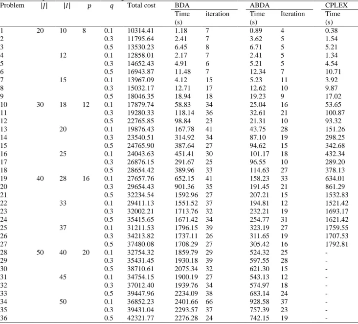
In this section, we present some generated instances to examine the performance of the proposed model and solution approaches. The solution procedures are coded in GAMS23.4 optimization software and all the experiments are performed on an INTEL Core 2 CPU with 2.4 GHz processor and 2 GB of RAM. Note that the termination criteria, “, is considered 108© for solution procedures.We consider the randomly generated, 30-node to 100-node network with a symmetric traveling distance matrix in which the demands are randomly generated at each node. It should be noted that the number of nodes indicates the sum of nodes for candidate facilities’ locations and demand concentrations. The data ranges and obtained results for these generated instances are presented in Tables 1 and 2.In Table 2, BDA and ABDA determine Benders decomposition algorithm and accelerated Benders decomposition algorithm, respectively.
Table 1.Data used in the generated instances
Parameters Values
f< Uª800,2000«
?< Uª40,150«
?< Uª10,100«
Π? max
? `c?<g
Uª0,14
h? Uª1,10«
µ< Uª60,100«
σ< Uª0,10«
< Uª10,40«
?< Uª0,100«
Table 2.Computational results for the generated instances
Problem | | | | Total cost BDA ABDA CPLEX Time
(s)
iteration Time (s)
Iteration Time (s) 1 20 10 8 0.1 10314.41 1.18 7 0.89 4 0.38
2 0.3 11795.64 2.41 7 3.62 5 1.54
3 0.5 13530.23 6.45 8 6.71 5 5.21
4 12 0.1 12858.01 2.17 7 2.41 5 1.34
5 0.3 14652.43 4.91 6 5.21 5 4.54
6 0.5 16943.87 11.48 7 12.34 7 10.71 7 15 0.1 13967.09 4.12 15 5.23 11 3.92 8 0.3 15032.17 12.71 17 12.62 10 9.87 9 0.5 18046.35 18.94 18 19.23 9 17.02 10 30 18 12 0.1 17879.74 58.83 34 25.04 16 53.65 11 0.3 19280.33 118.14 36 32.61 21 100.87 12 0.5 22765.85 98.84 23 21.31 10 93.32 13 20 0.1 19876.43 167.78 41 43.75 28 151.26 14 0.3 23540.51 314.92 34 87.10 19 298.25 15 0.5 24765.90 387.64 27 94.62 15 342.68 16 25 0.1 24043.63 451.41 30 101.17 18 432.34 17 0.3 26876.15 291.67 25 96.55 10 289.20 18 0.5 28654.42 389.96 33 114.63 27 378.13 19 40 28 16 0.1 27657.76 652.15 41 158.23 33 634.01 20 0.3 29654.43 901.36 35 191.45 21 861.29 21 0.5 32234.54 1592.96 27 207.21 15 1532.83 22 33 0.1 29411.13 1551.52 37 194.81 12 1521.42 23 0.3 32002.21 1713.76 32 232.21 19 1693.17 24 0.5 35415.65 1671.42 34 254.77 31 1621.42 25 37 0.1 31211.53 1796.15 39 323.19 27 1759.55 26 0.3 34213.82 1737.11 26 311.65 19 1707.53 27 0.5 37480.08 1708.29 27 305.42 16 1792.81 28 50 40 20 0.1 32754.32 1859.79 29 524.32 25 - 29 0.3 35431.45 1930.18 39 597.55 28 - 30 0.5 38710.61 2075.34 32 621.30 15 - 31 45 0.1 34754.15 1900.19 27 543.13 12 - 32 0.3 37012.40 1939.76 34 574.97 18 - 33 0.5 39447.96 2234.09 38 683.14 24 - 34 50 0.1 36852.23 2401.66 66 928.58 37 - 35 0.3 39431.04 2293.57 37 757.39 23 - 36 0.5 42321.77 2276.28 24 742.15 19 -
Table 2 shows that the total system cost increases as the potential demand for service network increases. For example, the system in 100-node network (e.g.| | = 50 ¬- | | = 50 ) will incur 69.95% much more cost than the one in 30-node network (e.g.| | = 20 ¬- | | = 15 ). Note that this value is obtained by taking the average of total cost over different values. Moreover, the system cost significantly increases as grows. We can see that the system cost under = 0.1 is 23.77% greater than the one under = 0.5 for 30-node network. However, the difference between cost values under different failure probability becomes considerably conspicuous as the number of network nodes increases. The results also confirm the benefit of applying several accelerating methods in the proposed solution procedure such that the accelerated Benders decomposition algorithm becomes significantly more time efficient compared to CPLEX and Benders’ decomposition algorithm. On average, the accelerated Benders decomposition algorithm is 3.91 times faster than Benders decomposition algorithm. Regarding the instances that can be solved by CPLEX, we can conclude that the accelerated benders decomposition algorithm is 5.35 times faster than CPLEX. The convergence plot of the accelerated Benders decomposition algorithm is presented in Figure 1, when | | = 25, | | = 15, = 10 and = 0.3.
Figure 1. The convergence plot of accelerated Benders decomposition algorithm
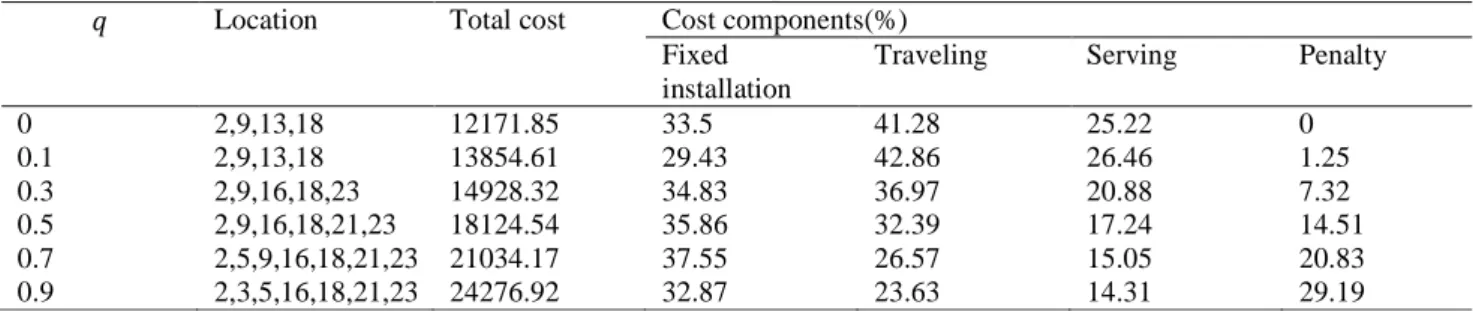
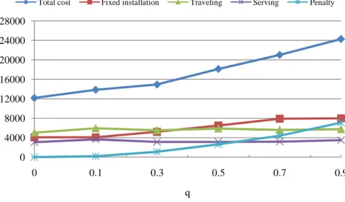
To focus on the impact of failure probability on the system performance, we consider a 40-node network with | | = 25, | | = 15 and = 10. Although some values here may be unrealistic, they can help reveal trends and model behavior. Note that the case = 0 corresponds to the deterministic facility location problem for congested system without the risk of disruptions consideration, and = 1 corresponds to the case where all facilities fail. Table 3 illustrates how the locations and cost components change as failure probability increases. We see that as increases, the total number of constructed facilities somehow increases to hedge against the risk of facility disruptions. We also present the percentage of cost components as the functions of failure probability in Figure 2.
Table 3.Results under different failure probability for 40-node network
Location Total cost Cost components(%) Fixed
installation
Traveling Serving Penalty
0 2,9,13,18 12171.85 33.5 41.28 25.22 0 0.1 2,9,13,18 13854.61 29.43 42.86 26.46 1.25 0.3 2,9,16,18,23 14928.32 34.83 36.97 20.88 7.32 0.5 2,9,16,18,21,23 18124.54 35.86 32.39 17.24 14.51 0.7 2,5,9,16,18,21,23 21034.17 37.55 26.57 15.05 20.83 0.9 2,3,5,16,18,21,23 24276.92 32.87 23.63 14.31 29.19
10000 11000 12000 13000 14000 15000 16000 17000
1 2 3 4 5 6 7 8 9 10 11
L
B
an
d
U
B
v
al
u
e
s
Iteration number
Figure 2.Impact of on the cost components for 40-node network
Figure 3 shows the effect of geographical accessibility on the system costs for a 40-node network with | | = 25, | | = 15 and = 10. When maximum acceptable distance increases, it is expected to install more facilities closer to the demand nodes. However, the fixed installation cost has a relatively steady trend due to the consideration of the maximum number of opened facilities in the model. The constructed facilities can serve demand nodes in the much further locations, and thus, traveling and serving costs grow and penalty cost drops significantly, leading to reduction in the total cost. Therefore, to design an efficient service network, geographical accessibility improvement, maximum number of constructed facilities and cost minimization must be considered concurrently.
Figure 3. Impact of geographical accessibility on the system cost
The effect of on the system costs under different failure probabilities is presented in Figure4. To study more precisely how the failure probability affects the system cost, the values of are considered to be the same for all the candidate locations for facilities.We consider a 40-node network with | | = 25, | | = 15 and = 10. The cost components is illustrated in Figure 5for the case = 0.3. As it can be seen in Figure 4, the penalty cost decreases significantly despite slight increase in investment cost associated with increasing mean service times,
0 4000 8000 12000 16000 20000 24000 28000
0 0.1 0.3 0.5 0.7 0.9
q
Total cost Fixed installation Traveling Serving Penalty
0 3000 6000 9000 12000 15000 18000 21000
20 40 60 80
Maximum acceptable distance
and as a result the total cost decreases. As increases, the existing facilities can provide service for more potential demand and therefore the serving cost has an increasing trend. The traveling cost is relatively insensitive to the changes of . Note that when the mean service times exceed 90, the total cost will increase due to the increase in investment cost. Since the mean service time of each facility can be fully controlled by system designer, it is critical to determine the appropriate value of capacity investment for hedging against the risk of disruptions.
Figure 4.Impact of on the system cost
Figure 5. Impact of on the cost components for = 0.3
6- Conclusions
This paper proposes a reliable location-allocation model to optimize facility location and customer allocations where facilities are subject to the risk of disruptions. Since service facilities are expected to meet random and heavy demands, the congested situations are modeled in service facilities within an M/G/1 queuing system. In order to insure the service quality, a minimum limit reflected in the customers’ expected waiting time is considered in the model. The geographical accessibility of the service network is also considered in terms of the
10000 12000 14000 16000 18000 20000 22000 24000 26000 28000
60 70 80 90 100
µj
q=
0 0.1q= 0.3q= 0.5q=
0 2000 4000 6000 8000 10000 12000 14000 16000 18000 20000
60 70 80 90 100
µj
proximity of a facility to the potential demands. The model determines the minimization of the fixed installation cost as well as expected traveling, serving and penalty costs. A Benders’ decomposition algorithm enhanced by two efficient accelerating methods including valid inequalities and knapsack inequalities is proposed to solve the model. Based on the results, we can conclude that (i) by considering reliability in the location-allocation model, the total number of constructed facilities somehow increases to hedge against the risk of facility disruptions; (ii) the system costs increases as the failure probability increases. Therefore, system designers should put more weight on the worst disruptive situations to obtain more reliable service networks; (iii) since the mean service time plays a significant role in the system cost and performance, it is crucial to determine its appropriate value for hedging against the risk of disruption; (iv)to improve the geographical accessibility, more facilities must be constructed. However, the system cost may increase due to the significant increase in the fixed installation cost. Therefore, to design an efficient service network, geographical accessibility improvement and cost minimization must be considered concurrently; and (vi) the accelerated Benders decomposition algorithm is significantly more time efficient compared to CPLEX and standard Benders decomposition algorithm.
This paper can be extended in several directions. The system disruptions are characterized by the independent and homogenous failure probability in this paper. It would be interesting to model failure probability with heterogeneous and correlated patterns. Considering other queuing systems like M/M/1 and M/M/c will be another direction for future research. The proposed model can also be extended in the situations in which users have incomplete information about the operational status of service facilities.
References.
Aboolian, R., Berman, O., & Drezner, Z. (2009). The multiple server center location problem. Annals of Operations Research, 167(1), 337–352.
Alcaraz, J., Landete, M., Monge, J.F., & Sainz-Pardo, J.L. (2015). Strengthening the reliability fixed-charge location model using clique constraints. Computers &Operations Research, 60, 14–26.
An, Y., Zeng, B., Zhang, Y., & Zhao, L. (2014). Reliable p-median facility location problem: two-stage robust models and algorithms. Transportation Research Part B, 64, 54–72.
Aydin, N., & Murat, A. (2013). A swarm intelligence based sample average approximation algorithm for the capacitated reliable facility location problem. International Journal of Production Economics, 145(1), 173–183. Benders, J.F., 1962. Partitioning procedures for solving mixed-variables programming problems, Numerische Mathematik,4(1), 238–252.
Berman Berman,O., Krass, D., & Menezes, M.B.C. (2007). Facility reliability issues in network p-Median problems: strategic centralization and co-location effects. Operations Research, 55(2), 332–350.
Boffey, B., Galvao, R., & Espejo, L. (2007). A review of congestion models in the location of facilities with immobile servers. European Journal of Operational Research, 178(3), 643–662.
Camargo, R.S.D., Miranda, G., Luna, H.P., 2008. Benders decomposition for the uncapacitated multiple allocation hub location problem.Computers & Operations Research, 35, 1047–1064.
Castillo, I., Ingolfsson, A., Sim, T., 2009. Social Optimal Location of Facilities with Fixed Servers, Stochastic Demand and Congestion, Production and Operations Management, 18, 721 – 736.
Chen, Q., Li, X., & Ouyang, Y. (2011). Joint inventory-location problem under the risk of probabilistic facility disruptions. Transportation Research Part B, 45(7), 991–1003.
Cordeau, J.F., Pasin, F., Solomon, M.M., (2006). An integrated model for logistics network design. Annals of Operations Research, 144 (1), 59–82.
Cui, T., Ouyang, Y., & Shen, Z.M. (2010).Reliable facility location under the risk of disruptions. Operations Research, 58(4), 998–1011.
Drezner, Z. (1987). Heuristic solution methods for two location problems with unreliable facilities. Journal of the Operational Research Society, 38(6), 509–514.
Gross, D., Harris, C.M. Fundamental of Queuing Theory, 3rd ed., Wiley Interscience, New York, 1988.
Hajipour, V., Rahmati, S.H.A., Pasandideh, S.H.R., & Niaki, S.T.A. (2014). A multi-objective harmony search algorithm to optimize multi-server location–allocation problem in congested systems. Computers & Industrial Engineering, 72, 187–197.
Hajipour, V., Zanjirani Farahani, R., & Fattahi, P. (2016). Bi-objective vibration damping optimization for congested location-pricing problem. Computers & Operations Research, 70, 87-100.
Huang, S., Batta, R., & Nagi, R. (2005). Distribution network design: selection and sizing of congested connections. Naval Research Logistics, 52(8), 701–712.
Li, X., & Ouyang, Y. (2010). A continuum approximation approach to reliable facility location design under correlated probabilistic disruptions. Transportation Research Part B, 44(4), 535–548.
Li, X., Ouyang, Y., & Peng, F. (2013a). A supporting station model for reliable infrastructure location design under interdependent disruptions. Transportation Research Part E, 60, 80–93.
Li, Q., Zeng, B., & Savachkin, A. (2013b). Reliable facility location design under disruptions. Computers & Operations Research, 40(4), 901–909.
Lim, M., Daskin, M., Bassamboo, A., & Chopra, S. (2010). A facility reliability problem: formulation, properties, and algorithm. Naval Research Logistics, 57(1), 58–70.
Lim, M.K., Bassamboo, A., Chopra, S., & Daskin, M.S. (2013). Facility location decisions with random disruption and imperfect estimation. Manufacturing & Service Operations Management, 15(2), 239–249.
Marianov,V., & Serra, D. (1998). Probabilistic maximal covering location-allocation models for congested systems. Journal of Regional Science, 38, 401–424.
Marianov, V., &Serra, D. (2001). Hierarchical location-allocation models for congested systems. European Journal of Operational Research, 135(1), 195–208.
Marianov, V. (2003). Location of multiple–server congestible facilities for maximizing expected demand, when services are non-essential. Annals of Operations Research, 123(1), 125–141.
Marianov, V., Rı´os, M., & Icaza, M.J. (2008). Facility location for market capture when users rank facilities by shorter travel and waiting times. European Journal of Operational Research, 191(1), 32–44.
Nosek, R.A., & Wilson, J.P. (2001). Queuing theory and customer satisfaction: a review of terminology, trends, and applications to pharmacy practice. Hospital Pharmacy, 36(3), 275–279.
Peng, P., Snyder, L.V., Liu, Z., & Lim, A. (2011). Design of reliable logistics networks with facility disruptions. Transportation Research Part B, 45(8), 1190–1211.
Pishvaee, M.S., Razmi, J., & Torabi, S.A. (2014). An accelerated Benders decomposition algorithm for sustainable supply chain network design under uncertainty: A case study of medical needle and syringe supply chain. Transportation Research Part E , 67, 14–38.
Preater, J. (2002). Queues in health. Health Care Management Science, 5(4), 283.
Rahmati, S. H. A., Hajipour, V., & Niaki, S. T. A. (2013). A soft-computing Pareto based meta-heuristic algorithm for a multi-objective multi-server facility location problem. Applied Soft Computing, 13(4), 1728– 1740.
Rei, W., Cordeau, J.F., Gendreau, M., Soriano, P., 2009. Accelerating benders decomposition by local branching. INFORMS Journal on Computing, 21(2), 333–345.
ReVelle, C.S., & Eiselt, H.A. (2005).Location analysis: A synthesis and survey. European Journal of Operational Research, 165(1), 1–19.
Revelle, C. S., Eiselt, H. A., & Daskin, M. S. (2008). A bibliography for some fundamental problem categories in discrete location science. European Journal of Operational Research, 184(3), 817–848.
Santoso, T., Ahmed, S., Goetschalckx, M., &Shapiro, A.(2005). A stochastic programming approach for supply chain network design under uncertainty, European Journal of Operational Research, 167(1), 96–115.
Shavandi, H., & Mahlooji, H. (2006). A fuzzy queuing location model with a genetic algorithm for congested systems. Applied Mathematics and Computation, 181(1), 440–456.
Shen, Z., Zhan, R., & Zhang, J. (2011). The reliable facility location problem: formulations, heuristics, and approximation algorithms. INFORMS Journal on Computing, 23(3), 470–482.
Snyder, L.V., & Daskin, M.S. (2005). Reliability models for facility location: the expected failure case. Transportation Science, 39(3), 400–416.
Syam, S.S. (2008). A multiple server location-allocation model for service system design. Computers and Operations Research, 35(7), 2248–2265.
Vatsa, A.K., Jayaswal, S., (2016). A new formulation and Benders decomposition for the multi-period maximal covering facility location problem with server uncertainty. European Journal of Operational Research, 251(2), 404–418.
Verstichel, J., Kinable, J., Causmaecker, P.D., &Berghe, G.V., (2015). A Combinatorial Benders׳ decomposition for the lock scheduling problem. Computers & Operations Research, 54, 117–128.
Wang, Q., Batta, R., &Rump, C. (2002). Algorithms for a facility location problem with stochastic customer demand and immobile servers. Annals of Operations Research, 111(1), 17–34.
Wang, X., & Ouyang, Y. (2013). A continuum approximation approach to competitive facility location design under facility disruption risks. Transportation Research Part B, 50, 90–103.
Weber, Uber den Standort der Industrian, University of Chicago Press, 1909, Translated as (in 1929): Alfred Weber’s Theory of the Location of Industries.
Yun, L., Qin, Y., Fan, H., Ji, C., Li, X., Jia, L., (2015). A reliability model for facility location design under imperfect information. Transportation Research Part B, 81, 596–615.
Zarrinpoor, N., & Seifbarghy, M. (2011). A competitive location model to obtain a specific market share while ranking facilities by shorter travel time. International Journal of Advanced Manufacturing Technology, 55(5), 807–816.
Zhang, Y., Berman, O., &Verter, V. (2009). Incorporating congestion in preventive healthcare facility network design, European Journal of Operational Research, 198(3), 922–935.
Zhang,Y., Berman,O., Verter,V.,2012. The impact of client choice on preventive healthcare facility network design, OR Spectrum, 34, 349–370.
Zhang,Y., Snyder, L.V., Qi, M., Miao, L. (2016). A heterogeneous reliable location model with risk pooling under supply disruptions. Transportation Research Part B, 83, 151–178.