An enhanced robust possibilistic programming approach for forward distribution network design with the aim of establishing social justice: A real-world application

(1)

76

An enhanced robust possibilistic programming approach for

forward distribution network design with the aim of establishing

social justice: A real-world application

Mohammad Hossein Dehghani Sadrabadi

1

, Rouzbeh Ghousi

1*

, Ahmad Makui

1

1_{School of Industrial engineering, Iran University of Science and Technology, Tehran, Iran} [email protected], [email protected], [email protected]

Abstract

The business environment, especially in the supply chain, is virtually fluctuating and is entangled with a lot of problems. Accordingly, a tailored mechanism should be adopted to deal with these problems. To do so, supply chains must take precautionary measures such as storing products and holding safety stock, etc. Given the importance of storage in supply chains, warehouses and depots should be carefully taken into account and located in such a way that their best performance is warranted. In this regard, this paper addresses a robust Multi-Objective multi-product model to design a distribution system under operational risks and disruption considerations. In the proposed model, the objective functions include minimizing the total distribution system cost, the total environmental impacts caused by supply chain along with minimizing the maximum lost sales in customer zones, while taking into consideration possible complete multiple disruptions in facilities and routes between them. Besides, a ε-constraint method is utilized to convert the Multi-Objective problem to a single objective model. In this paper, a two-stage robust possibilistic programming approach is deployed to cope with the uncertainty and disruption risks in the proposed model. Eventually, a real automotive case study is applied to the proposed model, via which the applicability and performance of the proposed model are endorsed. Results indicate that considering operational and disruption risks in the supply chain using two-stage robust optimization will require high costs but it will lead to economic savings and technical advantages in the long term.

Keywords:

Warehouse, robust optimization, uncertainty, fuzzy logic, disruption, distribution network design.

1- Introduction

A distribution chain is a system, consisting of suppliers, warehouses, depots, distribution centers (DC), retailers, and customers. More precisely, in a distribution system, products are supplied, transported, and delivered to customers to meet specific objectives such as minimizing total distribution cost, total distance traveled, etc. Thus, an efficient distribution network management can remarkably improve the system performance by reducing the total system costs and rectifying competitive conditions in the business environment (Ouhimmou et al, 2019). The distribution system

*Corresponding author

Journal of Industrial and Systems Engineering Vol. 12, No. 4, pp. 76 - 106

(2)

77

design problem predominantly encompasses location-allocation decisions and routing sub-problem. Relevant studies include determining optimal shipping routes from supply nodes to demand nodes so that customers’ demands are fulfilled, and the total distribution costs including inventory, shortages, facilities, and transportation costs are minimized (Abareshi & Zaferanieh, 2019; Diabat et al, 2017).

Nowadays, warehouses have a substantial share of costs in the distribution network. In this manner, supply chain management is interested in investigating the location of this component in the logistics network (Le et al, 2019). Warehouses have a direct effect on operational costs in manufacturing systems and also can impress on demand levels in service chains. Warehouses and depots are one of the most outstanding components and echelons of the distribution network (Reyes et al, 2019). Accordingly, they should be carefully taken into account and located in such a way that their best performance is warranted. Indeed, by optimizing a distribution network design problem, optimal location and allocation decisions can be made for warehouses and depots. Given the fact that the business environment is virtually fluctuating and also is entangled with a lot of difficult conditions, the planning of the distribution will be troublesome and costly for companies. Distribution systems may also confront shortages in such cases (Abdel-Basset et al, 2019). As regards any shortage of products in customer zones eventuates in the dissatisfaction as well as reducing company credit, an expedient program should be adopted to deal with uncertainty and prevent shortages (DuHadway et al, 2019). One of the essential principles of designing an efficient distribution network is to observe environmental aspects and create less pollution in the transportation process, holding, operations, etc. Due to the global warming and the need for environmental conservation, supply chain network design needs to be green to minimize environmental damage in addition to achieving minimum cost (Rad & Nahavandi, 2018).

In accordance with the above-mentioned discussions, some corrective actions have been taken to enhance the performance of the distribution network in this study as follows. Given the significance of product shortage in the distribution network, the shortage variable was defined for customer zones, and also the unit cost of the shortage was considered to be a high deficit to reduce the lost sales. As mentioned before, there is a need to optimize transportation, holding, operational, and establishment processes to reduce air pollution and take into account environmental considerations. To this end, we try to manage the distribution system in a way that minimizes the total environmental impact. This article is also able to establish social justice by minimizing the maximum lost sales in customer zones. a two-stage robust possibilistic programming (TSRPP) approach is employed to cope with operational and disruption risks in the proposed model. Notably, robust optimization fortifies model to determine stable decisions for the investigated supply chain. Also, all possible disruptions risks in the investigated supply chain are considered using discrete and independent scenarios and counteracted by a two-stage modeling approach. It is notable to say that disruptions risks are considered in facilities and routes between them. Lastly, a real-world automotive case study is applied to appraise the applicability and performance of the study framework.

This paper is organized as follows. In section 2, we review pertinent literature on distribution network design, as well as stochastic, robust, and fuzzy programming models. Next, in Section 3, we state the problem and propose MILP mathematical formulation. Section 4 explains the solution method to solve the mathematical model. In section 5, the computational results of the model execution based on a real-world case study are presented. Finally, conclusions are provided, and avenues for further research are suggested in section 6.

2- literature review

In this section, a review of relevant researches in the area of facility location-allocation problems (FLAP) and supply chain network design (SCND) under operational and disruption risks are wisely provided. For a detailed overview of FLAP and distribution network design, please see (Farahani et al, 2013; Klose & Drexl, 2005b; Melo et al, 2009). Jafari et al (2010b) proposed a Multi-Objective model in distribution centers location-allocation problems using fuzzy programming. The relationship between distribution facilities is considered in this study. Klose & Drexl (2005b) introduced a facility location model for designing an efficient distribution system. Facility location-allocation decisions cover the core topics of distribution system design. Barreto et al (2007b) proposed a facility routing problem (LRP) based on a clustering approach. The FLRP includes both facility

(3)

location-78

allocation and vehicle routing decisions simultaneously. In this study, they considered a two-level distribution system design and aimed to determine distribution centers and routes among them. Prins et al (2007b) used a hybrid Lagrangian relaxation algorithm to solve an FLRP. They aimed to minimize distribution system cost along with determining optimal routing decisions. (Chen et al, 2008) aimed to solve an FLP using a combination of the ant colony and Lagrangian relaxation algorithms. Lin (2009b) presented a FLAP considering customer service level concerns under uncertainty using chance constraint programming to minimize total cost and meeting customers’ demands. Vincent et al (2010b) used a heuristic algorithm to determine optimal decisions in an FLRP under capacity considerations. Zarandi et al (2011b) presented a fuzzy capacitated FLRP that includes location-allocation and routing decisions to locate depots among a set of candidate nodes. Notably, a time window is taken into account to ensure customer satisfaction in this study. Küçükdeniz et al (2012b) proposed a fuzzy FLAP under uncertainty using convex optimization. In this study, a combination of clustering and fuzzy programming is utilized to solve the problem. Contardo et al (2013) proposed an FLRP that is solved using an exact cut-and-column algorithm. Nadizadeh & Nasab (2014b) presented an FLRP under uncertainty using a fuzzy programming approach that is solved using heuristic algorithms. In this study, the transportation vehicles and other facilities are under capacity considerations and the supply chain (SC) aims to meet customer’s demands with the lowest risk. (Rahmani & MirHassani, 2014b) proposed a facility location problem that aimed to take optimal strategic and operational decisions to satisfy customer’s demands along with minimizing the total system cost. The presented model is solved using heuristic algorithms. Khalili et al (2015) applied an extended queue theory-based model to locate warehouses with capacity considerations in a fuzzy environment optimally, and the study mainly aims to minimize the total cost. Diabat (2016b) discussed a location inventory problem with exclusive sourcing strategies taking into account capacity considerations. Nadizadeh & Kafash (2019b) presented an FLRP in a fuzzy environment with concurrent specified demands. This study aims to minimize the total distribution costs, including routing, opening, and employing of facilities. Khatami Firouzabadi et al (2019b) proposed a hybrid model to make tactical decisions in a glassware manufacturing company. In this study also some MADM techniques are applied.

The model efforts in the area of SCND under disruption and operational risks have mostly focus on different strategies to weaken the destructive impacts of various threats on the SC. Supply chain management (SCM) must take precautionary measures such as storing products and holding safety stock, multiple sourcing, providing backup facilities to cope with disruption risk, which are considered as SC resilience strategies. Silva & De la Figuera (2007b) discussed SCND using backlogging probabilities. In this study, also queue theory is applied, and the customer’s demands considered as a parameter withinherent risk. The problem was solved using an adaptive metaheuristic algorithm. (Garcia-Herreros et al, 2014) proposed a resilient SC taking into account facilities with disruption risks. the developed model has based on DCs with complete and partial disruption, which are modeled using a two-stage stochastic programming approach. (Fattahi et al, 2017) designed a resilient and responsive SC under uncertainty and disruption, considering customers with high sensitivity to delivery time. They proposed a MILP model that customers demand depends on their adopter facilities and the lead times. (Ghavamifar et al, 2018) presented a competitive and resilient SC under disruption risks. In the proposed model, a Bi-Level Multi-Objective Programming (MOP) approach is applied to design a competitive SC. (Diabat et al, 2019) developed a perishable product SCND taking into account facilities' reliability and disruption risks. They utilized robust optimization and multi-criteria decision making (MCDM) to design a resilient supply chain under disruption considerations. (Zahiri et al, 2017) presented a pharmaceutical SCND under uncertainty and disruption considerations applying environmental and social concerns. They utilized a robust hybrid approach to cope with the operational risks within the specified framework.

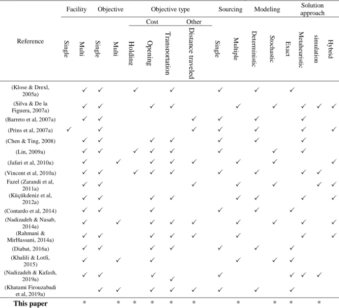
A more detailed classification of the literature on distribution network design is illustrated in Table 1 by considering six characteristics, including type of facilities, number and type of objective functions, sourcing methodology, modeling considerations, and solution approach. Table 1 demonstrates some results as follows. Most facility location problems were costly optimized, and little attention has been paid to other objectives, including minimum total distance, etc. In the reviewed articles, the type of sourcing was often considered single; the mathematical model was mostly

(4)

79

formulated in a deterministic space. Finally, the approach adopted to solve the problem is often metaheuristic.

Table 1. Overview of literature on distribution network design under risk

Reference

Facility Objective Objective type Sourcing Modeling Solution

approach S ing le M ul ti S ing le M ul ti

Cost Other

S ing le M ul tipl e D et er m in is tic S toc ha sti c E xa ct M et ahe u ris tic si m u la tio n H ybr id H ol di ng O pe ni n g T ra ns po rt a tion D is ta n c e tr a v e le d

(Klose & Drexl,

2005a)   _  _  _  _  _  (Silva & De la

Figuera, 2007a)   _   _  _  _    (Barreto et al, 2007a)

          

(Prins et al, 2007a) 

          

(Chen & Ting, 2008)              (Lin, 2009a)              (Jafari et al, 2010a)               (Vincent et al, 2010a)              

Fazel (Zarandi et al,

2011a)             

(Küçükdeniz et al,

2012a)               (Contardo et al, 2014)            

(Nadizadeh & Nasab,

2014a)                (Rahmani &

MirHassani, 2014a)               (Diabat, 2016a)            

(Khalili & Lotfi,

2015)             

(Nadizadeh & Kafash,

2019a)             (Khatami Firouzabadi

et al, 2019a)              

This paper  *  * * * * *  *  * *  *

The proposed research is a Multi-Objective, Stochastic, multiplicative, capacitated, and multiple sourcing FLAP that is solved using an exact methodology. This study takes into account minimizing distribution system costs, total distances traveled by transportation facilities, and establishing social justice in the distribution of end products. In the mathematical model, shortages are calculated in all echelons of the distribution system. We also seek to minimize the maximum shortages occurring in different customer zones to establish social justice in the distribution system. Considering the significant influence of uncertainty and disruption risks on the different facilities, routes among them, product demand, and other parameters, attempts have been made to cope with the operational and disruption risks in the presented framework by developing a two-stage robust possibilistic approach.

The research gaps are extracted as follows. First, the design of a multi-period distribution network, including warehouses, depots, and distribution centers have not been widely discussed in the literature. Second, only a few studies consider disruption in facilities and roots between them simultaneously. Third, only some recent studies take into account disruption and operational risks at the same time. Fourth, most of the available studies do not investigate social justice or social impact in the distribution of products in customer zones. Sixth, only a few studies discussed designing a resilient distribution network that can cope with disruptions at the least cost and damage.

(5)

80

Given the above-mentioned gaps, this paper extends the study area by presenting a novel multi-period, multi-product distribution network design problem, which is a Multi-Objective model to optimize the total distribution network cost, the total environmental impact and maximum lost sale in customer zones. This study takes into account disruption and operational risks by applying a two-stage stochastic programming approach and a robust possibilistic optimization simultaneously. In this study, it is assumed that if a facility or a rout is disrupted, it won’t be accessible and cannot be recovered. The model decisions include locating central warehouses and urban depots as well as determining the amount of product shipped between facilities, the amount of inventory that should be kept in some facilities, and finally, the number of lost sales for different products in each market zones.

2-1- Major contributions in the proposed model

Based on the reviewed papers, we apply some significant contributions to this study. Table 2 illustrates the main contributions considered in the proposed model. First, we take into account simultaneous disruption in facilities, including suppliers cluster, central warehouses, urban depots, distribution centers, customer zones, and routes among them (multiple disruptions). The mentioned contributions are applied in constraint (10-13). It should be noted that the impact of disruption risk on the capacities of each facility is considered with a complete disruption approach, which means a disrupted facility will be Inaccessible. These contributions are considered in constraint (16-25). We also tried to establish social justice in distribution through minimizing the expected maximum lost sale based on disruption scenarios between customer zones, which is applied in term (6). The next contribution enforces coping with the uncertainty using a hybrid two-stage robust possibilistic programming, which is wholly discussed in section 4-1.

Table 2. Major contributions of this study

Contribution The intended purpose

Considering thedisruption in facilities and routes among them simultaneously (multiple

disruptions)

Providing supply chain preparedness to counter disruption risk

Considering complete disruption in different facilities

Taking into account the consequences of supply chain disruption risk

Suggesting Minimizing the maximum lost sales at customer zones as a new objective function

The establishment of social justice in product distribution between different customer zones Coping with uncertainty by applying a hybrid

two-stage robust possibilistic programming

Preventing problem infeasibility and taking into account all possible scenarios for the costs of

establishment and variable costs.

3-Problem statement and mathematical formulation

In this section, we first present the problem description and related assumptions. Next, the problem is formulated using a mixed-integer linear programming (MILP) approach.

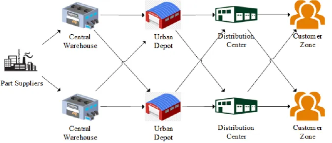
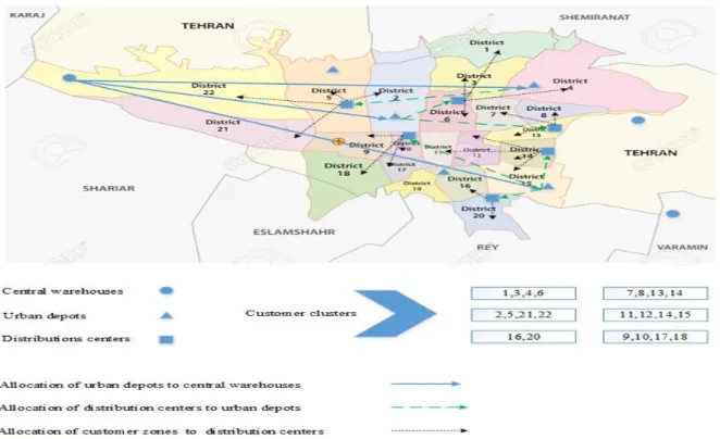
The problem studied in this paper is based on a real-world case. We examine the network design of a forward distribution system that is multi-product, multi-level, multi-period, and multi-stage that is vulnerable to operational and disruption risk. As illustrated in figure 1, the distribution system under investigation consists of different customer zones (CZs), distribution centers (DCs), urban depots (UDs), central warehouses (CWs), and a supplier cluster. The distribution network entails forward flows of products. In the flow of items, central warehouses receive parts from supplier clusters to pack the products and serve urban depots. Authorized products will be shipped from urban depots to the applicant distribution centers. Finally, distribution centers will serve customer zones.

It is assumed that suppliers, central warehouses, urban depots, distribution centers are vulnerable to operational and disruption risks. In other words, disruption risk can completely or partially affect all parameters related to different distribution facilities. To reduce the effects of operational risks, we applied a hybrid robust possibilistic programming model to minimize the total distribution system

(6)

81

cost, comprising costs for lost sales, inventory, transportation, and facility establishment. We also aim to minimize the total environmental impact, and the maximum lost sales occur in customer zones. Here, a two-stage stochastic programming model is utilized to mitigate disruption risks on the route to facilities and in them. The first stage determines the strategic decisions related to the opening of CWs and UDs. The second stage involves determining operational decisions, including allocating CWs to UDs, UDs to DCs, and finally, DCs to CZs. It also includes assessing the number of products transmitted among different nodes of the distribution chain, the inventory amount that should be held in CWs, UDs and DCs considering disruption in facilities and routes. The disruption scenarios investigated in this study are such that if a route or a facility is disrupted, then it would no longer be accessible.

Figure 1 indicates the investigated multi-level distribution system. In the structure of the above-mentioned distribution system, several routes are taken into account between facilities. Notably, only a single route can be selected among the available routes.

Fig 1. Conceptual model of the distribution system

The conceptual questions raised in this study are as follows, which should be answered in the section of results:

 Are distributed products classified independently or considered as family products in the problem?

 How to allocate distribution centers to urban depots to satisfy customer demand?

 Are the selected candidate locations suitable for the establishment of new central warehouses and urban depots?

 Should the problem be investigated in the space of certainty or uncertainty?

 Is there a need to create new central warehouses?

The presented framework determines some strategic and operational decisions as follows:

 Determining number and location of central warehouses and urban depots that can be established among a set of potential locations

 Allocation of customer zones to distribution centers, distribution centers to the urban depots, urban depots to central warehouses to meet customers’ demands

 Determining amounts of transmission between facilities, quantities of inventories and lost sales

 Reducing the cost of opening facilities, holding, transportation, and lost sales

 Establishing justice in supplying parts needed by different customer zones

 Considering the minimum distance traveled between facilities

The following further assumptions regarding the problem formulation should be taken into account:

 Locations are in discrete space.

(7)

82

 Facilities are capacitated in the distribution system to provide service.

 The supply and production capacity of the facilities are different

 In each district, a maximum of one distribution center can exist.

 By increasing cargo volume, transfer costs will increase.

 The cost of opening facilities, the location of the supplier cluster, and customers are known.

 The shortage is allowed in customer zones that are considered as lost sales.

 The customer has the possibility of early delivery of the product, which is subject to holding products.

 The input of the model is known. Therefore, the model is definite and static.

Given the fact that suppliers are obliged to send all of the parts to the central warehouses in the concerned distribution network, so there is no need to define the index of the supplier, and only the total flow of parts shipped from all suppliers to a central warehouse is defined.

3-1- Model formulation

The following sets, parameters, and decision variables are employed to formulate the proposed distribution network design under operational risks and disruption considerations. It should be noted that the beneficiaries of this research are two companies, IKCO and ISACO. Consequently, the model formulation of this research is carried out from their perspective.

3-1-1- Sets and Indices

I Set of potential locations for central warehouses indexed by i 𝑖∈𝐼

J Set of potential locations for urban depots indexed by j j∈J

K Set of different types of product indexed by k 𝑘∈𝐾

L Set of authorized distribution centers indexed by l l∈L

M Set of indexed customer zones indexed by m m∈M

R Set of routes indexed by r r∈R

S Set of disruption scenarios indexed by s s∈S

T Set of time periods indexed by t t∈T

3-1-2-Parameters Technical parameters

max

LD Maximum number of urban depots that can be established

max

CW Maximum number of openable central warehouses that can be established s

jt

HCD Holding capacity of urban depot j in period t under scenario s (m3₎

s lt

HCE

Holding capacity of distribution centers l in period t under scenario s (m3₎

s it

HCW

Holding capacity of central warehouse i in period t under scenario s (m3₎

s kt

SCS

Shipping capacity of product k at supplierclusterin period t under scenarios(ton)

s kit

SCW

Shipping capacity of product _(ton) k at central warehouse i in period t under scenarios

s kjt

SCD Shipping capacity of product k at urban depot j in period t under scenarios(ton)

s klt

SCE

Shipping capacity of product k at distribution center l in period t under scenarios( nto )

s kit

ACW

Receive capacity of product k at central warehouse i in period t under scenarios( ont ) s

kjt

(8)

83 s

klt

ACE

Receive capacity of product k at distribution center l in period t under scenarios(ton)

s kmt

DEC

Demand of product k at customer zone m in period t under scenarios(ton) Vk The volume occupied by a product k (m3/ton)

d

ijr Distance between central warehouse i and urban depot j by route r(Km)

d

jlr Distance between urban depot j and distribution center l by route r(Km)

d

lmr Distance between distribution center l and customer zone m by route r(Km) s

t

 A binary parameter, equal to 1 if supplier clusteris disrupted in period t under scenario ; s

0, otherwise.

s it

 A binary parameter, equal to 1 if central warehouse i is disrupted in period t under s

scenario ; 0, otherwise.

s jt

 A binary parameter, equal to 1 if urban depot j is disrupted in period t under scenario ; s 0, otherwise.

s lt

 A binary parameter, equal to 1 if distribution center l is disrupted in period t under s

scenario ; 0, otherwise.

s irt

 A binary parameter, equal to 1 if route r between supplier cluster and central warehouse i is disrupted in period t under scenario ; 0, otherwise. s

s ijrt

 A binary parameter, equal to 1 if route r between central warehouse i andurban depot j

is disrupted in period t under scenario ; 0, otherwise. s s

jlrt

 A binary parameter, equal to 1 if route r between urban depot j and distribution center l

is disrupted in period t under scenario ; 0, otherwise. s

s lmrt

 A binary parameter, equal to 1 if route r between distribution center l and customer zone

m is disrupted in period t under scenario ; 0, otherwise. s

Economic parameters

j

FOD _{Fixed cost of opening urban depot}_{j (million rials)}

i

FOW Fixed cost of opening central warehouse m (million rials) s

kjt

HOD Unit cost of holding product k at urban depot j in period t under scenario s (million rials / ton)

s klt

HOE Unit cost of holding product k at distribution center l in period t under scenario s

(million rials / ton) s

kit

HOW Unit cost of holding product _s k at central warehouse in period i t under scenario

(million rial / ton) s

kijrt

TWD Unit transportation cost of product k from central warehouse ti o urban depot j by route r in period tunder scenarios (million rials / ton.km)

s kjlrt

TDE Unit transportation cost of product k from urban depot j to distribution center l by route r in period t under scenarios (million rials / ton.km)

s klmrt

TEC

Unit transportation cost of product _route_r_{in period}_t _{under scenario}_s_{(million rials / ton.km)}k from distribution center tl o customer zone m by

s kirt

TSW

Unit transportation cost of product _route_r_{in period}_t_{under scenario}_sk_{(million rials / ton.km)} from supplier cluster to central warehouse by i

s kmt

SHCE

Unit cost of lost sales for product _{(million rials / ton)} k at customer zone m in period t under scenario s

Environmental parameters

EOD j Unit environmental impact associated with establishing urban depot j (amount / ton) EOWi Unit environmental impact associated with establishing central warehouse _ton) i (amount /

s kit

(9)

84 s

kjt

EHD Unit environmental impact of holding product k at urban depot j in period t under scenario s (amount / ton)

s klt

EHE

Unit environmental impact of holding product _{under scenario}_s_{(amount / ton)} k at distribution center l in period t

s kijrt

ETWD Unit environmental impact of shipping product k from central warehouse i to urban depot j by route r in period tunder scenarios (million rial / ton.km)

s kjlrt

ETDE Unit environmental impact of shipping product _{center l} k from urban depot j to distribution by route r in period t under scenarios (million rial / ton.km)

s klmrt

ETEC

Unit environmental impact of shipping product _{customer zone m}_{by route}_r_{in period}_t _{under scenario}k _s_{(million rial / ton.km)}from distribution center l to

s kirt

ETSW

Unit environmental impact of shipping product _warehouse_{by route}_i _r_{in period}_t_{under scenario}k_s_{(million rial / ton.km)}from supplier cluster to central

3-1-3- Decision variables

s klmrt

FEC

Quantity of product k shipped from distribution center l to customer zone m by route r

in period t under scenarios (ton)

s kijrt

FWD Quantity of product k shipped from central warehouse i to urban depot j by route r in period t under scenarios (ton)

s kjlrt

FDE Quantity of product k shipped from urban depot j to distribution center l by route r in period t under scenarios (ton)

s kirt

FSW

Quantity of product k shipped from supplier to central warehouse i by route r in period t

s under scenario (ton)

s kit

IW

Inventory of product k at central warehouse i in period t under scenarios (ton) s

kjt

ID Inventory of product k at urban depot j in period t under scenarios (ton)

s klt

IE

Inventory of product k at distribution center l in period t under scenarios (ton)

s kmt

SLC

Lost sale of product k at customer zone m in period t under scenarios (ton) j

OD A binary variable equal to 1 if urban depot j is established; 0, otherwise.

i

OW

A binary variable equal to 1 if central warehouse i is established; 0, otherwise.

s ijrt

WD A binary variable equal to 1 if urban depot j is allocated to central warehouse i by

route r in period t under scenario ; 0, otherwise. s s

jlrt

DE A binary variable equal to 1 if distribution center l is allocated to urban depot j by route

r in period t underscenario ; 0, otherwise. s

s lmrt

EC

A binary variable equal to 1 if customer zone m is allocated to distribution center l by

route r in period t under scenario ; 0, otherwise. s

After applying the two-stage modeling procedure (Sabet et al, 2019) to our problem, the mathematical model is then as follows:

3-1-4- Objective functions Total cost

The objective function (1) guarantees the minimization of the total distribution costs, including transportation, establishment, holding, and shortage costs.

(10)

85

( 1 )

( s s s s

j j i i s kjt kjt klt klt j J i I s S k K j J t T k K l L t T

s s s s s s

kit kit kirt kirt kijrt kijrt ijr k K i I t T k K i I r R t T k K i I j J r R t T

s klmrt

Min TC FOD OD FOW OW HOD ID HOE IE

HOW IW TSW FSW TWD FWD d

TEC                              



  







)

s s s

klmrt lmr kjlrt kjlrt jlr k K l L m M r R t T k K j J l L r R t T

s s kmt kmt k K m M t T

FEC d TDE FDE d

SHCE SLC               

  



  

Total environmental impact

The total environmental impact, including transportation (TTEs), establishment (TOE), and holding (THEs) impacts are defined as the second objective function by terms (2-5).

( 2 )





s s s

s S

MinTEI TOE TTE THE



 



 

( 3 )

s s s s

o kirt kirt kijrt kijrt ij

k K i I r R t T k K i I j J r R t T

s s s s

klmrt klmrt lm kjlrt kjlrt jl

k K l L m M r R t T k K j J l L r R t T

TTE ETSW FSW ETWD FWD d

ETEC FEC d ETDE FDE d

                      

   

    

( 4 )

s s s s s s

kjt kjt klt klt kit kit

k K j J t T k K l L t T k K i I t T

THEo EHOD ID EHOE IE EHOW IW

        



  



  



  

( 5 )

j j i i

j J i I

TOE EOD OD EOW OW

 









Establishing social justice

One of the most essential considerations in distribution network design is to ensure fairness in the distribution of products to customer zones. To aim this, we tried to minimize the expected maximum lost sale based on disruption scenarios between customer zones and establish social justice through the non-linear term (6). This objective function is a nonlinear term, and it should be linearized to reduce problem complexity.

( 6 )

s

s kmt

m k K s S t T

SLC MinMax        3-1-5- Constraints ( 7 ) l L , s S

   

1

s jlrt r R

DE







( 8 ) ,

j J s S

   

1

s ijrt r R

WD







( 9 ) ,

m M s S

   

1

s lmrt r R

EC







( 10 ) , ,

j J l L s S

     



1



1



1



s s s s

jlrt j jt lt jlrt

(11)

86

( 11 )

, ,

i I j J s S

     



1



1



1



s s s s

ijrt i it jt ijrt

WD OW 











( 12 )

, ,

i I j J s S

     



1



1



1



s s s s

ijrt j it jt ijrt

WD OD 











( 13 )

, ,

i I j J s S

     



1



1



s s s

lmrt lt lmrt

EC  







( 14 ) max j j J OD LD  



( 15 ) max i i I

OW

CW







( 16 ) , ,

k K t T s S

     



1



s s

kirt kt t

i I r R

FSW SCS     



( 17 ) , , ,

k K i I t T s S

     



1



s s

kijrt kit it i

j J r R

FWD SCW OW

    



( 18 ) , , ,

k K j J t T s S

       



1



s s

kjlrt kjt jt j

l L r R

FDE SCD OD

    



( 19 )

,

k

K

l

L

t T

s

S

       



1



s s

klmrt klt lt

m M r R

FEC

SCE

 



 

 

( 20 ) , , ,

k K i I t T s S

     



1



s s

kirt kit it i

r R

FSW ACW OW

   



( 21 ) , , ,

k K j J t T s S

       



1



s s

kijrt kjt jt j

i I r R

FWD ACD OD

    



( 22 )

,

k

K

l

L

t T

s

S

       



1



s s

kjlrt klt lt

l L r R

FDE

ACE

 



 



( 23 ) , ,

j J t T s S      



1



s s

k kjt jt jt j

k K

V ID HCD OD

   



( 24 ) , ,

i I t T s S      



1



s s

k kit it it i

k K

V IW HCW OW



  

(12)

87

( 25 )

, ,

l L t T s S      



1



s s

k klt lt lt

k K

V IE HCE

   



( 26 ) , ,

j    J l L s S

s s

kjlrt jl

k K r R t T

FDE

BM DE

  





( 27 ) , ,

i    I j J s S

s s

kijrt ij

k K r R t T

FWD

BM WD

  





( 28 ) i I   s kirt i

k K r R t T s S

FSW

BM OW

   





( 29 ) , ,

l L m M s S

     

s s

klmrt lm

k K r R t T

FEC BM EC

   



( 30 )

,

i I

j J

s S

     

s s

kijrt ij

k K r R t T

FWD

BM WD

  





( 31 ) , ,

j J l L s S

     

s s

kjlrt jl

k K r R t T

FDE

BM DE

  





( 32 )

,

k

K

m M t T

s S

   

  

s s s

klmrt kmt kmt

l L r R

FEC

SLC

DEC

 







( 33 )

,

k

K

l

L

t T

s S

   

1

s s s s

klt klt kjlrt klmrt

j J r R m M r R

IE IE _ FDE FEC

     





 

( 34 )

,

k

K

j

J t T

s

S

   

  

1

s s s s

kjt kjt kijrt kjlrt

i I r R l L r R

ID

_

FWD

FDE

   











( 35 )

,

, ,

,

k

  

K

i

I

t

  

T

s

S

1

s s s s

kit kit kirt kijrt

r R j J r R

IW IW _ FSW FWD

    







( 36 ) , , , , , ,

i I j J k K l L m M s S t T

       

     

, , , , , , ,

0

s s s s s s s

klmrt kijrt kjlrt kirt kit kjt klt s

kmt

FEC FWD FDE FSW IW ID IE SLC  ( 37 ) , , , , , ,

i I j J l L m M r R s S t T

         

   

 

, , s , s , s 0,1

j i ijrt jlrt lmrt OD OW WD DE EC 

(13)

88

Constraints (7-9) ensure that between supplier cluster and each central warehouse, each central warehouse and urban depot and finally each urban depot and distribution center, one root is allocated. Constraint (10) enforces that if an existing distribution center is allocated to an opened urban depot, facilities and routes between them are not disrupted. Constraints (11-13) state the same condition as the constraint (10) between echelons supplier cluster and central warehouse, central warehouse and urban depot, distribution center, and customer zone. Constraints (14-15) stipulate the maximum number of urban depots and central warehouses that can be established. Constraints (16-19) provide that the transportation amounts must not exceed the shipping or supply capacity of supplier cluster, central warehouses, urban depots, and distribution centers considering complete disruption risk in facilities. Constraints (20-22) stipulate that the number of products that are shipped to a facility must not exceed the receiving capacity of that facility considering complete disruption risk in facilities. Constraints (23-25) provide that Inventory amounts kept by a facility must not exceed the holding capacity of that facility considering complete disruption risk in facilities. Constraints (26-31) guarantee that products cannot be shipped from a facility to another facility to which it is not assigned. Constraint (32) provides demand satisfaction for customer zones. Constraints (33-35) are inventory balance equations for central warehouses, urban depots, and distribution centers. Constraints (36-37) provide binary and non-negativity restrictions on the decision variables.

4- Solution approach

The optimization model proposed in the previous section is entangled with a series of the problems, including (1) the third objective function is taken into account a non-linear term and should be converted into a linear form, (2) Some parameters in the proposed model are affected by uncertainty, for which an appropriate method is needed to be employed to cope with such operational risks, (3) the proposed model encompasses two objective functions. Accordingly, we should exploit a Multi-Objective programming (MOP) method to solve the model.

The following actions took place to tackle the above-mentioned problems:

 The maxi-min objective function as a non-linear term has been converted into a linear form by applying an appropriate procedure

 A two-stage robust possibilistic programming model is utilized to capture the operational risks

 To convert the proposed Multi-Objective model into single-objective one, ɛ-constraint method is deployed.

4-1- linearization approach

As mentioned before, the objective function (3) is considered as a non-linear term that destroys the linearity condition of the proposed model. The nonlinear term can be converted into the linear one by applying the constraints (38-39) as follows:

(38) Min SV

(39)

m

M

 

s

s kmt

k K s S t T

SLC SV

  

 

  

4-2- The implementation of MOP

4-2-1- ɛ-constraintmethod

MOP enables Multi-Objective problems to be optimized over a feasible region. Different approaches are proposed to transform a Multi-Objective problem into single-objective such as no-preference methods, priori methods, posteriori methods, interactive methods, etc. In this study, the ɛ -constraint method is employed to convert the Multi-Objective model into a single objective formulation.

An exclusive benefit of applying the ɛ-constraint method in Multi-Objective problems is that by restraining efficient solutions, Pareto frontier can be easily obtained. ɛ-constraint is a powerful method with tangible success in MOP, notably in SCND problems (Olivares-Benitez et al, 2013). In multi-objective problems, multi-objectives are either minimization or maximization. Solving multi-multi-objective problems using ɛ constraint includes a methodology as follows: First, we must determine the objective

(14)

89

function with the highest priority and consider it as the main objective, and then we must define the acceptable ɛ bounds for the remaining objectives. In fact, in the ɛ-constraint method, one objective function is optimized while ɛ bounds restrict the other objective functions. Consequently, we will define a new single objective problem (Dehghani et al, 2018a). Lower ɛ bounds are considered for the objective functions of maximizing, and upper ɛ bounds are provided for the minimization objective functions. we apply mathematical expressions as follows:

Suppose that a Multi-Objective problem is generally defined as follows:

1

, ...,

,... ,

1

, ...,

. :

k j

j n

Min f

f

Max f

f

S t

X





(40)

 represents the feasible region that can be defined by equality and, or inequality constraints. If the objective function fk is identified as the highest priority objective in Multi-Objective problem and the vector ɛ is defined as ɛ bounds for other objective functions. The Multi-Objective problem is solved using the ɛ-constraint method as follows:

1 1 1 1

,..., ,...., ,..., k

k k

k k j j

j j n n

Min f

f f

X

 

   

   

   



(41)

Where the vector of upper and lower ɛ bounds,





( ,

 

1 2

,...,



n

)

, Specifies the upper limit

for minimization objective functions and the lower limit for objective functions of maximizing. It should be noted that by altering the epsilon bound vector along the Pareto frontier and making a new optimization problem for each new vector, the Pareto optimal set can be achieved.

Determining upper and lower ɛ bounds

At each iteration of the ɛ-constraint method, lower and upper ɛ bounds are determined as follows. Suppose that objective function fk has the highest priority for the decision-maker. First, we solve a single objective problem based on fk as objective function and technical constraints as follows

:

k

Min f

X

 

(42)

Consider vector X*_{as an optimal solution for the above-mentioned problem, so Z}nadir_{will be} obtained for both objectives of maximizing and minimizing as follows:

*

( )

Nadir

i i

Z  f X  i 1, 2,...,k1,k1,...,n (43)

After that, we will optimize objective functions independently except fk to determine the optimal objective functions vector Z*_{as follows:}

* *

( )

i i

Z



f

x

 i 1, 2,...,k1,k1,...,n (44)

Upper ɛ bounds vector,

  

( , ,...,1 2



k1), indicates the maximum value that each objective of minimizing can have. Suppose that the problem is executed in n iterations, upper ɛ bounds are determined in each iteration r as follows:

(15)

90





* nadir *

i i i i

r

Z Z Z

n

     i 1,2,...,k1 (45)

Lower ɛ bounds vector,

  

( k1, ,..., )2



n , specifies the minimum value that each objective of maximizing can have. Suppose we have n iterations; lower ɛ bounds are determined in each iteration r as follows

:



*



nadir nadir

i i i i

r

Z Z Z

n

      i k 1,...,n (46)

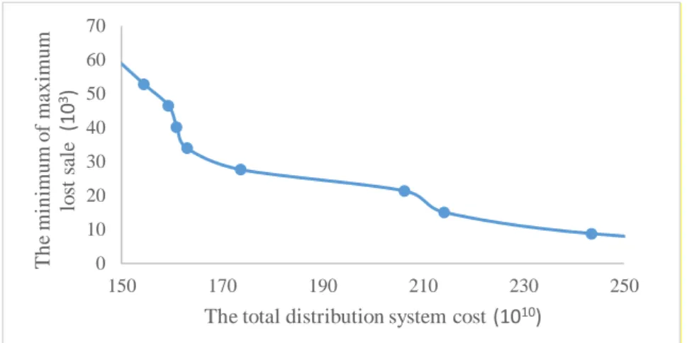
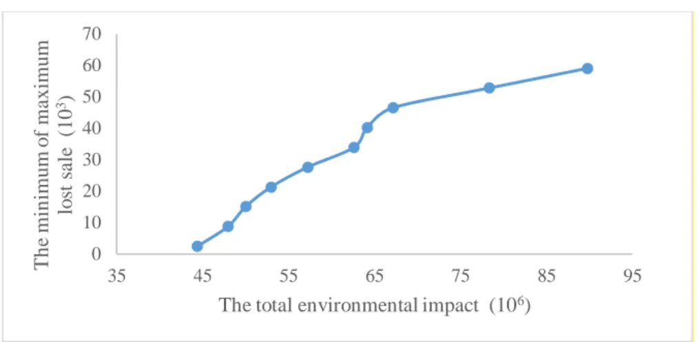
As mentioned before, the Pareto optimal set can be achieved by altering the ɛ bounds vector along the Pareto frontier. It is noteworthy that the generation of points on the Pareto frontier is illustrated in the section of results.

4-3- Robust optimization method

In this section, we apply a robust optimization approach to extend the proposed deterministic model in a robust formulation. Robust optimization techniques are efficient approaches to cope with different operational risks, especially in situations of inappropriate historical data or lack of knowledge to estimate the probability distributions of uncertain parameters.

In this study, a robust possibilistic method is provided to cope with the uncertainty of variable costs, fixed opening costs, demands, capacities, and other parameters of distribution network design model that are faced to uncertainty. For this purpose, we used the research carried out in 2012 by Pishvae et.al the robust possibilistic applied in this study, was based on an optimistic approach, so the objective function was significantly increased, but instead, maximum lost sales of products at customer zones was decreased. It should be noted that robustness was applied throughout the constraints, but only the most critical objective function, or in other words, minimization of the total distribution system costs (Dehghani et al, 2018b; Pishvaee et al, 2012b; Zokaee et al, 2017).

To work more convenient, the deterministic distribution network design problem studied in this paper (excluding second and third objective function) can be compactly formulated as follows:

 

1 1 2 2

. :

0,1 0

Min Z FY CX

S t

A X D A X D Y

B X S B X S Y

C X P C X P Y

Y X

 

 

 

 

(47)

Where the vectors F, C, D1, D2, S1, S2, P1, and P2 indicate the fixed opening, variable transmission, holding and shortage costs, requirements for available facilities like distribution centers and customer zones, requirements for facilities that need opening, holding capacities for available facilities, holding capacities for facilities that require opening, shipping capacities for available facilities, shipping capacities for facilities that require opening, respectively. The matrices A1, A2, B1, B2, C1, and C2, are technical coefficient matrices of constraints. Additional vector Y and X define the binary opening variable and continuous inventory and flow variables, respectively. It should be noted that to apply the robust optimization to the proposed model, it is first necessary to convert the Multi-Objective problem to a single-objective problem using the ɛ-constraint method, then the robust optimization process can be executed.

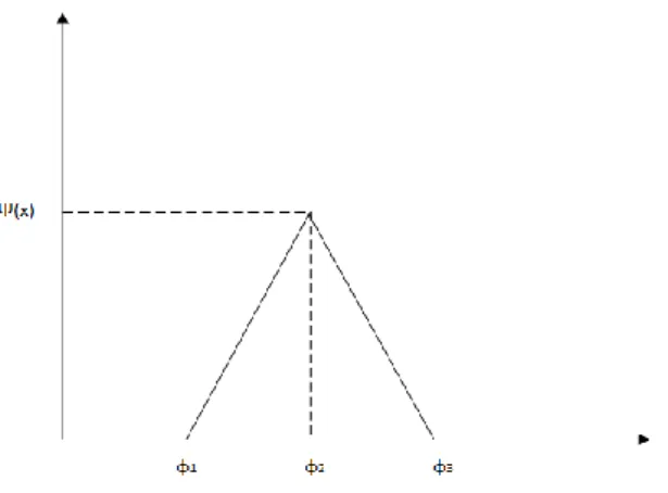
Now consider vectors F, C, and technical coefficient matrices D1, D2, S1, S2, P1, P2 that represent the capacity and demand of facilities are the uncertain parameters in the formulation of the deterministic model. The expected value operator has been used to model the first objective function and the necessity measure to cope with chance constraints, including uncertain parameters that can be defined by triangular possibility distribution or triangular fuzzy number. Figure 2 illustrates that a membership function defines a triangular fuzzy number.

(16)

91

Fig 2. The triangular possibility distribution of fuzzy parameter



Based on the above-mentioned discussions, the FLAP chance constraint programming model can be stated for an optimistic formulation as follows:

























 

1 1 2 2

. :

0,1 0

Min Z E F Y E C X S t

Pos A X D Pos A X D Y

Pos B X S Pos B X S Y

Pos C X P Pos C X P Y

Y X      _{ }  _{ }                     (48)

The equivalent crisp model of the above formulation can be stated as follows:

 

(1) ( 2) (3) (1) ( 2) (3)

(1) ( 2) (1) ( 2)

1 1 1 2 2 2

(3) (1) (3) (1)

1 1 1 2 2 2

(3) (1) (3) (1)

1 1 1 2 2 2

[ ]

3 3

. :

(1 ) ( (1 ) )

0,1 0

f f f c c c

Min E Z Y X

S t

A x D D A x D D y

B X S S B X S S y

C X P P C X P P y

Y X         _ _ _ _                                     (49)

In formulation (49), it is assumed that chance constraints should be satisfied with the confidence level that are parameters, and DM should determine these two parameters greater than 0.5, but determining confidence levels cause lowering mathematical accuracy.

Based on (Pishvaee et al, 2012a), the most accurate mathematical model for robust possibilistic FLAP can be formulated as follows:

 

(3) (1) (2) (3) (1) (2)

max min 1 1 1 1 2 2 2 2

(3) (1) (1) (3) (1) (1) (3) (1) (1)

1 1 1 1 2 2 2 2 1 1 1 1

(3) (1) (1)

2 2 2 2

( ) (1 ) (1 )

(1 ) (1 ) (1 )

(1 )

Min E Z Z Z D D D D D D Y

S S S S S S Y P P P

P P P

       _    _ _    _        _    _ _    _  _    _    _    _                   

 

(1) (2) (1) (2)

1 1 1 2 2 2

(3) (1) (3) (1)

1 1 1 2 2 2

(3) (1) (3) (1)

1 1 1 2 2 2

. :

(1 ) ( (1 ) )

0,1 , 0 , 0.5 , 1

Y

S t

A x D D A x D D y

B X S S B X S S y

C X P P C X P P y

Y X                                     (50)

(17)

92

In formulation (50), the first term in the objective function represents the expected value of z that results in the minimization of the expected total distribution system cost. The second term,

max min

(Z Z )

 , illustrates the difference between the two extreme possible values of the objective function in which zmax and zmin can be defined as follows:

max (3) (3)

min (1) (1)

Z f y c x Z f y c x

 

  (51)



indicates the importance weight of this difference that is determined by DM. The third term,

(2) (1) (2) 1D1  D1  (1 )D1 

   , considers the confidence level of each chanceconstraints in which 1 is the unit penalty of the possible infeasibility of each constraint including an imprecise parameter (D1) and the term ( 2) (1) ( 2)

1 1 (1 ) 1

D D D

    

    indicates the difference between the worst-case value of an uncertain parameter and the value that is used in chance constraint programming. Other terms and parameters in objective function can be defined as the third term, but in some terms that are related to facilities that require opening, an opening variable y and Confidence level variables  or  are multiplied.

As it can be seen in the formulation (50), when parameters are assumed to be imprecise, the linearity of the chance constraints and the first objective function is destroyed in the proposed robust possibilistic programming model. The non-linear terms can be converted into the linear by defining some new auxiliary variables and adding several constraints to the primary model. To reduce the complexity of the non-linear problem and also easier to solve the model by exact algorithm, let w1and

w2 be auxiliary variables(vectors) that are defined as