249
Solving a bi-objective multi-commodity two-echelon capacitated
location routing problem
Masoud Rabbani
1*, Seyed Mohammad Zenouzzadeh
2, Hamed Farrokhi-Asl
11 School of Industrial and Systems Engineering, College of Engineering, University of Tehran,
Tehran, Iran
2 School of Industrial Engineering, Iran University of Science and Technology, Tehran, Iran
[email protected], [email protected], [email protected]
Abstract
Planning the freight flow from the plants to the customer zones is one of the most challenging problems in the field of supply chain management. Because of many traffic regulations, oversize/overweight vehicles often are not permitted to enter city boundaries. Therefore, intermediate facilities (city distribution centers) play a very important role in distribution networks. Accordingly, in this paper, transportation of goods from the plants to the customers is considered an integrated process containing two phases, namely, transportation from plant to distribution centers and distribution from city distribution centers to customers using small and environmentally-friendly vehicles. The Transportation Location Routing Problem (TLRP) studied can be considered as an extension of the two-echelon location routing problem. Minimizing the operational costs, and the workload balancing of the heterogeneous fleet in the distribution phase are considered as the two objective functions. A mixed integer programming (MIP) model, as well as two solution approaches, based on Multi-objective Particle Swarm Optimization Algorithm, and Non-dominated Sorting Genetic Algorithm, is presented for the problem. In order to illustrate the efficacy of the proposed methods, they have been implemented on test problems of different sizes. The results show the methods are able to produce efficient solutions in a reasonable amount of time.
Keywords: Location routing problem, multi commodity, metaheuristic algorithms, multi-objective optimization
1-Introduction
In Supply Chain Management (SCM), distribution system design comprises the operations and decisions regarding how to deliver the final products from the plants to the customers. City administrations impose regulations on oversize/overweight vehicles to reduce adverse impacts such as traffic congestion and air pollution on the urban areas. These restrictions make direct delivery of products from plants to customers either uneconomical or even infeasible. Considering these constraints, logistic operators have come up with a solution: City Distribution Centers (CDCs).
*Corresponding author
ISSN: 1735-8272, Copyright c 2019 JISE. All rights reserved Journal of Industrial and Systems Engineering
Vol. 12, No. 3, pp. 249- 268 Summer (July) 2019
250
CDCs are warehouses, often located outside city boundaries, to which the products are transported from plants, to be distributed to retailers, wholesalers or directly to customers. Heavy vehicles unload their cargo to CDCs. The loads are then categorized and assigned to small and environmentally-friendly vehicles to be delivered within the city limits (Crainic et al., 2007). With the advent of CDCs, came the strategic decision of location selection for the CDCs as well as routing decisions from CDCs to clients. Also, it was necessary that the delivery of products from plants to CDCs be optimized. Hence, the planning is divided into three stages: (1) CDC location allocation, (2) distribution (routing) planning, and (3) Routing/transportation of goods from plants to CDCs.
Some research studies, such as Chen (2001), Aikens (1985) and Lan and Li (2010) viewed the location problem as an isolated strategic decision-making process. Some others, on the other hand, taking into account routing aspects, introduced Location Routing Problem (LRP). According to Hassanzadeh et al., (2009), studies such as Or and Pierskalla (1979), Jacobsen and Madsen (1980) and Laporte and Nobert (1981) are among the pioneers in introduction and extension of LRP as a combined problem. LRP models can be considered a combination of Facility Location Problems (FLPs) and Vehicle Routing Problems (VRPs) (For further information about LRP see Drexl and Schneider (2015), Nagy and Salhi (2007)). These approaches, however, still ignore the interconnection between the decisions related to the transportation of goods from plants to distribution centers and the decisions regarding the distribution phase.
To overcome this shortcoming, Gonzalez-Feliu et al. (2008) introduced a new family of VRPs, namely, Multi-echelon VRP (2E-VRP). The underlying idea of multiple-echelon VRPs is that the products are not delivered directly to the customers; instead, in an NE-VRP, customers are served via N legs in an N-stage distribution network. In their work, Gonzalez-Feliu et al. (2008) propose an MIP formulation of 2E-VRP as well as some valid inequalities for the problem. Gonzalez-Feliu et al. (2008) utilized a similar formulation and presented some other valid inequalities and two metaheuristics as well. Crainic et al. (2008) presented several meta-heuristics based on separating the two stages of the problem. Some valid inequalities based on TSP and CVRP, the network flow formulation and the connectivity of the transportation system are presented by Perboli and Tadei (2010). Despite the valuable efforts devoted to the field of NE-VRPs, in terms of proposing new formulations, valid inequalities and solution methods, they still neglected to consider the decisions regarding the location of CDCs.
In fact, the decisions related to the location of CDCs, transportation of goods from plants to CDCs and vehicle routing are highly interrelated. It has been proved that considering these problems separately, results in sub-optimal solutions (Farham et al., 2018; Rabbani et al., 2018). Therefore, an integrated approach is required to tackle these problems in a single framework. As a result, a new class of LRPs was introduced: multiple-echelon LRP. This class of problems, in the recent decade, has received tremendous attention from researchers. The problem consists of two or more integrated decision layers. In each layer, some facilities should be located. The demand of a given open depot in a given intermediate level is considered equal to the summation of the demands of the nodes associated with and are planned to be served by the given facility. Solving a Bi-objective Multi-commodity Two-echelon Capacitated Location Routing Problem 3 Product delivery in each layer (stage) may be either conducted using routing or direct transportation. In the former setup, the vehicle may serve several nodes, whereas, in the latter, it serves just one node.
The problem of NE-LRP was formally introduced by Ambrosino and Scutella (2005), for the first time. The authors investigated several realistic scenarios, and for each scenario, proposed two different mathematical programming approaches. Boccia et al., (2010) developed a Tabu Search heuristic, which decomposes the problem into four sub-problems. The solutions to the sub-problems are aggregated afterwards to provide a global solution to the problem. Nguyen et al. (2010) proposed a hybrid method to solve 2E-LRP. The method is a hybridization of a Greedy Randomized Adaptive Search (GRASP) and an evolutionary/iterated local search. A new four-index MIP model was presented by Nikbakhsh and Zegordi (2010). In their proposed model, the authors consider soft time window constraints. They also propose a heuristic algorithm and a lower bound for the problem. Crainic et al. (2011) implemented a tabu search meta-heuristic to solve a two-echelon location routing problem. The proposed method is based on the decomposition of the problem into two LRPs, one for each echelon. Afterward, each LRP is decomposed into a capacitated facility location problem (CFLP) and a multi-depot vehicle routing problem (MDVRP). Therefore, four sub-problems are
251
generated, the solutions of which are combined using an iterative-nested approach. In another work (Punyim et el., 2018), an iterative-nested tabu search heuristic was applied to solve a location-inventory on a two-level supply chain in which one plant provides a one type of product to a set of facilities which supplies a set of customers with stochastic demands. They tested the performance of the algorithm with 100 possible parameter combinations on test problems to determine the best parameter combination. Due to the similarities between 2E-LRP and the classical form of LRP, a previously successful solution method based on Variable Neighborhood Search (VNS) is utilized by Schwengerer et al. (2012) to tackle 2E-LRP. Another hybrid solution method made up of a Genetic Algorithm (GA) and a Simulated Annealing Algorithm (SA) was applied by Dalfard et al. (2013). Rahmani et al. (2013) presented a new extension of 2E-LRPs: 2E-LRP with Multi-products, Pickup and Delivery (2E-LRP-MPPD). Also, a mathematical formulation, as well as a heuristic solution approach for the problem was proposed. The authors, in a later study, Rahmani et al. (2015) presented two local search methods to solve the problem mentioned above. Another similar extension of the problem was introduced by Demircan-Yildiz et al. (2016). The paper addressed the so-called two-echelon location routing problem with simultaneous pickup and delivery (2E-LRPSPD) and proposed two MIP formulations for the problem. The authors also borrowed a family of valid inequalities from the literature to enhance the performance of the proposed formulations.
In a research conducted by Dakkanci et al. (2019), the authors tackled a two-echelon location-routing problem aiming to optimize economic and environmental objectives. A hybrid method of Multi-objective Particle Swarm Optimization (MOPSO), initially developed by Coello Coello (2002), and Adapted Multi-objective Variable Neighborhood Search (AMOVNS) was used to solve the problem. The multi-objective format of the problem was also studied by Martínez-Salazar et al. (2014). The two objective functions were (i) minimization of total costs including CDCs’ opening costs (fixed costs) and routing costs (variable costs) and (ii) workload balance among the second stage fleet through minimizing the difference between the longest and the shortest constructed tour. The authors consider direct transportation for the first stage and called the problem Transportation Location Routing Problem (TLRP).
Reviewing the literature reveals that in spite of the importance of 2E-LRP, it has been explored just in the recent decade, this means that there are still research areas which did not receive sufficient attention. Among the issues that have not been considered adequately are the features that get the problem nearer to the real-world situations, such as heterogeneous fleet and multiple product types. Also, in contrast to the multi-objective single-stage LRP, to which several research studies such as Rabbani et al. (2017) and Farrokhi-Asl et al. (2017) were devoted, few studies consider more than one objective function for 2E-LRP. Considering these research gaps, in this paper, a multi-objective approach is utilized to tackle an extension of 2E-LRP, which is called TLRP (Martínez-Salazar et al., 2014). The problem considered is a two-echelon multi-objective multi-commodity heterogeneous-fleet location-routing problem. The products, in the first stage, are assumed to be transported directly from plants to CDCs. The second stage consists of routing decisions from open CDCs to clients. Additionally, the locations of CDCs are selected from a set of candidate points. The first objective function is to minimize total costs including CDC opening costs (fixed costs) and routing costs (variable costs), and the second objective function accounts for the workload balance among the fleet of the second echelon. The second objective is slightly different compared to previous workload balance objectives in the literature such as the one in Martínez-Salazar et al. (2014). In the proposed objective function the capacity (maximum tour length) of the vehicles has been taken into account, i.e., we seek to balance the ratios of workloads on vehicles to their respective capacities rather than to balance pure workloads.
2-Problem statement and assumptions
The customers’ demands must be supplied from a set of plants with predefined and fixed capacity. The demand of each customer is deterministically known in advance. Due to the regulations, products cannot be delivered directly from the plants to the customers; therefore, some distribution centers are required to receive products and distribute them to the customers. There is a set of candidate points, some of which should be selected as distribution centers. Each candidate point is associated with an opening (fixed) cost and also a limited operational capacity.
252
Commodities are transported from plants to the selected (open) CDCs. Hence, in the first stage a transportation problem should be solved.
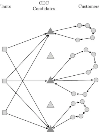
In the second stage, the consolidated products in the CDCs should be distributed to customers. Each customer is only visited by a single vehicle from a single CDC. In addition, all vehicles should return to their starting distribution centers after visiting a subset of customers (Fig 1). Therefore, this phase includes a capacitated multi-vehicle multi-depot routing problem should be solved. The two stages are considered in a single optimization framework. Two objectives are considered in this problem. The first objective is to minimize total costs including transportation costs from plants to CDCs, costs of opening CDCs and routing costs. The second objective function attempts to balance workloads on the vehicles. Each vehicle in the routing stage is associated with a maximum tour length which should not be exceeded. The second objective is, in fact, to balance the ratios of total distance traveled by each vehicle to the maximum tour length allowed for that vehicle. This idea derives from the fact that if the pure workload is considered, some vehicles, due to the difference in the maximum possible tour length, will be utilized in full capacity, while a low percentage of other vehicle’s capacity is occupied. On the other hand, taking into account the capacities results in a balanced routing plan in terms of vehicles’ tour lengths.
Fig 1 illustrates a sample solution to the problem under study. In this case, there are three plants, from which the products are delivered to the open CDCs. Three CDC locations are selected from five candidates in this solution. Finally, the commodities are delivered to the customers from intermediate points. Among the decisions should be made in the process of problem solving are assigning customers to CDCs, sequence of visiting the customers (route construction) and allocation of routes to available fleet.
Fig 1. A sample solution to the problem
3-Mathematical formulation
The mathematical formulation of the problem is presented in this section. The problem is formulated as a mixed-integer linear programming model.
253
3-1-Nomenclature
The nomenclature used to present the mathematical formulation of the model is as follows: 3-1-1-Sets
I {1, 2,, }:n Set of plants, indexed by i.
J {1, 2,, }:m Set of candidate CDC locations, indexed by
j
. K {m1,m 2, ,m q }: Set of customers, indexed byk
andk
. V {1, 2,, ,m m1,m 2, ,mq}: Set of candidate CDC locations, and customers, indexed by
v
and v V; J K T {1, 2,, }:p Set of commodity types, indexed by
t
. L{1, 2,, }:w Set of vehicles available in the second stage, indexed by
l
. 3-1-2-Parameters Sit: Maximum supply of product
k
by plant i. Dkt : Amount of product
t
demanded by customerk
.
C
tj:
Storage capacity of CDCj
for productt
.
TC
ijt:
Unit transportation cost of productt
from plant i to CDCj
. FCj: Opening cost candidate locationj
.
vv : Total distance/time between CDC/customerv
and CDC/customer v
.
B
t:
An upper-bound for the capacity of vehicles in the routing stage which can be assumed to be equal toMax CAP
{
t}
. tl:Cost of transporting one unit of commodity type
t
, for one unit of time/distance usingvehicle
l
. CAPlt:Capacity of vehicle
l
for product typet
.
l:
Maximum tour length allowed for vehiclel
. : An upper-bound for total tour length. It can be assumed to be equal to maximum of all allowed tour lengths of vehicles.
3-1-3-Decision variables
x
ijt:
Amount of productt
shipped from plant i to CDCj
.
1,
if a CDC is opened at candidate location ;
0,
othe
se
=
rwi .
j
j
y
1,
if customer is assigned to CDC ;
0,
otherwise.
k
j
r
1,
if customer is visited first in any route of CDC ;
0,
otherwise.
jk
k
j
1, if customer is the last node in any of CDC s routes;
0, other
wise
.
'
jk
k
j
1, if customer is visited just after customer in any of CDC 's routes;
0, otherwise.
jkk
k
k
j
254
rc
tvv:
Total cost of transportation of productt
from CDC/customerv
to CDC/customer v. ukt : Variable used to avoid sub-tours in the solutions and also to ensure the capacityconstraints of the vehicles in the routing stage.
1,
if customer is assigned to vehicle ;
0,
otherwise.
lk
k
l
lkk : Binary variable used to impose the following conditional statement on the model:2 1
lk lk lkk
.
min,
max:
Minimum and maximum lengths of the constructed tours.
e
k:
Positive variable used to prevent exceeding the maximum tour length allowed. It actually represents the distance traversed to reach customerk
.
er
k:
Positive variable which represents the ratio of tour length after visiting customerk
to maximum allowed tour length. òjkl: Positive variable, the value of which is equal to the distance/time that should be
traversed to reach to the depot from the last node in a tour. If customer
k
is not the last node in none of the tours of CDCj
, the value of òjkl is equal to 0.
k:
Auxiliary binary variable used to indicate whether nodek
is the last node in the shortest constructed tour (
k
1
) or not (
k
0
).
k:
Auxiliary binary variable used to indicate whether nodek
is the last node in the longest constructed tour.3-2- Mathematical model
The mathematical model of the problem is presented in this section. This model can be considered as an extension to the model presented by Martínez-Salazar et al. (2014). The proposed model is a multi-commodity two-echelon capacitated location routing problem considering a maximum tour length for each vehicle.
Two objective functions of minimizing costs and workload balance is considered in this model. The first objective function attempts to minimize total costs including fixed cost of CDCs, transportation costs from plants to CDCs and cost of delivering the commodities from CDCs to customers. The second objective function maximizes workload balance among vehicles in the second stage. To the best of our knowledge, in this paper, for the first time the capacity of the vehicles are considered in workload balance. The model tries to balance the utilization rates (ratio of tour length to maximum length allowed) of vehicles; instead of just to balance pure workloads.
1
:
t t t t t
ij ij j j jk kj kk
i j t j t j k t k k k k
Minz
TC
x
FC
y
rc
rc
rc
(1)
2 max min
Min z
(2)
Subject to:
t t
ij i
j
x S
i t,
(3)
t t
ij j j
i
x y C
j t,
(4)
t t
ij jk k
i k
x r D
j t,
(5)
1
jk j
r
255
jk jk
k k
j
(7)
:
jk jkk jk
k k k
r
j k
,
(8)
:
jk jkk jk
k k k
r
j k,
(9)
t t t
k k t jkk t k
j
u u B
B D
k k k
,
:
k t
,
(10)
t t t
k k lk l
l
D u
CAPk t,
(11)
2 2(1 )
lk lk lkk
l k k k
, ,
:
k
(12)
1
lk lk lkk
l k k k
, ,
:
k
(13)
1 (1 )
jk jk lkk
j j
l k k k
, ,
:
k
(14)
1
lk lk jkk
j
k k k
,
:
k l
,
(15)
1
lk lk jkk
j
k k k
,
:
k l
,
(16)
1
lk l
k
(17)
(1
)
t t
lk l
kk kk jkk
l j
rc
M
k k k
,
:
k t
,
(18)
1
t t
jk jk lk l jk
l
rc
M
j k t, ,
(19)
1
t t
kj kj lk l jk
l
rc
M
j k t, ,
(20)
lk lk lkk
l k k k
, ,
:
k
(21)
( ) ( )
k k kk jkk k k jk k
j j
e e
k k k
,
:
k
(22)
jk jk
k
jk
jk
j j
e
k
(23)
k lk l kj jk
l j
e
k
(24)
1
k
k lk
l
e
er
l k,
(25)
1
k
k lk
l
e
er
l k,
(26)
1
kj
jkl lk jk
l
ò
j k l, ,
(27)
1
kj
jkl lk jk
l
ò
j k l, ,
(28)
jkl
jkò
j k l, ,
(29)
min k jkl (1 jk)
j l j
er
ò
k
(30)
min k jkl (1 k)
j l
er
256
k jk
j
k
(32)
1
k k
(33)
max k jkl
j l
er
ò
k
(34)
max k jkl (1 k)
j l
er
ò
k
(35)
k jk
j
k
(36)
1
k k
k
(37)
min
,
max0
0
t ij
x
i j t, ,
{0,1}
j
y
j
, , {0,1}
jk jk jk
r
j k,
{0,1}
jkk
k k k
,
:
k
0
t k
u
k t,
{0,1}
lk
l k,
0
t kj
rc
j k t, ,
{0,1}
lkk
l k k k
, ,
:
k
,
0;
,
{0,1}
k k k k
e er
k
0
jkl
ò
j k l, ,
Objective function (1) attempts to minimize total costs. The second objective function (2) is applied to balance the ratios of tour length of vehicles to their maximum allowed tour length. Constraint (3) guarantees that the production capacities of plants are not exceeded for none of the product types. Constraint (4) ensures that no product is transported to a CDC, unless it is opened. It also imposes the capacity constraint of CDCs. Constraint (5) forces the solutions provided to satisfy all customers' demand. It also ensures that the input flow to and output flow from each CDC are equal. Constraint (6) implies each customer should be assigned to only one CDC. The equality constraint (7) implies that the number of routes started from a CDC must be equal to the number of routes ended at that CDC. The routes can only be constructed between the nodes assigned to the same CDC. Also, there are three conditions for a CDC, one of which should be chosen by the model: (i) the customer is visited immediately after a CDC, (ii) the customer is visited between two other customers, and (iii) the customer is the last node in a tour. Constraint (8) and (9) account for the mentioned issues. Constraints (10) and (11) provide the model with sub-tour elimination constraints as well as capacity constraints on the vehicles in the second (routing) stage. The restriction that all the nodes in a tour should be visited by only one vehicle is imposed on the model by constraints (12) and (13) and also constraints (18) to (22). Constraint (17) ensures that each customer should be assigned to exactly one vehicle. Costs of transportation from CDCs to customers and from customers to customers are calculated through constraints (15) to (17). The variable
e
k represents the distanced traveled in a tour to reach nodek
. Considering this issue constraints (23) and (25) are used in the model to calculate this variable. Constraints (26) to (30) are to establish the relationship among variableser
k,e
k andjkl
ò in order for the variables to take the designated values. The maximum and minimum tour lengths are calculated through constraints (31) to (35).
257
4-Solution approach
Since the problem under study is multi-objective in nature, it is not possible to find a single solution that optimizes both of the objective functions. Therefore, we utilize two solution methods, namely, Non-dominated Sorted Genetic Algorithm II (NSGA-II) (Deb et al., 2000) and Multi-objective PSO (MOPSO) (Coello Coello, 2002) in order to obtain the Pareto frontier, the set of non-dominated solutions. PSO and GA have shown successful performance in previous studies such as Hadian et al. (2019); Rabbani, Danesh et al. (2018). Hence, in this paper the multi-objective version of these algorithms are utilized to tackle the TLRP problem.
4-1-Solution representation
An efficient solution representation is needed to enhance the performance of meta-heuristic algorithms (Azadeh and Farrokhi-Asl, 2019). Accordingly, in this paper a new priority-based solution representation for the problem is proposed. Also, because the solution space of the problem studied is discrete in nature, an efficient mapping framework from the continuous solutions to continuous ones is required for the algorithms that are designed for continuous solution regions (e.g. MOPSO). The representation is mainly inspired by the approach proposed by Martínez-Salazar et al. (2014), but there are basic differences. Different operators of algorithms produce different solutions; the solution-n represesolution-ntatiosolution-n is desigsolution-ned isolution-n a way that the algorithms are provided with a chasolution-nce to explore whole solution region. For instance, a swap operator changes the priority of a plant, CDC candidate, customer or vehicle, resulting in a new solution to the problem.
The solution representation consists of the following parts: Priorities for plants
Priorities for CDC candidates Priorities for customers Priorities for vehicles
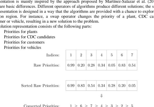
Fig 2. A sample conversion from raw real numbers to priorities
As mentioned before, for those algorithms designed for continuous solution regions, a mapping framework is needed. In these algorithms, the priorities produced are a set of real numbers (e.g. in the range of
0,1
), the highest value of which has the highest priority. Each solution consists of 4 sets of real numbers. To shed light on the conversion procedure from a raw set of real numbers to priorities, a sample conversion is illustrated in Fig 1. In the example, cell 1 is associated with the highest real number; therefore, it has the highest priority. The second highest priority is associated with cell 6. Hence cell 6 is the next priority. The procedure is repeated until the priority of all the entities in the set is determined.The procedure can be divided into three steps: Location of CDCs, transportation of commodities from plants to CDCs and finally delivering (routing) the commodities to the customers. It is noteworthy that all these parts are regarded as an integrated framework.
Initially, the CDC candidates with priorities lower than 0.5 are considered closed. Let m represent the number of open CDCs. In the next step, the customers are categorized into m clusters, based on
258
their
x
and ycoordinates. During the clustering process, the center of each cluster is determined as well.To assign the customers to CDCs, an assignment problem is solved. The assignment problem, one of the fundamental problems in operations research, consists of assigning some jobs to some candidates. Each job should be assigned to exactly one candidate, and each candidate can only have one job. Matching each pair of job-candidate is associated with a special cost. The total cost in this problem has to be minimized. Here, the CDCs represent the job candidates and the cluster centers represent the jobs. Each assignment is associated with a cost which is equal to the Euclidean distance between the center of clusters and CDCs. Once a distribution center is assigned to a cluster, all the customers of that cluster should be served by the CDC.
The CDC with the highest priority is chosen first. The customers assigned to the CDCs are served sequentially afterwards. Each customer has to be served by only one vehicle. Vehicle-customer assignments are conducted based on the priority of the vehicles. The customers are assigned to the highest-priority vehicle, until all the capacity of the vehicle is occupied (i.e. there is not enough space left for the next customer). Then, the vehicle is removed from the eligible list. There is an exception for the last vehicle; the capacity constraint is relaxed and the extra amount of demand served by the last vehicle is penalized.
The next step is to calculate total amount of commodities delivered via each CDC. The extra demand comparing to the capacity of the distribution centers is penalized afterwards. The next phase is the transportation phase. In this phase a multi-commodity transportation problem has to be solved. The transportation problem deals with some sources the provided commodities of which should be delivered to some destination. The demand of destinations and also the capacity of sources is defined in advance. In the last step total demand of each CDC is determined. The demand should be delivered from the plants. To solve the transportation problem a heuristic is proposed. The method is mainly inspired by the Hungerian algorithm (Kuhn, 1955). The priority-based heuristic approach is clarified in algorithm 1.
259 Algorithm 1: Transportation phase of the TLRP Data: Supply of the plants and demand of the CDCs.
Result: Amount of each commodity delivered from plants to CDCs. For each commodity type
t
doDefine
T
ijt as the amount of commodity typet
transported from plant i to CDCj
; LetT
ijt
0
for all i,j
andt
;Define
CDCLST
as the sorted list of open CDCs based on their priority; DefinePLANTLST
as the sorted list of plants based on their priority; Define RMit as the available commodity typet
at plant i;t t
i i
RM S for all i and
t
;Define
US
tj as the amount of unsatisfied demand of product typet
at CDCj
;t j
US
Amount of commodity typet
demanded by CDCj
; WhileCDCLST
is not empty doCURCDC
The first element inCDCLST
.;0
SATIS
;While
SATIS
1
doCURPLANT
The first element inPLANTLST
such thatt t
CURPLANT CURCDC
RM US ;
If
CURRENTPLNAT
is found then,
t t
CURPLANT CURCDC CURCDC
T
US
t t t
CURPLANT CURPLANT CURCDC
RM RM US ;
Remove
CURCDC
fromCDCLST
;1
SATIS
;If RMCURPLANTt 0 then
Remove
CURPLANT
fromPLANTLST
; Else,
t t
CURPLANT CURCDC CURPLANT
T
RM
;t t t
CURCDC CURCDC CURPLANT
US US RM ;
Remove
CURPLANT
fromPLANTLST
;Algorithm 2: The proposed NSGA-II Randomly generate the initial population;
Evaluate each solution in the population and assign a rank to each based on non-domination level; Let crowding distance of each solution be equal to the average distance of the two nearest solutions in the same rank to the current solution;
While termination criteria is not met do
Apply Crossover and Mutation operators on the current population and produce the temporary new population;
Calculate and update the non-domination levels and crowding distances;
Select from the new temporary population and the current population to generate the new population;
Store the solutions ranked #1 as the Pareto Frontier; Let current population = new population;
260
After penalizing the extra demand handled by CDCs and vehicles the fitness of the solution is determined in terms of both objective functions, namely, the balance and cost.
4-2-Proposed NSGA-II
Genetic Algorithm (GA) has been successfully utilized to solve LRPs Peng (2008) . Due to the advantages of GA over other solution algorithms, different variants of GA have been presented to tackle multi-objective problems. One of the most widely used multi-objective variants of GA is Non-dominated Sorting Genetic Algorithm II (NSGA-II), proposed by Deb et al. (2000). Among this method's advantages over its rivals are explicit diversity preservation mechanism, low overall complexity and elitism (which does not allow an already found Pareto optimal solution to be deleted) (Farrokhi-Asl et al., 2017; Rabbani et al., 2016)
The proposed NSGA-II is simply illustrated in algorithm 2. In the first step of the algorithm the initial population is randomly generated. The solutions in the population need to be evaluated and ranked based on their non-domination level. The solutions in the same rank neither dominate nor are dominated by one another. The crowding distance of each solution is determined afterwards. The crowding distance is indeed an indicator of how dense the solutions surrounding a particular solution are, which is equal to the average distance of its two neighboring solutions.
In all the iterations of the algorithm, the crossover and mutation operators are applied to the current population. Prior to crossover and mutation, it is essential first to select the parents. In this paper, a tournament selection method is applied to select the parents. Two solutions are chosen randomly; if they are not in the same rank the one with the higher rank is added to the pool; otherwise the one with better crowding distance is selected as a parent. This procedure continues until the size of the number of selected parents is equal to the size of the population. Using this method the chance of better solutions to be selected as a parent is higher. However, this chance for low-quality solutions is not equal to 0 (except for the lowest-quality solution).
Then, the consecutive parents are mated in order to produce new solutions. Different crossover operators have been proposed in previous research studies. The so-called order operator (OX1) is chosen as the crossover operator in this paper. In this method, first two crossover points are selected randomly. The offspring inherits the elements between the two points from the selected parent in the same position and order. The remaining elements are inherited from the other parent in the order in which they appear in the parent, beginning from the second crossover point (Starkweather, McDaniel, Mathias, Whitley, & Whitley, 1991).
Fig 3 demonstrates the OX1 crossover. Offspring1 inherits h e a b, , , , the string between the two crossover points, from Parent1, in the same order and place, and the remaining elements are inherited, in the same occurrence order, from Parent2. Using the same procedure the Offspring2 is generated. Mutation operators are used as a part of GAs in order to preserve the diversity of the populations. Different mutation operators are successfully used in different research studies. In addition, some researchers such as Farrokhi-Asl et al. (2017) used a mixture of different mutation methods. In order to ensure diverse solutions, in this paper a mixture of three mutation operators, namely, insertion, inversion and swap operators are used. They are chosen in iterations based on a uniform distribution. The insertion operator selects two genes at random and inserts the second gene right after the first
261
one. Inversion mutation procedure reverses the genes between two randomly selected points. Finally, the swap operator selects two genes randomly and swaps their position in the chromosome.
The crowding distance and non-domination level for each solution in the population is calculated is calculated afterwards. Based on elitism and crowding distance the population for the next iteration selected among the newly generated population and the current population (the population at the last iteration). Then, the rank #1 solution is stored as the Pareto frontier solutions. The main loop of the algorithm continues until a termination condition is met. The termination condition in this paper is reaching a predefined maximum number of iterations.
4-3-Proposed MOPSO
Particle Swarm Optimization is a nature-inspired population-based meta-heuristic proposed mainly designed and developed by R Eberhart and J Kennedy (1995); RC Eberhart and J Kennedy (1995); Eberhart, Simpson, and Dobbins (1996) . The algorithm is inspired by the behavior of bird flocks in search for food. In PSO, the flying of each particle is adjusted based on its own experience as well its companions' experience. This method has been developed in different ways. One of the most important variants of PSO is its multi-objective, MOPSO proposed by Coello Coello (2002). In their research study, Coello Coello (2002) show that MOPSO is capable of solving well-known difficult test problem in a reasonable amount of time.
The proposed MOPSO to solve the problem under study uses the solution representation illustrated in subsection 4.1. The steps of the algorithm are illustrated in algorithm 3.
Algorithm 3: The proposed MOPSO Generate initial population,
POP
; Let the speed of each particle,VEL
i
0
;Evaluate the particles and set
G
BEST equal to the set of non-dominated solutions inPOP
; LetP BEST
_
i
POP
i , for all particles;While termination condition is not met Do Calculate the velocity of each particle; Calculate the new position of each particle; Update P_BEST and G_BEST ;
First, the position of the particles needs to be initialized. For the purpose of simplicity, this step is done randomly in this paper. Then, the speed of particles is set to 0 as the initial value. The particles are evaluated afterwards and the set of global best solutions, G_BEST, is initialized with the non-dominated solutions so far. The personal best experiences are stored in P_BEST. The initial value for this parameter is the initial position of the particles,
POP
i . While the termination condition (maximum number of iterations in this paper) is not met, the algorithm, in all iterations, calculates the velocity of particles and accordingly the new positions. The velocity of particles is calculated through equation(38).
1 1
_
2 2(
)
i i i i i i
VEL
w VEL
C
r
P BEST
POP
C
r
LEAD
POP
(38)w
represents the inertia weight which is set to 0.5. This means one can control the relative effect of personal experience comparing to global experience.C
1 andC
2 are cognitive and social learning factors related to own success of a particle as well as neighborhood success, respectively.r
1 andr
2 represent two random numbers in the range of [0,1]. Based on (38), the new position of the particles is calculated using equation (39).i i i
POP
POP VEL
(39) Finally P_BEST and G_BEST are updated based on the generated particles.262
5-Computational results
In this section the computational results of the solution method proposed are discussed. In order to investigate the quality of the solution representation, it is applied in two different meta-heuristics, namely, multi-objective PSO (MOPSO) and also non-dominated sorted genetic algorithm (NSGA-II). To the best of our knowledge no set of test problems has been proposed for the problem studied. Therefore, in this paper test problems of different sizes are generated and solved. These test problems are generated randomly mainly based on the numerical experiments proposed by Martínez-Salazar et al. (2014).
5-1-Model validation
In order to validate the presented mathematical model in this paper, a small-sized problem is solved using GAMS software and the results are reported. The details of the test problem can be downloaded in the following link:
https://www.dropbox.com/sh/f7ntgh10gcrkkf4/AACicAyl_S3oaTXW7QvH67w5a?dl=0.
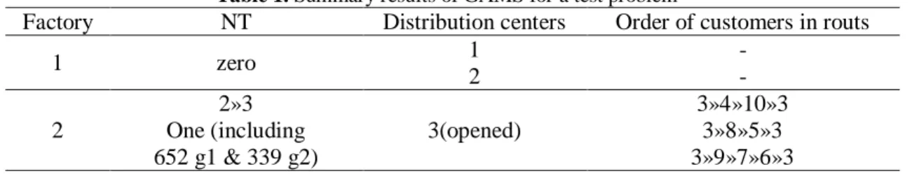
Numerical results obtained by solving the test problem show the validity of the proposed mathematical model. It should be mentioned that running time for solving this problem is about 1020 second. The results are summarized in tables 1 and 2.
Table 1. Summary results of GAMS for a test problem
Factory NT Distribution centers Order of customers in routs
1 zero 1 -
2 -
2
2»3 One (including 652 g1 & 339 g2)
3(opened)
3»4»10»3 3»8»5»3 3»9»7»6»3
Table 2. Objective values of GAMS for a test problem value
𝑓1 2.400001E+9
𝑓2 250
5-2-Solving test problems using metaheuristic algorithms
The test problems are classified into three groups of small-size, middle-size and large size instances. The plants, CDCs and customers are located randomly on a map of
200 50
. Other parameters such as capacities and demand of customers are determined randomly. The test problems finally resulted in 8 small size, 6 middle-size and 8 large-size problems. Table 33 illustrates the features and dimensions of the produced test problems.Table 3. Features and dimensions of the produced test problems
Small Middle Large
Number of Plants 2 4 6
Number of CDCs 3 5 8
Number of Clusters 8 10 15
Number of Vehicles 6 10 15
263
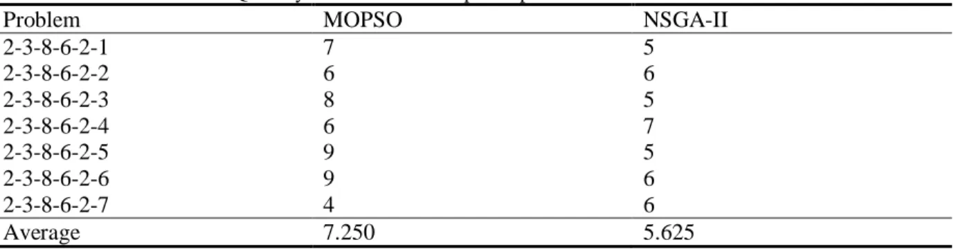
Table 4. Quantity of non-dominated points produced for the small instances
Problem MOPSO NSGA-II
2-3-8-6-2-1 7 5
2-3-8-6-2-2 6 6
2-3-8-6-2-3 8 5
2-3-8-6-2-4 6 7
2-3-8-6-2-5 9 5
2-3-8-6-2-6 9 6
2-3-8-6-2-7 4 6
Average 7.250 5.625
The test problems were named based on the structure of "nP-nCDC-nC-nV-nCom-Index", the first number arisen in the name is the number of plants. The second number shows the number of potential CDC sites and the third number is related to the number of customers. The fourth number represents the number of vehicles available and the next one is the number of commodity types. Finally, the last number is related to the index of the problem produced in each size.
All of the test problems were solved by applying the solution representation into MOPSO and NSGA-II. To evaluate and compare the performance of solution methods in multi-objective optimization different metrics have been introduced in previous researches Bazgan et al., (2015). In this paper the quantity of the solution vectors on the optimal Pareto frontier and also two other performance measure are used, namely, Size of the Space Covered (SSC) and K-Distance which are proposed by Zitzler and Thiele (1999) and Zitzler, Laumanns, and Thiele (2001), for the first time respectively.
The first performance measure used is the quantity of the non-dominated points on the Pareto frontier. This measure illustrates the ability of the method to produce efficient points. Table 4 - Table 6 demonstrate the quantity of points for the small, medium and large size instances respectively. It can be seen in Tables that based on this measure, in small instances the MOPSO provides better performance comparing to NSGA-II. By increase in the size of the problems, the algorithms show almost the same performance in medium instances, whereas in the large instances the NSGA-II significantly outperforms MOPSO.
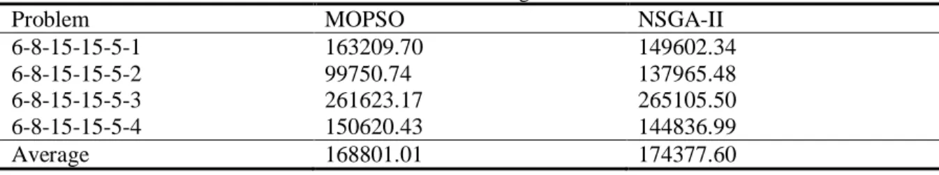
The second performance measure used is the size of space covered by the non-dominated points (SSC). The results of this measure for different instance sizes are illustrated in Table 7 to Table 9. It seems that NSGA-II has a better coverage in large instances rather than small and medium ones comparing to MOPSO.
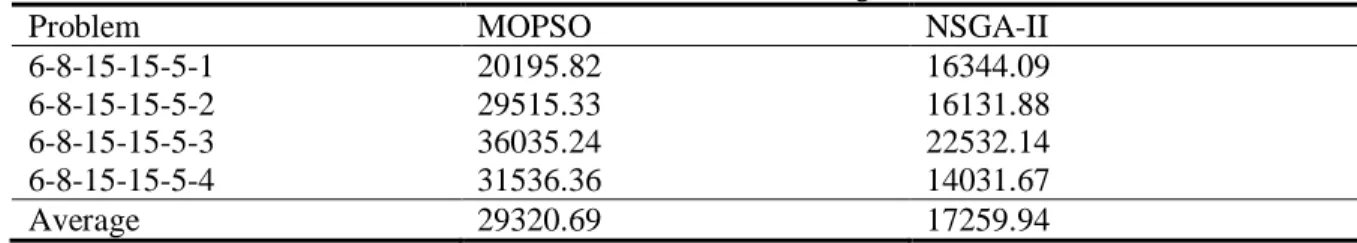
The last performance measurement studied is the k-distance measure. This value shows the density of the non-dominated points. In this paper average 3-distance is considered which means the distance to the third nearest dominant point. The results are depicted in Table 10 to 12.
Table 5. Quantity of non-dominated points produced for the medium instances.
Problem MOPSO NSGA-II
4-5-10-3-1 12 9
4-5-10-3-2 16 13
4-5-10-3-3 18 15
4-5-10-3-4 9 12
4-5-10-3-5 14 17
4-5-10-3-6 7 8
264
Table 6. Quantity of non-dominated points produced for the large instances
Problem MOPSO NSGA-II
6-8-15-15-5-1 17 23
6-8-15-15-5-2 15 24
6-8-15-15-5-3 17 28
6-8-15-15-5-4 11 15
Average 15 22.5
Table 7. SSC for small instances
Problem MOPSO NSGA-II
2-3-8-6-2-1 55499.53 50615.40
2-3-8-6-2-2 10982.23 9875.23
2-3-8-6-2-3 33231.50 29162.48
2-3-8-6-2-4 26543.87 27428.40
2-3-8-6-2-5 47349.55 52181.32
2-3-8-6-2-6 40705.45 37984.09
2-3-8-6-2-7 42263.40 39503.28
2-3-8-6-2-8 56732.10 62883.10
Average 39163.45 38704.16
Table 8. SSC for medium instances
Problem MOPSO NSGA-II
4-5-10-3-1 142797.30 123148.31
4-5-10-3-2 99206.37 107690.86
4-5-10-3-3 62731.06 89467.70
4-5-10-3-4 107748.59 98159.72
4-5-10-3-5 64928.77 41491.15
4-5-10-3-6 28125.93 18267.27
Average 84256.34 79704.17
The results of the 3-Distance measure suggest that the density of the non-dominated solutions produced by NSGA-II is more than those of MOPSO in small and medium instances, whereas in large instances MOPSO shows better performance in this measure.
Table 9. SSC for large instances
Problem MOPSO NSGA-II
6-8-15-15-5-1 163209.70 149602.34
6-8-15-15-5-2 99750.74 137965.48
6-8-15-15-5-3 261623.17 265105.50
6-8-15-15-5-4 150620.43 144836.99
Average 168801.01 174377.60
Table 10. 3-Distance measure for small instances
Problem MOPSO NSGA-II
2-3-8-6-2-1 12022.57 15431.20
2-3-8-6-2-2 16314.50 20535.50
2-3-8-6-2-3 14550.38 10647.40
2-3-8-6-2-4 24750.33 17360.14
2-3-8-6-2-5 14192.44 12933.40
2-3-8-6-2-6 12395.44 20917.00
2-3-8-6-2-7 11088.25 13962.33
2-3-8-6-2-8 12656.89 25796.20
265
Table 11. 3-Distance measure for medium instances
Problem MOPSO NSGA-II
4-5-10-3-1 27317.75 43704.00
4-5-10-3-2 15362.19 14591.38
4-5-10-3-3 17996.00 24501.13
4-5-10-3-4 21606.22 27695.33
4-5-10-3-5 14535.57 14785.53
4-5-10-3-6 23219.00 8889.38
Average 20006.12 22361.13
Table 12. 3-Distance measure for large instances
Problem MOPSO NSGA-II
6-8-15-15-5-1 20195.82 16344.09
6-8-15-15-5-2 29515.33 16131.88
6-8-15-15-5-3 36035.24 22532.14
6-8-15-15-5-4 31536.36 14031.67
Average 29320.69 17259.94
6-Conclusion
In this paper a variant of the two-echelon vehicle routing problem is studied. Multi-commodity demand and supply and heterogeneous fleet are some of the new assumptions considered in this study. Two objective functions of cost and work-load balance are taken into account. A new objective function is proposed to maximized work-load balance based on the capacity of the vehicles. The mathematical model of the problem is proposed in the form of a mixed integer linear programming model. To solve the problem a new and straightforward solution representation method is proposed. The solution method is applied via two different multi-objective evolutionary frameworks: NSGA-II and MOPSO. Eighteen new test problems were generated to investigate the efficacy of the solution method proposed. The results show that the solution method is able to generate acceptable solutions in reasonable amount of time. The comparison results between two methods applied illustrate that although MOPSO outperforms NSGA-II in small instances, however NSGA-II provides better estimation of the Pareto frontier in larger instances.
The model presented here can be useful for the companies which deliver their products to the demand nodes. In some cases, plants cannot deliver their products directly to demand nodes, motivating that, CDCs, operating as an intermediate point, are needed, to receive products from plants and to distribute products to customers. As such, this problem is a situation for city logistics companies in which heavy vehicles transporting final products from plants, are not allowed to reach clients located in the cities. On the other hand, vehicles arrive and unload their products in a CDC, usually located in cities periphery or some accessible places inside the city. By adding to number of established CDCs we can reach to more equitable distribution of commodities and this fact increases satisfaction level of logistics personnel. Conversely adding to number of CDCs increases cost of company and it is not desirable for senior managers of it. All in all, decision makers should perform a trade-off between these two factors and implement an appropriate optimum logistic network according to the importance of each goal.
References
Ai, T. J., & Kachitvichyanukul, V. (2009). Particle swarm optimization and two solution representations for solving the capacitated vehicle routing problem. Computers & Industrial Engineering, 56(1), 380-387.
Aikens, C. H. (1985). Facility location models for distribution planning. European journal of operational research, 22(3), 263-279.
266
Ambrosino, D., & Scutella, M. G. (2005). Distribution network design: New problems and related models. European journal of operational research, 165(3), 610-624.
Azadeh, A., & Farrokhi-Asl, H. (2019). The close–open mixed multi depot vehicle routing problem considering internal and external fleet of vehicles. Transportation Letters, 11(2), 78-92.
Bazgan, C., Jamain, F., & Vanderpooten, D. (2015). Approximate Pareto sets of minimal size for multi-objective optimization problems. Operations Research Letters, 43(1), 1-6.
Boccia, M., Crainic, T. G., Sforza, A., & Sterle, C. (2010). A Metaheuristic for a Two Echelon Location-Routing Problem. Paper presented at the SEA.
Chen, C.-T. (2001). A fuzzy approach to select the location of the distribution center. Fuzzy sets and systems, 118(1), 65-73.
Coello Coello, C. A. (2002). MOPSO: A proposal for multiple objective particle swarm optimization. Paper presented at the Proceedings of the 2002 Congress on Evolutionary Computation (CEC 2002). Crainic, T. G., Mancini, S., Perboli, G., & Tadei, R. (2008). Clustering-based heuristics for the two-echelon vehicle routing problem. Montreal, Canada, Interuniversity Research Centre on Enterprise Networks, Logistics and Transportation, 17, 26.
Crainic, T. G., Sforza, A., & Sterle, C. (2011). Tabu search heuristic for a two-echelon location-routing problem: CIRRELT.
Crainic, T. G., Storchi, G., & Ricciardi, N. (2007). Models for evaluating and planning city logistics transportation systems: CIRRELT.
Dukkanci, O., Kara, B. Y., & Bektaş, T. (2019). The green location-routing problem. Computers & Operations Research, 105, 187-202.
Dalfard, V. M., Kaveh, M., & Nosratian, N. E. (2013). Two meta-heuristic algorithms for two-echelon location-routing problem with vehicle fleet capacity and maximum route length constraints. Neural Computing and Applications, 23(7-8), 2341-2349.
Deb, K., Agrawal, S., Pratap, A., & Meyarivan, T. (2000). A fast elitist non-dominated sorting genetic algorithm for multi-objective optimization: NSGA-II. Paper presented at the International Conference on Parallel Problem Solving From Nature.
Demircan-Yildiz, E. A., Karaoglan, I., & Altiparmak, F. (2016). Two Echelon Location Routing Problem with Simultaneous Pickup and Delivery: Mixed Integer Programming Formulations and Comparative Analysis. Paper presented at the International Conference on Computational Logistics. Drexl, M., & Schneider, M. (2015). A survey of variants and extensions of the location-routing problem. European journal of operational research, 241(2), 283-308.
Eberhart, R., & Kennedy, J. (1995). A new optimizer using particle swarm theory In: Proceedings of the sixth international symposium on micro machine and human science, vol 43 IEEE. New York. Eberhart, R., & Kennedy, J. (1995). Particle swarm optimization, proceeding of IEEE International Conference on Neural Network. Perth, Australia, 1942-1948.
Eberhart, R., Simpson, P., & Dobbins, R. (1996). Computational Intelligence PC Tools. In: Academic Press Professional, Inc.
Farham, M. S., Süral, H., & Iyigun, C. (2018). A column generation approach for the location-routing problem with time windows. Computers & Operations Research, 90, 249-263.
Farrokhi-Asl, H., Tavakkoli-Moghaddam, R., Asgarian, B., & Sangari, E. (2017). Metaheuristics for a bi-objective location-routing-problem in waste collection management. Journal of Industrial and Production Engineering, 34(4), 239-252.
267
Gonzalez-Feliu, J., Perboli, G., Tadei, R., & Vigo, D. (2008). The two-echelon capacitated vehicle routing problem.
Hadian, H., Golmohammadi, A., Hemmati, A., & Mashkani, O. (2019). A multi-depot location routing problem to reduce the differences between the vehicles’ traveled distances; a comparative study of heuristics. Uncertain Supply Chain Management, 7(1), 17-32.
Hassanzadeh, A., Mohseninezhad, L., Tirdad, A., Dadgostari, F., & Zolfagharinia, H. (2009). Location-routing problem. In Facility Location (pp. 395-417): Springer.
Jacobsen, S. K., & Madsen, O. B. (1980). A comparative study of heuristics for a two-level routing-location problem. European journal of operational research, 5(6), 378-387.
Kuhn, H. W. (1955). The Hungarian method for the assignment problem. Naval Research Logistics (NRL), 2(1‐2), 83-97.
Lan, Y.-h., & Li, Y.-s. (2010). The method of cluster and entropy apply in city distribution center location. Paper presented at the Educational and Network Technology (ICENT), 2010 International Conference on.
Laporte, G., & Nobert, Y. (1981). An exact algorithm for minimizing routing and operating costs in depot location. European journal of operational research, 6(2), 224-226.
Martínez-Salazar, I. A., Molina, J., Ángel-Bello, F., Gómez, T., & Caballero, R. (2014). Solving a bi-objective transportation location routing problem by metaheuristic algorithms. European journal of operational research, 234(1), 25-36.
Nagy, G., & Salhi, S. (2007). Location-routing: Issues, models and methods. European journal of operational research, 177(2), 649-672.
Nguyen, V.-P., Prins, C., & Prodhon, C. (2010). A Multi-Start Evolutionary Local Search for the Two-Echelon Location Routing Problem. Hybrid Metaheuristics, 6373, 88-102.
Nikbakhsh, E., & Zegordi, S. (2010). A heuristic algorithm and a lower bound for the two-echelon location-routing problem with soft time window constraints. Scientia Iranica. Transaction E, Industrial Engineering, 17(1), 36.
Or, I., & Pierskalla, W. P. (1979). A transportation location-allocation model for regional blood banking. AIIE transactions, 11(2), 86-95.
Peng, Y. (2008). Integrated Location-Routing Problem Modeling and GA Algorithm Solving. Paper presented at the Intelligent Computation Technology and Automation (ICICTA), 2008 International Conference on.
Perboli, G., & Tadei, R. (2010). New families of valid inequalities for the two-echelon vehicle routing problem. Electronic notes in discrete mathematics, 36, 639-646.
Punyim, P., Karoonsoontawong, A., Unnikrishnan, A., & Xie, C. (2018). Tabu search heuristic for joint location-inventory problem with stochastic inventory capacity and practicality constraints. Networks and Spatial Economics, 18(1), 51-84.
Rabbani, M., Danesh Shahraki, S., Farrokhi-Asl, H., & Lim, F. W. (2018). A new multi-objective mathematical model for hazardous waste management considering social and environmental issues. Iranian Journal of Management Studies, 11(4), 823-859.
Rabbani, M., Farrokhi-Asl, H., & Ameli, M. (2016). Solving a fuzzy multi-objective products and time planning using hybrid meta-heuristic algorithm: Gas refinery case study. Uncertain Supply Chain Management, 4(2), 93-106.