The Forward Modeling of the Inner Kinetochore in S. cerevisiae
By AyushDoshi
Senior Honors Thesis Department of Biology
University of North Carolina at Chapel Hill
April 251\ 2019
Abstract
The kinetochore is a large protein complex that connects chromosomes to the mitotic
spindle to ensure proper cell division. The kinetochore can be divided into two significant
regions: the inner kinetochore, which includes proteins that interact with DNA; and the outer
kinetochore, which includes microtubule-binding proteins. Due to the crucial nature of the
kinetochore, it finds itself at the center of many studies aimed at characterizing the complex.
However, similar to other forms of biological research, analysis and comparison of microscopy
images present a significant investment of manpower and time. We propose a novel pipeline
for image analysis tailored to the kinetochore that provides efficient feature extraction and
insight into its 3D structure through the use of kernel classifiers and convolutional neural
networks (CNN). The differentiation between inner and outer kinetochore structures along
with the initial convolution of the inner kinetochores’ 3D structure was used as a test case to
display the usefulness of the pipeline. Its success attests to the usefulness of this pipeline as
not only an effective method to analyze and understand the differences that occur structurally
at the protein level, but also as an extremely time efficient one.
Introduction
Two of the most vital events that a cell can undergo are mitosis and meiosis. Due to
the importance of these events to the cell, many proteins are irreplaceable in the two
pro-cesses, of which a subset of proteins make up the protein complex known as the kinetochore
[1]. Composed of more than 100 proteins, this cylindrical-shaped conglomerate of proteins
assembles at the centromeres of chromatids in eukaryotic cells and binds to the (+) - end of
the microtubules [2, 3]. The kinetochore complex also plays an important role in the spindle
assembly checkpoint by confirming that all the chromosomes are attached to the spindle in
a bipolar orientation prior to the separation of the sister chromatids [4].
the outer kinetochore [5]. The inner kinetochore is composed of proteins that are localized
close to the chromatin, interacting with the DNA. The proteins that are part of the inner
kinetochore inS. cerevisiae include Cse4, Ame1, and Okp1 [6, 7]. The outer kinetochore, on
the other hand, is composed of proteins that are localized close to microtubules and contains
the microtubule-binding domain of the kinetochore complex. The proteins that are part of
the outer kinetochore in S. cerevisiae include Nuf2, Ndc80, and Spc24 [8].
S. cerevisiae poses a very useful model for the kinetochore complex for several
rea-sons. Primarily, many of the proteins in the kinetochore complex ofS. cerevisiae have direct
homologs to other eukaryotic organisms, most importantly humans, allowing for
understand-ings in S. cerevisiae to be translated to humans with relative ease [9]. Furthermore, a large
body of work on the genetics and nuclear dynamics of S. cerevisiae already exists, which
provides a useful foundation that can be further expounded upon. Lastly, while the general
structure of the kinetochore complex of S. cerevisiae is similar to that of other eukaryotic
organisms, simplifications in the structure allow for easier modeling and analysis, such as
the one-to-one binding nature of a kinetochore to a microtubule that is not present in higher
eukaryotic organisms [10].
Much work on understanding the kinetochore in the S. cerevisiae model has been
previously done, which include analyzing the 3D structure through electron microscopy,
characterizing key kinetochore protein interactions, and identifying systematic differences
between inner and outer kinetochore proteins [6, 7, 10, 11]. Nonetheless, further research is
still being done to address the many questions that remain about the kinetochore complex.
Yet, the process of acquisition, segmentation, and analysis of microscopy images to gain
insight about the kinetochore is often limited to an inefficient and slow binary comparison
of features filled with human bias, and does not provide any avenue for future classification
of phenotypes or structures without spending large amounts of time and resources to train
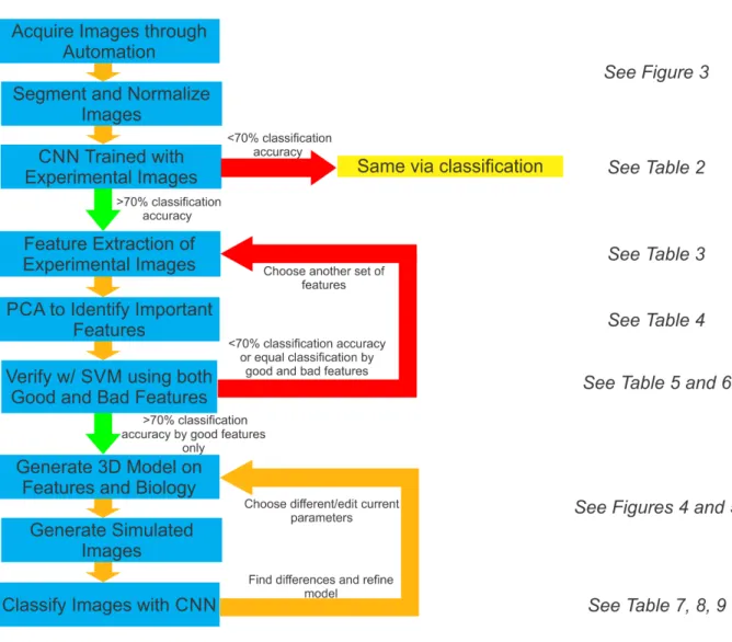
an individual to do so by eye. To address these concerns and provide a method that is more
based on publicly available segmentation algorithms, deep learning and machine learning
techniques, and basic statistical procedures [12].
The pipeline begins by taking images and segmenting out the foci of two conditions
through an automated sub-process and pre-processing them. An initial test on whether the
physical differences of the two conditions differ is then run by using a CNN. If the neural
network fails to successfully both train and categorize the two conditions correctly at an
accuracy of 70% or higher, then the two conditions are deemed to have the same physical
characteristics. However, if the neural network does successfully both train and categorize
the two conditions, then the features that are thought to be important are extracted from
the two sets of images. Principal component analysis is then used to identify the features
that are of greatest importance to the distribution, which are then validated through
suc-cessful segregation of the two distributions using a support vector machine. If the support
vector machine fails to correctly categorize the two conditions at an accuracy greater than
70% based on the features shown to be important, or if support vector machines trained
on important and unimportant features have equal accuracy, then additional features are
chosen and the process of extraction, identification, and validation of important features is
repeated. However, if the validation is successful and only the important features build a
valid segregating hyperplane, those features are then used as the basis for the development
of a 3D model that can output simulated microscope images. The accuracy of the 3D model
is then explored through successful classification of the simulated images by a CNN that is
trained on experimental images or the classification of experimental images by a CNN that is
trained on simulated images. This procedure of building a model and analyzing it is repeated
to develop more accurate and useful models that can then be used to better understand the
important characteristics of the point of interest.
To test the pipeline and its effectiveness in discerning differences in physical
character-istics as well as its ability to generate 3D models, we used a test case comparing the inner
conditions provide a useful test case as there is a large body of work that has been done in
characterizing the different features of these two regions [6, 7, 11]. Furthermore, by building
a 3D model of the inner kinetochore, we test the accuracy of the current model of the inner
kinetochore and propose grounds for alternatives.
Methods
Segmentation and Normalization of Experimental Images
Population, seven Z-plane image stacks of Spc29-RFP, N-Nuf2-GFP and Spc29-RFP,
Cse4-GFP yeast strains were acquired with a Nikon Eclipse Ti TE2000-U inverted fluorescent
microscope using a Nikon Apo 1.4 NA 100x objective, MetaMorph 7.8 software, Hamamatsu
Orca Flash 4.0 LT camera, and LumenCor Aura Light Engine. The cells in the images were
segmented using a MATLAB program, CellStarSelect.m, based on the CellStar algorithm for
identifying budding yeast in brightfield microscopy, creating a 50 x 50-pixel image around
each cell. The seven-step 50 x 50-pixel stack of each cell was then condensed into a
sin-gle plane using a maximum projection approach and had their intensity values normalized
between 0 and 4095 intensity units. Duplicates of the images were generated by either
ro-tating the images 90, 180, or 270 degrees, flipping the image across the y-axis, or both, thus
generating an additional 7 different orientations of the initial image and increasing the size
of the data-set. The images then underwent a background subtraction procedure and were
de-noised using a low-pass 2D Wiener filter.
Training and Testing of a Convolutional Neural Network
Image sets of the categories of interest were randomized and split into training,
val-idation, and testing data-stores, with 56% of the images used for training, 24% used for
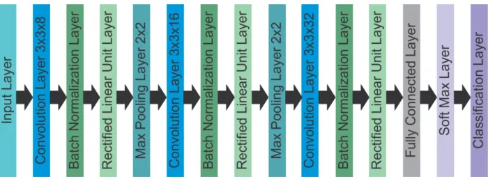
validation, and 20% used for testing. The architecture of the CNN contained 13 layers with
times, with the first layer consisting of a 3 x 3 convolutional layer with a stride of 1 and 8,
16, and 32 filters respectively. The second layer was a batch normalization layer, the third
layer was a rectified linear unit layer, and the fourth layer was a 2 x 2 max-pooling layer
with a stride of 2. However, on the final repetition of the 4 layers, the fourth layer was a
fully connected layer that fed into a SoftMax layer. The training used stochastic gradient
descent with momentum as well as the associated default values for this method in
MAT-LAB, with the exception of the initial learning rate set to 0.01, the max epochs set to 20,
and a validation frequency set to 30 iterations. The CNN was then tested with the images
in the testing data-store and a confusion chart was generated.
Feature Extraction and Principal Component Analysis
Features of interest (Table 1) of the 50 x 50-pixel maximum projections of the cells
were calculated and extracted using a MATLAB program, PCAFeatureExtraction.m. The
output produced was eigenvectors, which defined the axes of the principal components, and
the associated eigenvalues, which represented the percent of total variance explained by
the eigenvector. Features were considered important if they compose more than 80% of any
principal component that itself explains the initial 99.9% of the total variance of the data-set.
Remaining features were considered unimportant.
Training and Testing Binary Gaussian Kernel Classification Models
Observations and associated data from the feature extraction were randomized and
split into training and testing data-stores, with 70% of the images used for training and the
remaining 30% used for testing. The training set was then used to train a binary Gaussian
kernel-based classification model using a MATLAB program, TrainAndTest01Classifier.m.
The classifier used a support vector machine-based response range and a deviance loss
func-tion with a variable regularizafunc-tion term strength, kernel scale parameter, and the number of
accuracy was calculated.
3D Modeling of the Kinetochore and Simulated Image Generation
A MATLAB program, KineticButShakeless.mlapp, was used to generate 3D structures
of the kinetochore by simulating fluorophore organization. The fluorophores were simulated
as spheres whose 3D coordinates were determined by a cylindrical kinetochore model and
parameter values that were user-defined based on the desired structure at the time. The
program outputted a .xml file that contained the fluorophore locations that was then read
and converted into simulated microscope images by Microscope Simulator 2 [13].
Results
Inner and Outer Kinetochore Complexes Differ in their Microscope Images
To initially determine whether the images inner and outer kinetochore complexes differ
inherently, images of Spc29-RFP, GFP-Nuf2 (outer kinetochore) and Spc29-RFP, Cse4-GFP
(inner kinetochore) were acquired through the automated image acquisition pipeline. The
automated process of acquiring, segmenting, and preprocessing images of Spc29-RFP,
N-Nuf2-GFP and Spc29-RFP, Cse4-GFP generated 4,224 and 2,880 images respectively (Figure
3). Of the 4,224 images of Nuf2, 2,880 were randomly selected to allow for a balanced
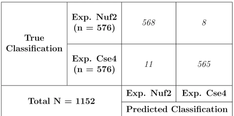
data-set, which was piped into the CNN. The neural network was able to distinguish and categorize
inner kinetochore images from outer kinetochore images at a 98.4% testing accuracy (Table
2), suggesting that the Nuf2 and Cse4 differ in the physical characteristics of their microscope
Spot Height, Standard Deviation in X, and Distance to Spindle Pole Body are
Important Features for Distinguishing Inner and Outer Kinetochore Complexes
To identify features that are important in distinguishing inner and outer kinetochore
images, features of interest were extracted from the population of Nuf2 and Cse4 images
(Table 3) and principal component analysis was done on the raw data (Table 4). Based on
the analysis results, the key features that are important for the identification of the inner
and outer kinetochores are spot height, the standard deviation of the pixel distribution of
the kinetochore foci along the x-axis, and the distance between the brightest pixel of the
kinetochore foci to the brightest pixel of its closest spindle pole body foci. These results agree
with what is already known about the inner and outer kinetochore complexes, supporting the
reliability of this method in finding patterns in the differences between the two regions [11].
Furthermore, supplementary analysis on images of the inner and outer kinetochore that were
not normalized to a 12-bit image as part of the preprocessing found that the mean intensity
of the pixels near the brightest pixel of a foci between the inner and outer kinetochore images
prove to be useful in identifying the two conditions, a result that has also been previously
known but acquired in a significantly shorter timeframe [14].
The importance of these features was tested by training two classification models:
one model on the features found to be important and the other on the remaining features.
The validation of important features’ usefulness proved successful as the classifier trained on
important features had an accuracy of 97.2% (Table 5) in its testing phase while the classifier
trained on unimportant features had an accuracy of 54.8% (Table 6) in its testing phase,
supporting the importance of the useful features in explaining the differences between the
Current Model of the Inner Kinetochore Fails to Match Experimental Inner
Kinetochore Images
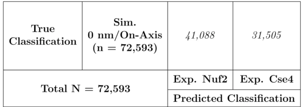
To gain further insight into the underlying 3D structure of the inner kinetochore,
sim-ulated images were developed and analyzed that were based on the current model of the
kinetochore where the inner kinetochore complexes taper to a point that is in line with the
central axis of the microtubule, often referred to as the taper/on-axis model (Figure 4). For
these images, the diameter of the spindle was set to 250 nm, with each microtubule having
a diameter of 25 nm, and the microtubule ends were staggered in a uniform distribution
± 100 nm from the central line. However, when the simulated images of the inner
kineto-chore were classified by the initial experimentally trained CNN, the simulated images were
poorly classified with an accuracy of 43.4% (Table 7), suggesting that the taper model is not
representative of the inner kinetochore structure.
Radially Displaced Model of the Inner Kinetochore Better Matches
Experimen-tal Inner Kinetochore Images
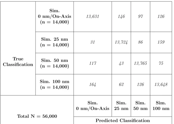
To further explore the 3D structure of the inner kinetochore, simulated images were
generated that had varying radial displacements of 25, 50, and 100 nm. These values
rep-resent the radial distance perpendicular to the spindle axis that the binding center of the
inner kinetochore is shifted relative to its microtubule’s central axis (Figure 5). These image
sets, along with the original on-axis, 0 nm radial displacement organization, were then used
to train a CNN, which resulted in a 97.8% accuracy during the testing phase (Table 8). The
experimentally-acquired images of the inner kinetochore were then categorized by the CNN
trained on the simulated images of different radial displacements in the effort to understand
which category the experimental images best fit into. The CNN categorized the majority of
experimental images in the 100 and 50 nm radial displacement bins and a small number in
the 0 nm and 25 nm bins (Table 9), suggesting that a radial displaced organization better
Discussion
Successful Identification of Differences and Key Features Between Inner and
Outer Kinetochore
The pipeline was able to identify the existence of a physical characteristic difference
between the microscope images of inner and outer kinetochore at an accuracy of 98.4%.
Furthermore, the pipeline was able to identify and validate useful features based on the
principal component analysis of raw feature data, identifying spot height, standard deviation
along the X-axis, and the distance of a kinetochore foci to its closest spindle pole body as key
physical aspect to distinguish inner and outer kinetochores, features that have been shown
in previous work to be valuable in differentiating the two conditions from one another.
The ability for the pipeline to confirm the findings of previous kinetochore research in S.
cerevisiae supports the accuracy of the pipeline, while the ability for the pipeline to come to
these conclusions over the span of only one month including data acquisition, supports the
time and resource efficiency of the pipeline, allowing for the conclusion of a successful test
case.
Radially Displaced Model Better Fits Experimental Images of the Inner
Kine-tochore than On-Axis/Taper Model
The pipeline was also used to delve into the 3D structure of the kinetochore and gain
insight into its organization. Based on the classifications of simulated on-axis model images
by the CNN trained on experimental images of Cse4 and Nuf2, the tapering organization
of the inner kinetochore is not well supported as the underlying organization of the inner
kinetochore proteins. This lack of support is further seen by the classification of experimental
inner kinetochore images by the CNN trained on 0, 25, 50, and 100 nm radial displacement
images, where the significant majority is classified in the 50 and 100 nm bins. This allows
of the inner kinetochore. The future direction of work is now aimed at refining the model
through the consideration of having some of the arms of the inner kinetochore complex be
unbound and able to freely rotate as indicated by recent research, and reanalyzing the model
[15].
Acknowledgements
I would like to thank the following: Dr. Kerry Bloom, who has been a wonderful
Personal Investigator by seeing something valuable in a side project and supporting it; Dr.
Josh Lawrimore, who was an amazing mentor who provided not only useful guidance and
a wall for me to bounce ideas off, but honest critiques that helped me make my work as
fully fleshed out as possible; Bloom Lab and funding from the NIH to KB (R37GM32238)
for providing the necessary resources and funds to explore and build upon the idea; and
lastly Dr. Russell M. Taylor II, who provided valuable critiques of deep learning and useful
insight on the potential pitfalls of the original pipeline, allowing for me to make it as robust
as possible.
References
1. Cleveland, D. W., Mao, Y. & Sullivan, K. F. Centromeres and Kinetochores: From
Epigenetics to Mitotic Checkpoint Signaling. Cell 112, 407–421.issn: 0092-8674 (Feb.
2003).
2. Bloom, K., Sharma, S. & Dokholyan, N. V. The path of DNA in the kinetochore.
Current biology : CB 16, R276–8.issn: 0960-9822 (Apr. 2006).
3. Cheeseman, I. M. & Desai, A. Molecular architecture of the kinetochore–microtubule
4. Lara-Gonzalez, P., Westhorpe, F. G. & Taylor, S. S. The Spindle Assembly Checkpoint.
Current Biology 22, R966–R980. issn: 0960-9822 (Nov. 2012).
5. Cheeseman, I. M., Drubin, D. G. & Barnes, G. Simple centromere, complex kinetochore:
linking spindle microtubules and centromeric DNA in budding yeast. The Journal of
cell biology 157, 199–203. issn: 0021-9525 (Apr. 2002).
6. Stoler, S., Keith, K. C., Curnick, K. E. & Fitzgerald-Hayes, M. A mutation in CSE4, an
essential gene encoding a novel chromatin-associated protein in yeast, causes
chromo-some nondisjunction and cell cycle arrest at mitosis. Genes & development 9,573–86.
issn: 0890-9369 (Mar. 1995).
7. Pot, I.et al.Spindle Checkpoint Maintenance Requires Ame1 and Okp1. Cell Cycle 4,
1448–1456. issn: 1538-4101 (Oct. 2005).
8. He, X., Rines, D. R., Espelin, C. W. & Sorger, P. K. Molecular analysis of
kinetochore-microtubule attachment in budding yeast. Cell 106, 195–206. issn: 0092-8674 (July
2001).
9. Kitagawa, K. & Hieter, P. Evolutionary conservation between budding yeast and human
kinetochores.Nature Reviews Molecular Cell Biology 2,678–687.issn: 1471-0072 (Sept. 2001).
10. Peterson, J. B. & Ris, H. Electron-microscopic study of the spindle and chromosome
movement in the yeast Saccharomyces cerevisiae. Journal of cell science 22, 219–42.
issn: 0021-9533 (Nov. 1976).
11. Haase, J., Stephens, A., Verdaasdonk, J., Yeh, E. & Bloom, K. Bub1 Kinase and Sgo1
Modulate Pericentric Chromatin in Response to Altered Microtubule Dynamics.
Cur-rent Biology 22,471–481. issn: 09609822 (Mar. 2012).
12. Versari, C. et al. Long-term tracking of budding yeast cells in brightfield microscopy:
CellStar and the Evaluation Platform. Journal of The Royal Society Interface 14,
13. Quammen, C. W. et al. FluoroSim: A Visual Problem-Solving Environment for
Flu-orescence Microscopy. Eurographics Workshop on Visual Computing for Biomedicine
2008, 151–158. issn: 2070-5778 (Jan. 2008).
14. Lawrimore, J., Bloom, K. S. & Salmon, E. Point centromeres contain more than a single
centromere-specific Cse4 (CENP-A) nucleosome.The Journal of Cell Biology 195,573– 582. issn: 0021-9525 (Nov. 2011).
15. Yoo, T. Y. et al. Measuring NDC80 binding reveals the molecular basis of
tension-dependent kinetochore-microtubule attachments. eLife 7. issn: 2050-084X. doi:10 .
7554/eLife.36392.https://elifesciences.org/articles/36392 (July 2018).
16. Joglekar, A. P., Bloom, K. & Salmon, E. In Vivo Protein Architecture of the Eukaryotic
Kinetochore with Nanometer Scale Accuracy.Current Biology 19,694–699. issn:
0960-9822 (Apr. 2009).
17. Gibeaux, R., Politi, A. Z., N´ed´elec, F., Antony, C. & Knop, M. Spindle pole
body-anchored Kar3 drives the nucleus along microtubules from another nucleus in
prepa-ration for nuclear fusion during yeast karyogamy. Genes & development 27, 335–49.
Figures
Figure 2. Graphical representation of the architecture used for the CNN.
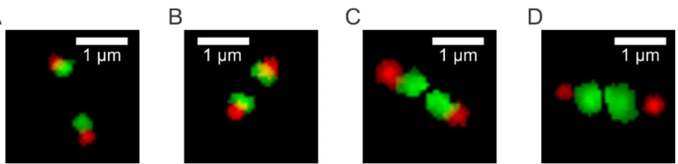
Figure 5. Model organization and representative GFP fluorescent images of the inner kine-tochore at 25, 50, and 100 nm radial displacement. (a) - (c) Side view of the 3D model for 25, 50, and 100 nm respectively, with Cse4 as green circles, N-terminal of Nuf2 as blue circles forming a ring around the microtubule, Spc29 as red circles, and the measurement that represents radial displacement. N-terminal of Nuf2 is only shown to allow for easier visualization of the radial displacement of the inner kinetochore chromatin binding point and is not generated in the simulated microscope images. (e) - (g) Volumetric model of the 25, 50, and 100 nm radial displacement organizations respectively that will be used for image generation, depicting the two pairs of Cse4 and Spc29, which can be seen in (h)-(j) the respective simulated microscope images.
Tables
Feature Description
Spot height
Full-width-half-max of the maximum projection of the 7 x 15 region about the brightest pixel of the kinetochore foci
perpendicular to the spindle.
Distance to spindle pole body
Euclidean distance between the brightest pixel of the kinetochore and the brightest pixel of its closest spindle pole
body, normalized by the length of the spindle axis.
Standard deviation in X direction
Standard deviation of the distribution generated from a line-scan of a kinetochore foci parallel to the spindle.
Standard deviation in Y direction
Standard deviation of the distribution generated from a line-scan of a kinetochore foci perpendicular to the spindle.
K-K Distance Euclidean distance between the brightest pixels of the two kinetochore foci, normalized by the length of the spindle axis.
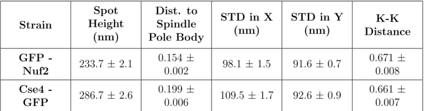
Table 1. Features of interest and description of their calculation.
True Classification
Exp. Nuf2
(n = 576) 568 8
Exp. Cse4
(n = 576) 11 565
Total N = 1152 Exp. Nuf2 Exp. Cse4 Predicted Classification
Strain Spot Height (nm) Dist. to Spindle Pole Body
STD in X (nm)
STD in Y (nm)
K-K Distance
GFP
-Nuf2 233.7 ± 2.1
0.154 ±
0.002 98.1 ± 1.5 91.6 ± 0.7
0.671 ±
0.008
Cse4
-GFP 286.7 ± 2.6
0.199 ±
0.006 109.5 ±1.7 92.6 ± 0.9
0.661 ±
0.007
Table 3. Mean and standard error of the 5 features for Cse4 and Nuf2 experimental images.
Principal Axis Spot Height Dist. to Spindle Pole STD in X STD in Y K-K Distance % Explained
1 0.998 0.002 -0.001 3×10⁻⁶ 1×10⁻⁵ 86.7%
2 6×10⁻⁴ 0.824 0.637 -0.003 2×10⁻⁴ 9.62% 3 −2×10⁻⁸ 0.438 0.871 9×10⁻⁸ −1×10⁻⁷ 3.61% 4 5×10⁻⁴ 6×10⁻⁵ 0.027 0.513 -0.634 0.04%
5 1×10⁻⁸ -0.007 −3×10⁻⁴ 0.0975 0.803 0.03%
Table 4. Composition of each feature and the percent of the total variance explained for each principal axis calculated by the principal component analysis.
True Classification
Exp. Nuf2
(n = 380) 367 13
Exp. Cse4
(n = 380) 9 371
Total N = 760 Exp. Nuf2 Exp. Cse4 Predicted Classification
True Classification
Exp. Nuf2
(n = 380) 342 38
Exp. Cse4
(n = 380) 306 74
Total N = 760
Exp. Nuf2 Exp. Cse4 Predicted Classification
Table 6. Confusion matrix of the testing data-set for the kernel classifier based on STD in Y and K-K Distance features, depicting the successful and erroneous classifications.
True Classification
Sim. 0 nm/On-Axis
(n = 72,593)
41,088 31,505
Total N = 72,593 Exp. Nuf2 Exp. Cse4 Predicted Classification
True Classification
Sim. 0 nm/On-Axis
(n = 14,000)
13,631 146 97 126
Sim. 25 nm
(n = 14,000) 31 13,724 86 159
Sim. 50 nm
(n = 14,000) 117 43 13,765 75
Sim. 100 nm
(n = 14,000) 164 62 126 13,648
Total N = 56,000
Sim. 0 nm/On-Axis Sim. 25 nm Sim. 50 nm Sim. 100 nm Predicted Classification
Table 8. Confusion matrix of the testing data-set for the CNN trained on simulated images of varying radial displacements.
Exp. Cse4 15 91 1,263 1,511
Total N = 2,880
Sim. 0 nm/On-Axis Sim. 25 nm Sim 50 nm Sim 100 nm Predicted Classification