Bayesian latent variable methods for longitudinal processes with applications to fetal growth

(1)

Bayesian Latent Variable Methods for Longitudinal

Processes with Applications to Fetal Growth

James Christopher Slaughter

A dissertation submitted to the faculty of the University of North Carolina at Chapel Hill in partial fulfillment of the requirements for the degree of Doctor of Public Health in the Department of Biostatistics, School of Public Health.

Chapel Hill 2007

Approved by:

Amy H. Herring

(2)

ABSTRACT

James Christopher Slaughter: Bayesian Latent Variable Methods for Longitudinal Processes with Applications to Fetal Growth

(Under the direction of Dr. Amy H Herring)

We consider methods for joint models of exposure and response in epidemiologic

stud-ies. In particular, we show how latent variable methods provide a structure for obtaining

inference about multistate growth processes and multiple longitudinal and cross-sectional

outcomes. Each model utilizes underlying, subject-specific latent variables to account for

the correlation that arises from taking multiple observations on the same sampling unit.

We also consider latent variable mixture models in order to more flexibly model the latent

variable distributions and identify latent classes of subjects who are of particular

scien-tific importance. We apply our methods to applications in reproductive health, obtaining

interesting new insights while developing and applying statistical methodology.

We first consider the problem of estimating a multistate growth process with unknown

initiation time to determine individual early fetal growth. Using cross-sectional data, we

identify fetuses that have a latent tendency to grow relatively quickly and slowly and

show that slow growth early in pregnancy is associated with an increased risk of future

pregnancy loss. These results are important to researchers who use early ultrasounds to

date pregnancies under the assumption that there is no measurable variability in early

fetal growth.

(3)

of birth weight and gestational age. Using latent variable mixture models, we identify a

latent class of subjects who are more likely to deliver early and have low weight. We also

allow observed covariates to be associated with latent class membership. Our approach

provides researchers a new method for examining low birth weight and pre-term birth.

In paper three, we aggregate multiple ultrasound measurements on fetal size and

blood restriction using latent variables that follow mixture distributions to identify a

latent class of subjects who are growth restricted during pregnancy. We then consider a

joint model that examines the associations between covariates, early growth restriction,

and outcomes measured at birth. Our methods are able to identify a latent class of

subjects who have increased blood flow restriction and below average intrauterine size

(4)

ACKNOWLEDGMENTS

First, I would like to thank my advisor, Dr. Amy Herring, for her constant support

and guidance in writing this dissertation, and for being an excellent mentor in helping

me grow as a researcher and biostatistician. I appreciated the insightful comments and

suggestions of my committee members, Dr. Kathie Hartmann, Dr. Larry Kupper, and

Dr. Haibo Zhou, and Dr. Chirayath Suchindran, and their willingness to offer both

instruction and guidance throughout my education.

Finally, I would like to thank my family, friends, and fellow colleagues who have stood

(5)

LIST OF TABLES

1 Posterior summaries of the parameters characterizing the association be-tweenZ∗

and state transition probabilities . . . 55

2 Summary statistics for RFTS subjects . . . 77

3 Posterior summaries characterizing the association of a one standard de-viation increase in latent growth restriction with observed outcomes. . . . 78

4 Comparison of proposed latent class analysis with analyses that use pre-term and very pre-pre-term birth as the outcomes . . . 79

5 Descriptive statistics for the 522 PIN subjects studied . . . 107

(9)

LIST OF FIGURES

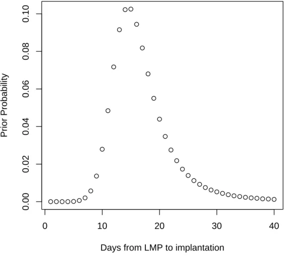
1 Prior probability of conception on a given day of the menstrual cycle, conditional on reaching that day of the cycle. . . 10

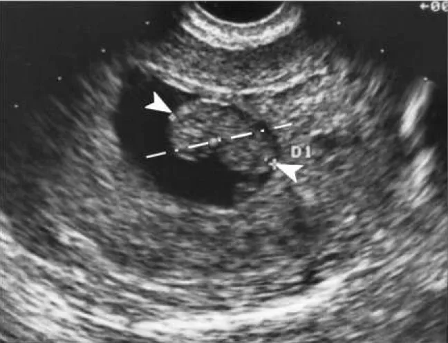
2 Early fetal pole visualization by ultrasound . . . 11

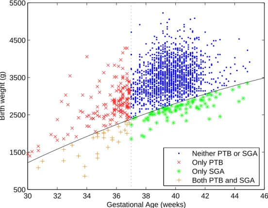
3 Definitions of birth weight, pre-term birth, and small for gestational age. 12

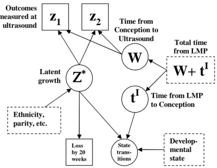
4 Timeline for a subject who has a fetal pole with normal heart rate at time W . . . 56 5 Path diagram illustrating the dependencies in the fetal growth with

un-known initiation times model . . . 57

6 Prior and posterior distributions of the probability of conception on a given day of the menstrual cycle, conditional on reaching that day of the cycle 58

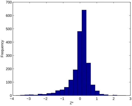
7 Distribution of the posterior means of Z∗

. . . 59

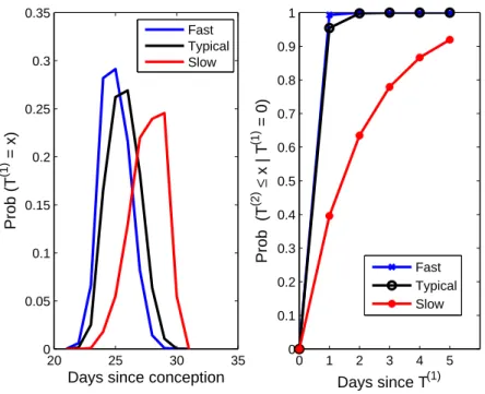
8 Discrete transition rates from a gestational sac to fetal pole (1 → 2, a) and cumulative probability of observing a normal heart rate (2 → 3, b) for three subjects. . . 60

9 Posterior prediction intervals and observed fetal pole lengths for 65 subjects. 61

10 Estimated probability density function for the predominant and residual components of latent immaturity distribution . . . 80

11 Path diagram representing dependencies in fetal development and birth outcomes model . . . 81

12 Probability of being growth restricted at birth for various ranges of early growth restriction . . . 82

13 Empirical and estimated cumulative distribution functions for gestational age at delivery, RFTS data . . . 83

14 Empirical and estimated cumulative distribution functions for birth weight, RFTS data . . . 84

15 Path diagram illustrating the dependencies in the proposed growth restric-tion and latent immaturity model . . . 109

16 Differences in ultrasound measurements of fetal size, blood restriction, and birth weight Z-scores for the restricted and normal latent classes . . . 110

17 Empirical and estimated cumulative distribution functions for gestational age at delivery, PIN data . . . 111

18 Empirical and estimated cumulative distribution functions for birth weight, PIN data . . . 112

(10)

LIST OF ABBREVIATIONS

AC Abdominal circumference

ARS Adaptive rejection sampling

BPD Biparietal diameter

BMI Body mass index

CDF Cumulative distribution function

CI Credible interval

CRL Crown-rump length

EM Expectation-Maximization

FL Femur length

GLM Generalized linear model

GLMM Generalized linear mixed model

HC Head circumference

LMP Last menstrual period

MCMC Markov chain Monte Carlo

MSD Mean (gestational) sac diameter

PI Pulsatility index

PIN Pregnancy, Infection and Nutrition

PTB Pre-term birth

RFTS Right from the Start

(11)

LIST OF ABBREVIATIONS

S/D Systolic-diastolic (ratio)

SAB Spontaneous abortion

SEM Structural equation model

(12)

1 Introduction

Longitudinal data, in which repeated measurements are taken on the same subject over

time, require special statistical methods because observations on the same subject tend to

be correlated. A variety of approaches have been considered to account for the correlation

(Diggle et al. 1994) with the random effects model being one of the most popular methods.

In random effects models, observations on the same subject are assumed to be correlated

due to the effect of some unobservable variables, called the random effects. The random

effects are a type of latent variable, and random effects models are a type of latent

variable method. We will consider several other types of models in which latent variables

are used to account for correlation in longitudinal processes.

Latent variables can be broadly classified into two concepts, latent predictor

vari-ables and latent response varivari-ables. Latent predictors (exogenous latent varivari-ables) are

determined outside of the model and can be related to mis-measured covariates. The

daily average of particulate matter measurement from several monitoring stations is an

example of error-prone realization of a latent true ambient particulate matter

concen-tration predictor variable. Latent responses, also known as endogenous latent variables,

are determined within the model. Latent responses include underlying variables that can

only be measured indirectly through multiple items and are often useful for reducing the

dimensionality of the data. For example, depression is a concept that cannot be

(13)

isolated response on the survey may not be very useful, latent variable methods provide a

natural way of aggregating multiple responses to determine an individual’s latent relative

depression level. In our reproductive health examples, we quantify the latent tendency

of an individual fetus to grow relatively quickly or slowly using information from a first

and second trimester ultrasound and his or her age and weight at delivery.

Latent variables are commonly found in structural equation models (SEMs) used in

the social sciences as a means of quantifying an unobservable concept based on

sev-eral observed variables (Joreskog 1970). SEMs consist of a latent variable model and a

measurement model. The latent variable model describes the association between latent

predictor variables and latent response variables. The second part of the model, the

measurement model, gives the relationship of measured outcomes and predictors with

latent outcomes and latent predictors.

Structural equations models provide a general modeling framework that can be used

for modeling several types of correlated data (Sanchez et al. 2005). Most work in this

area considers SEMs as a model for multivariate normal data, but they can be thought of

in a broader context. Ordinal data are directly incorporated into normal-theory models

by using threshold models. Threshold models are based on the idea that, for example,

the binary observed variableytakes on value one if some underlying continuous variable,

y∗

, is above a threshold value and zero otherwise. The latent y∗

then replaces y in the

SEM (Muthen 1983, 1984). Authors including Sammel et al. (1997) and Dunson (2000)

propose additional extensions that allow for observed outcomes to be in the exponential

family as in the generalized linear model.

(14)

disease. Many diseases can be thought of as moving through several latent health states

with the exact transition times between states unknown. Dunson and Baird (2002)

describe the progression of a chronic condition, uterine fibroids, as progressing from (1)

no disease, (2) preclinical disease, to (3) clinical disease. Information on the current

state as well as several indicators of disease progress can be used to estimate a severity

latent variable. This type of model can provide useful inference on the incidence and

progression of disease using cross-sectional data.

1.1 Reproductive Health Applications

Reproductive and perinatal health spans a broad area of research in maternal and infant

health including infertility, miscarriage, pregnancy complications, birth weight, pre-term

delivery, birth defects, childhood cancer, and child development (Bracken 1984; Kiely

1991). It has been long recognized that events preceding and during pregnancy can

influence the health and well being of both the mother and her child. Researchers have a

dual responsibility to contribute to the practical knowledge that improves health as well

as developing methodology so that we are better equipped to understand future health

problems.

1.1.1 Fetal Growth

During pregnancy, fetal development is traditionally dated from the first day of a woman’s

last reported menstrual period (LMP). The literature intermittently refers to this method

of dating as menstrual age and obstetricians often use the term gestational age

(15)

accurately begin growing at some later time point, which we will refer to as conception.

Conceptional age is also known as fetal age; for consistency, I will only use the terms

gestational age and conceptional age.

In clinical practice, the conceptional age is rarely known so it is estimated based on

the assumption of a midcycle ovulation (conceptional age = gestational age - 14 days).

Estimates of conceptional age are inaccurate due to variability in the follicular phase

distribution, which can vary both among women and within the same woman between

different cycles (Zhou 2006). This variability can be particularly troubling when studying

early fetal development because new structures appear every few days. Several studies,

such as the Early Pregnancy Study (Wilcox et al. 1988), have been conducted to precisely

date the time from LMP to clinical pregnancy. Using urinary biomarkers, Wilcox et al.

(2001) estimated that the probability of conception on a given day of the menstrual

cycle, conditional on reaching that day of the cycle was greatest on day 13 (Figure 1).

The probability is less than 2% for each day before day eight and each day after day 21

of the cycle. Furthermore, the probability of clinical pregnancy on a given day can be

significantly modified by covariates. Wilcox et al. (2001) found the distribution of the

probability of clinical pregnancy by cycle day was more variable with a larger mode for

women with irregular compared to regular cycles.

In our first paper, we are interested in modeling early fetal development as a growth

process with an unknown initiation time. Conception, the unknown initiation time, is

known to occur after the LMP so we estimate the time from LMP to conception.

Individ-ual growth rates are estimated using a latent growth variable that allows individIndivid-uals to

(16)

on growth measured at birth using birth weight and gestational age. In that analysis,

we attempt to identify factors that are related to an individual’s underlying intrauterine

growth rate and a tendency to be born earlier than average. In paper three, we identify

growth restriction using multiple measurements of fetal size and blood flow restriction

collected at two time points during the second trimester. We then examine the

associa-tion between early growth restricassocia-tion and growth restricassocia-tion measured at birth. Papers

one and two are motivated by the Right From the Start (RFTS) study of early pregnancy

(Promislow et al. 2004), and paper three uses information from the Pregnancy, Infection,

and Nutrition (PIN) study (Savitz et al. 1999).

1.1.2 Fetal Development during Pregnancy

Human pregnancies are divided into three trimesters, each normally lasting

approxi-mately 12-14 weeks. In paper one, we are concerned with development within the first

trimester, specifically in the embryonic period which begins with fertilization and lasts

for eight weeks. During the embryonic period, the embryo proceeds through several

im-portant developmental stages. These stages can be defined by the presence or absence

of key features including the gestational sac, yolk sac, fetal pole, and cardiac activity.

Each of these features may be observed by a first trimester ultrasound depending on the

developmental progress of the pregnancy.

The gestational sac is the first structure visualized by sonography and can usually

be seen by the fifth gestational week. The average internal diameter of the gestational

sac is calculated as the mean of the anteroposterior diameter, the transverse diameter,

(17)

(MSD), provides a useful early estimator of age in a normal pregnancy. According to

Filly and Hadlock (2000), the gestational sac can be observed when it reaches 2 to 3 mm

MSD which occurs around 5 gestational weeks. MSDs up to 14 mm are very precise for

predicating gestational age in normal pregnancies, but become less reliable as pregnancy

progresses. According to Filly and Hadlock (2000), the predicted gestational age when

the MSD is 14 mm is 6.5 weeks (95%CI: [6.0, 7.0]). The yolk sac is usually observed

inside the gestational sac during the fifth gestational week. However, the dimensions of

the yolk sac do not significantly improve the ability to predict gestational age, so we do

not consider it in our analysis (Filly and Hadlock 2000).

After the gestational sac and yolk sac, the fetal pole is the next important structure

able to be detected by ultrasound (Figure 2). At this time, the crown-rump length (CRL;

also known as the fetal pole length) becomes the measurement of choice for estimating

gestational age. The fetal pole, without normal cardiac activity, can be visualized when

the CRL is as small as 2 mm, which occurs at 5.7 gestational weeks (95% CI: [5.2, 6.2]).

Normal cardiac activity begins a few days later, by the sixth gestational week (Filly

and Hadlock 2000). Hadlock et al. (1992) evaluated the association between CRL and

gestational age in 416 women with good menstrual dating. They used a fourth order

linear regression model in which CRL was able to predict 98.6% of the variation in the

natural logarithm of gestational age. Their results are similar to predictions reported

by other authors who often used only linear or quadratic CRL effects. An advantage of

the Hadlock study is that it included a relatively large sample with a greater range of

CRL measurements (from 2 mm to 120 mm) than other studies. The additional small

(18)

Researchers have conducted studies to determine if gestational sac diameters or crown

rump lengths measured by an early ultrasound are indicative of early pregnancy loss.

Nyberg et al. (1987) collected data on 83 women who had two sonograms performed

during the first trimester of pregnancy. The subjects were referred for a second ultrasound

due to bleeding or pelvic pain (64 cases) or to confirm the pregnancy (19 cases). They

found that gestational sac growth was significantly slower in women who eventually

had abnormal pregnancies compared to women with normal pregnancies. However, in

evaluating 254 viable singleton pregnancies, Brizot et al. (2001) were not able to confirm

this result. Mantoni and Pedersen (1982) examined 67 patients with threatened abortion

with regular, known menstrual cycles. They found that the crown rump length of these

fetuses was smaller than expected based on their gestational age. There was also some

evidence that the fetuses that eventually aborted had on average smaller crown rump

lengths. Again, Brizot et al. (2001) could not replicate this result. Rather than consider

gestational sac diameters and fetal pole lengths directly, we conceptualize that they are

indicators of underlying fetal growth. In paper one, we estimate an early fetal growth

latent variable and examine its association with the risk of pregnancy loss.

1.1.3 Birth Weight

Birth weight is an important predictor of perinatal, neonatal, and postnatal outcomes

(Shan and Ohlsson 2002). Poor growth during the intrauterine period is associated with

increased risk of perinatal and infant morbidity and mortality. Many epidemiological

studies have been conducted to elucidate some of the determinants of birth weight.

(19)

of low birth weight, and alcohol use are generally accepted as having a strong association.

Other studies have found various environmental and occupational exposures, caffeine use,

uterine fibroids, and stress may be associated with growth and require further research

(Shan and Ohlsson 2002).

Zhang and Bowes (1995) attempted to create a standard for identifying small for

gestational age (SGA) infants stratified on race, gender, and parity. Gestational age

was calculated using LMP data for more than 95% of all subjects, but in some cases a

clinician-based adjustment was needed to correct inaccurate LMPs. The authors do not

report statistical test results indicating if they found significantly different growth curves

by race, gender, or parity. However, they do provide graphs that indicate these covariates

may be associated with growth as measured by birth weight between 25 and 42 weeks

gestation. We will examine the association of race, gender, and parity with growth rate

during the first trimester.

Weight at birth is a function of both the amount of time from conception to birth and

the intrauterine growth rate of a fetus. Low birth weight can result from slow intrauterine

growth, early conceptual age, or a combination of the two. Figure 3 plots birth weight

versus gestational age to help describe the different type of outcomes that could be

observed in a population of newborns. Most newborns are normal age and weight, but

some will be born below the 10th percentile of weight for a given gestational age (small

for gestational age, SGA) and others may be born before the 37th week of gestation

(pre-term birth). Some newborns will be both pre-(pre-term and SGA. In papers two and three,

we capture the correlation between birth weight and gestational age using an immaturity

(20)

approach also allows us to identify a latent class of subjects with early gestational age

and low weight. In reproductive health, epidemiologists refer to these types of subjects

as belonging to the “residual” distribution (Wilcox et al. 2001), and they are of special

importance because they are at increased risk for mortality and other forms of morbidity

(Buekens et al. 2000). We attempt to find covariates that are associated with belonging

to the residual distribution.

1.2 Other Applications

Our research is motivated by an application in reproductive health, but the methods

we propose can be applied to other areas as well. We explain models using examples

from other disciplines throughout this dissertation, and provide a brief overview of the

most common applications here. SEMs are primarily found in the social sciences (Bollen

1989), and Sanchez et al. (2005) advocates their use in environmental epidemiology. In

the statistics literature, reproductive toxicology has been used to motivate both

multi-state growth models (Sternberg and Satten 1999) as well as mixed continuous and

dis-crete outcomes (Catalano and Ryan 1992). Other examples of multistate models come

from AIDS research (DeGruttola and Lagakos 1989), the development of uterine fibroids

(21)

0 10 20 30 40

0.00

0.02

0.04

0.06

0.08

0.10

Days from LMP to implantation

Prior Probability

Figure 1: Prior probability of conception on a given day of the menstrual cycle,

(22)

Figure 2: Early fetal pole visualization by ultrasound. The pole is indicated by the two

(23)

30 32 34 36 38 40 42 44 46 500

1500 2500 3500 4500 5500

Gestational Age (weeks)

Birth weight (g)

Neither PTB or SGA Only PTB

Only SGA

Both PTB and SGA

(24)

2 Latent Variable Methods for Longitudinal Data

Latent variable methods can capture many statistical concepts including random effects,

missing data, sources of variation in hierarchical data, finite mixtures, latent classes, and

clusters (Muthen 2002; Sanchez et al. 2005). In this section, we review several types of

latent variable methods for longitudinal data.

2.1 Random Effects Models

Random effects models are commonly used for longitudinal data in which repeated or

otherwise correlated measurements are taken on the same subject. The linear random

effects model as proposed by Laird and Ware (1982) is specified by

yi =Xiβ+Zibi+i, i= 1, ..., n (2.1)

where y_i is ni ×1, Xi is an ni × p matrix of fixed predictors, β is a p×1 vector of

fixed effects, Zi a ni×q vectors of covariates for the q×1 vector of random effects bi,

and i is an ni ×1 vector of random errors. It is standard to assume thati and bi are

independent and both normally distributed

bi ∼Nq(0,D) (2.2)

and

(25)

so that, marginally,

yi|β,Ri,D∼Nni(Xiβ,Ri+Z 0

iDZi) (2.4)

Random effects models can also be specified for non-continuous outcomes. The

gen-eralized linear model (GLM) extends the methods of regression analysis to outcome

vari-ables that follow other distributions in the exponential family (McCullagh and Nelder

1989). For example, the binomial distribution is often used for binary outcomes and

the Poisson distribution for counts. The generalized linear mixed model (GLMM) is the

GLM generalization of the linear random effects model and is specified by Diggle et al.

(1994) as

• Given bi, the responses y_i are mutually independent for each i and follow a GLM

with density f(yij|bi) = exp[{(yijθij − ψ(θij))}/φ +c(yij, φ)]. The conditional

moments µij = E(yij|bi) = ψ0(θij) and vij = Var(yij|bi) = ψ00(θij)φ, satisfy

h(µij) =x0ijβ+z 0

ijbi and vij =v(µij)φ whereh andv are known link and variance

functions, respectively, and zij is a subset of xij

• The random effectsbi are mutually independent with a common underlying

distri-bution,F

Frequentist likelihood-based estimation of the GLMM can be computationally difficult

because high dimensional integrals are needed to evaluate the marginal likelihood

(Bres-low and Clayton 1993). In contrast, likelihood-based Bayesian methods are relatively

straightforward to carry out using the Gibbs sampler because we can sample parameters

conditionally on the random effects (Gelfand and Smith 1990).

(26)

heterogeneity across individuals that can be represented in their regression coefficients.

Observations on the same individual are correlated due to sharing some unobservable

variables, bi. A model of this type is sometimes referred to as a kind of latent variable

model (Diggle et al. 1994) with the unobserved random effects being considered latent

variables.

2.2 Latent Class Trajectory Models

Growth models, which model the changes in individuals over time, are one traditional

application for random effects models. A growth model that allows for a quadratic effect

of time for subject i measurement j at age tij could be specified using the notation of

Laird and Ware by

yij = (β0+b0i) + (β1+b1i)tij+ (β2+b2i)t2ij+ij (2.5)

where bi ∼ N(0,D) and i ∼ i.i.d.Nni(0,Ini). An equivalent representation of this

model in terms of subject-specific latent variables η0i for the intercept, η1i for the linear

effect and η2i for the quadratic effect is

yij =η0i+tijη1i+t2ijη2i+ij (2.6)

where ηi ∼N([β0, β1, β2]0,D) and i ∼i.i.d.Nni(0,Ini).

It may be of interest how the shape of an individual growth trajectory, as measured

by the latent variables, is related to some outcome measure. For example, Muthen

and Shedden (1999) are interested in the association between the shape of an alcohol use

trajectory from ages 18-25 and the risk of alcohol dependence at age 30. Directly relating

(27)

because the meaning of a given η_i coefficient depends on the values of the other η_i

coefficients. For example, a subject with a positive linear slope (η1i > 0) could have

decreasing dependence over time (ifηi2 <0), a purely linear increase over time (ifηi2 = 0),

or increase very rapidly over time (ifηi2 >0). A better option is a latent class trajectory

model.

A latent class model summarizes shared features of the η coefficients using an

un-derlying categorical variable. Specifically, the mi-dimensional ηi are related to the

K-dimensional latent categories ci and p-dimensional covariates xi using

ηi =Aci+Γηxi+ζ, ζi ∼Nmi(0,Σ) (2.7)

with conforming parameter matrices A(mi×K) and Γη(mi×p). The latent categorical

variable, ci = (ci1, . . . , ciK) follows a multinomial distribution with cik = 1 if individual

i falls in class k and zero otherwise. A r-dimensional vector of observed dichotomous

outcome variablesuican then be related to the latent categories using a logistic regression

model

logit (Pr(uij= 1|ci)) =Λu,jci (2.8)

where eachΛu,jis an 1×K parameter matrix,j = 1, . . . , K. To complete the specification

of the model, Muthen and Shedden (1999) allow the categorical latent variablescto be

re-lated to covariatesxusing a multinomial logit model for unordered polytomous responses.

Defining πik = Pr(cik = 1|xi) and the logit(πi) = (log [πi1/πiK], . . . ,log [πi,K−1/πiK]),

logit(πi) = αc+Γcxi (2.9)

(28)

this specification, the conditional distributions of y and u given x are influenced by

parameters that vary across the categories of c.

Several recent articles have built on these results. Guo et al. (2006) extend the latent

class regression model so that it can include regression on latent predictors. Miglioretti

(2003) discusses additional challenges that arise when the longitudinal measurements are

mixtures of continuous, binary, and count data. Lin et al. (2000) use a latent class model

to uncover subpopulation structure for both biomarker trajectories and the probability

of disease outcome in highly unbalanced longitudinal data.

2.3 Structural Equation Models

SEMs are a flexible class of models originally proposed by Joreskog (1970) that allow

modeling of both multivariate data and multiple, closely related predictors. The SEMs

described in the book by Bollen (1989) incorporate a measurement model and a latent

variable model for multivariate normal data. Using the notation of Bollen, the latent

variable model is

η=Bη+Γξ+ζ, ζ ∼Nm(0,Σ) (2.10)

where η is and m×1 vector of latent responses, B an m×m coefficient matrix, and ξ

are latent predictor variables (n×1) with coefficient matrixΓ (m×n). The latent class

model given in (2.7) is a special case of (2.10) whereB =0,Γ= [A;Γη], andξ = [ci;xi].

The measurement model is then given by

y=Λyη+, ∼Np(0,Σy) (2.11)

(29)

The vectorsy(p×1) andx(q×1) are observed variables with coefficient matrices, referred

to as “factor loadings” in SEMs, Λy(p×m) and Λx(q×n) and with errors (p×1) and

δ(q×1), respectively. Identifiability is an important consideration in SEMs, and is often

accomplished by constraining covariance matrices to be diagonal, factor loading matrices

to be equal to one, and/or the variance of the latent variables to be unity (Bollen 1989).

Some researchers have given particular attention to models that contain observed

variables that are multiple indicators and multiple causes of a single latent response

variable (MIMIC) as we have in the early pregnancy example (Joreskog and Goldberger

1975). In the MIMIC model, Λy = Iq and the latent predictor variables are observed

without error (x=ξ) so thatη is a stochastic function ofxwith coefficients Γand error

component ζ1:

η =Γx+ζ1, ζ1 ∼N(0, σ2). (2.13)

We say thatηis affected by one or morexvariables and it is associated with one or more

y variables such that

y =Λyη+ (2.14)

with errors and factor loadings Λy. This model will be identifiable if there are at least

two y variables, at least one x, and η is provided a scale by either fixing the variance of

ζ1 or a factor loading term (e.g. ζ1 ∼ N(0,1) or λ1 = 1). Identifiability of these models

as well as more general models with multiple latent variables is often a concern and is

discussed by Stapelton (1977), Robinson (1974), and Bollen (1989) among others.

Mixed effects models are closely related to SEMs where the random effects are latent

(30)

sampling unit. While conceptually similar, there are some important differences in how

they specify the mean and covariance models. To clarify the differences, consider a

p-dimensional vector of responses y_i = [yi1, yi2, . . . , yip]0 that has a linear relationship with

dose. A linear random effects model as in (2.1) could be fit

yij =β0j+β1j ∗dosei+bi1+bi2∗dosei+ij, ij ∼N(0, σ2) (2.15)

The same data could be analyzed with the SEM

yij = µj +λj∗ηi+ij, ij ∼N(0, σ2j) (2.16)

ηi = γ1∗dosei+δi, δi ∼N(0,1) (2.17)

The SEM estimates additional factor loading terms λj(λj ≥ 0) that multiply the latent

variable to allow for a non-exchangeable correlation structure as well as differences in

scale between the measured outcomes (Dunson 2006b). The correlation structure for the

random effects model is allowed to vary by dose, but for the control group (dose = 0)

simplifies to a compound-symmetric structure. In the SEM, the correlation between yij

and yij0 is given by

corr(yij, yij0) =

λjλj0

q λ2

j +σ2j

q λ2

j0+σ_j20

(2.18)

which can differ for different sets of outcomesj andj0

. A potentially important advantage

to the random effects model is that it allows heterogeneity in the regression coefficients

for dose across different responses. Models that combine the benefits of random effects

models and SEMs are an area of current research (Dunson 2006b). Lin et al. (2000)

and Roy et al. (2003) consider other approaches for allowing differences in scale when

(31)

While Bollen considers SEMs as models for multivariate normal data, they can be

considered in a wider context. Longitudinal data can be measured on binary scale,

cat-egorical (ordinal or nominal) scale, metric scale (discrete or continuous), or in various

combinations. Other researchers have considered latent variable models which allow

measured and latent variables to have a broader class of distributions. Dunson (2000),

Sammel et al. (1997), and Moustaki and Knott (2000) consider distributions in the

expo-nential family for modeling variables that are collected on a variety of scales. In papers

two and three, we relax the normality assumption and consider options including a latent

class model in which the latent variable follows a mixture distribution.

2.4 Bayesian Structural Equation Models

The majority of literature on SEMs using latent variables is frequentist in nature, but

Bayesian approaches have been proposed by several authors. There is a long history for

Bayesian analysis of factor models, which are a special case of SEMs, in the psychometrics

literature (Ansari and Jedidi 2000; Lee 1981; Martin and McDonald 1975). Early work

on more general SEMs was done by Lee (1992) and Bauwens (1984).

There are several important differences between a Bayesian and frequentist approach

to latent variable models. While frequentists usually assume normal distributions for

latent variables, Bayesians must specify prior distributions for all unknown parameters in

both the latent variable and measurement models. The priors allow for information from

previous studies or theory to inform about the nature of the structural relationships, or,

in the absence of such information, vague priors can be used. Computationally, Bayesian

(32)

computationally expensive but provide exact posterior distributions for functions of any

unknown parameters.

A Bayesian perspective allows us to estimate the posterior distribution of latent

vari-ables as well as parameters without making asymptotic assumptions. As pointed out by

Palomo et al. (2007), estimating the joint posterior of latent variables has several

advan-tages over a frequentist approach. For one, we can obtain point and interval estimate

of factor scores for each individual in the study. We can then compare different factor

scores among individuals (through posterior probabilities that, for example, one score is

higher than another) and if an individual’s factor score changes over time. We can also

identify outlying individuals who are at the tail of the distribution.

A downside of a Bayesian approach to SEMs is that high autocorrelations can lead

to slow convergence of the Gibbs sampler. It may take several hours of sampling until

the Monte Carlo error in sampling is negligible. Recent articles have focused on MCMC

methods to implement Bayesian analysis in complex cases including non-linear systems

(Arminger 1998; Lee and Song 2004) and multi-level data (Dunson 2000; Song and Lee

2004). We discuss computational issues in more detail in section 3.

2.5 Multistate Models

A multistate process is a stochastic process that can take on a finite number of states K

where each state describes the current condition (Jewell 2005; Kalbfleisch and Prentice

2002). In a general form where we allow time to be continuous, we define Y(t) to be the

state of the process at time t, Y(t)∈ {1,2, . . . , K} and t ≥0. A Markov process is the

(33)

with no covariates, the transition rate from state i toj for an individual who is in state

i at time t−

is given by

dΛij(t) = P

Y(t−

+dt) =j|Y(u),0≤u < t, Y(t−

) =i

= P

Y(t−

+dt) =j|Y(t−

) = i

for all Y(u),0≤u < t, j 6=i. The Markov assumption is that the process is memoryless

in that only the current occupied state is need to specify the transition rates. Transition

rates are allowed to depend on t, the amount of time since the beginning of the study.

In a general multistate model, subjects are allowed to transition from any state k to

another state k0

. Multistate growth models impose some restrictions on the multistate

model. For one, growth models are unidirectional. That is, state transitions occur in a

distinct order, only moving from statekto statek+1,k = 1, . . . , K−1. Also, all subjects

begin at the same initial state, k = 1. Traditional survival analysis, where subjects only

move from “at risk” to “failed” states is a simple example of a unidirectional multistate

process with K = 2.

In a regular Markov model, we are able to observe the states directly so that the state

transition probabilities are the only parameters of interest. In a hidden Markov model

the complete state history of a multistate processY(t) is not available at every time point

t, but variables that are influenced by the state are observed. The influencing variables

can be linked to underlying latent progress variables that are indicative of the waiting

time spent in a state (Dunson and Baird 2002). In a longitudinal study, the state may be

observed at several time points for each subject but the exact transition times are only

(34)

only available at one time point. We are concerned with the cross-sectional case where

state transition times are interval censored and developmental progress covariates are

measured once for each subject.

We consider multistate growth models where the moment the process begins, called

the initiation time, is not known. The earliest approaches for multistate models with

unknown initiation times relied on the restrictive Markov assumption (Kalbfleisch and

Lawless 1985), which is not appropriate in our application. Semi-Markov models for

fitting interval censored data with unknown initiation times (Satten and Sternberg 1999)

have been developed that allow transition rates to depend on the amount of time spent

in the state. In the fetal growth example, we consider the LMP date to be a known,

pre-initiation time and conception the unknown pre-initiation time. With this fixed time scale,

it would also be possible to use the semi-Markov methods of DeGruttola and Lagakos

(1989) or Sternberg and Satten (1999) by considering the pre-initiation time to be the

first stage in the network. If the waiting times in different states are independent, then

the semi-Markov assumption will hold. We avoid the semi-Markov assumption and allow

individual transition rates between states to be influenced by a subject-specific latent

(35)

3 Computation

When proposing structural equation models, it is particularly important to consider

which parameters in the model are identifiable and which must be constrained. In many

cases, the marginal likelihood can be examined to determine how the data informs about

each parameter. In a Bayesian analysis, fitting MCMC models can be somewhat of an art

form so that alternative strategies may be needed to achieve dependable results (Gelfand

and Sahu 1999). For example, including parameters that are non-identifiable, with

ap-propriately vague priors, can help improve convergence. In this section, we first provide a

brief introduction to Bayesian methods. We then define identifiability and Bayesian

iden-tifiability and explain one way in which including non-identifiable parameters in a model

can improve computational performance while introducing a more general class of

con-ditionally conjugate priors. This section is concluded by describing a data augmentation

algorithm useful for fitting probit and multivariate probit models.

3.1 Bayesian Methods for Data Analysis

Bayesian methods are a useful tool for the applied statistician with applications in a

wide range of areas due to the development of MCMC methods and the corresponding

expansion of computing power. The details of a Bayesian approach to data analysis

(Carlin and Louis 2000; Gelman et al. 2004) are well beyond the scope of this dissertation.

(36)

following sections.

The flexibility of the Bayesian framework allows it to deal with very complex

analyt-ical problems while using relatively simple conceptual methods. Bayesian methods are

based on estimating the posterior distribution of p parameters θ given the data x and

hyperparameters η, f(θ|x,η). Using Bayes’ Theorem,

f(θ|x,η)∝L(θ)π(θ|η) (3.1)

whereL(θ) =f(x,θ|η) represents the likelihood andπ(θ|η) the prior distribution onθ.

Inference is then based on the posterior distribution of parameters θi.

It is often difficult to directly calculate the complete joint posterior distribution,

f(θ|x,η), when p is not small. Gibbs sampling (Gelfand and Smith 1990; Geman and

Geman 1984) is a commonly used MCMC method to draw elements ofθindividually or in

small groups. The Gibbs sampler generates values from the joint posterior distribution by

iteratively drawing samples from the complete conditional distributions f(θi|θj,x,η, i6=

j) for each i = 1, . . . , p0

≤ p. After sufficient iterations, draws from the individual

complete conditionals will eventually converge to being draws from the desired posterior

distributionf(θ|x,η). When conjugate priors are chosen, it is often easy to sample from

the complete conditionals because they are of known forms. For complete conditionals

of unknown form, sampling can be done using the Metropolis-Hastings Algorithm (Chib

and Greenberg 1995; Hastings 1970) with proposal densities generated from adaptive

rejection samplings (ARS; Gilks and Wild 1992) or ARMS (ARS with a metropolis step;

Gilks et al. 1995. Iterations continue until the parameters are judged to converge by a

(37)

3.2 Identifiability

A parameter θ is (frequentist) identifiable by observations of a random vector y if

dis-tinct values for θ yield distinct distributions for y (Basu 1983). Bayesian identifiability

(Dawid 1979) focuses on the posterior distribution and is concerned with whether the

data and prior provide information about the parameters. Situations can arise where

parameters are not frequentist identifiable, but can identified in a Bayesian analysis that

uses informative priors. In these cases, parameters that are only Bayesian identifiable

need to be recognized and interpreted appropriately.

Specifying a proper prior ensures a proper posterior. However, improper priors are

often used to reflect ignorance of parameters or for mathematical convenience. Gelfand

and Sahu (1999) explore the use of improper priors for the generalized linear model and

developed the following theorem:

Consider the Gaussian linear model y = Xβ + with Xn×p, βp×1, with

rank(X) = r < p and ∼ N(0, σ2_{I). Suppose that the prior} _{f(β, σ}2_{) takes}

the form f(β)f(σ2_{), where} _f_{(β) =}_f_{(γ), a proper prior on} _γ _{= Ωβ} _{with Ωβ}

estimable. Then f(β, σ2_{|y) is improper.}

A proper prior will need to be specified on some non-estimable parameters for the

posterior to be proper. In the frequentist setting, this is usually accomplished by

con-straining certain parameters to be equal to some value (usually 0). Gelfand and Sahu

(1999) give a logistic growth curve example to illustrate that this is not an ideal

solu-tion when performing Gibbs sampling. They show that placing non-informative (but

(38)

signif-icantly decrease the autocorrelation of estimable parameters. The worst convergence of

the Markov chain is attained by imposing constraints. Gelman et al. (2003) also notes

for the generalized linear model more diffuse working prior densities improves mixing.

Recent papers on parameter expansion elaborate on these ideas.

3.3 Parameter Expansion

Parameter expansion adds new parameters that are not identifiable to a model. An

example is replacing a parameter θ by a product φψ so that inference can be obtained

only about the product and not the individual parameters. This technique has been

used to improve the convergence rate of the EM algorithm by Liu et al. (1998) in a

non-Bayesian setting. Gelman (Gelman 2004; Gelman et al. 2003) uses parameter expansion

as a computational aid within a Gibbs sampling framework, which we will find more

useful.

Gelman considers the following hierarchical model expressed as a regression with

coefficients in M batches.

y=

M

X

m=1

X(m)_β(m)_{+ error}

whereX(m)_{is the}_{mth submatrix of predictors and}_β(m)_{is the}_{mth subvector of regression}

coefficients. The Jm coefficients in each subvector β(m) have an exchangeable N(0, σm2)

prior distribution for j = 1, . . . , Jm. He uses this general notation to allow for several

different types of models. We are interested in a mixed effects model where, for the fixed

effects, σm =∞and, for the random effects, σm is estimated from the data.

This hierarchical model can become stuck when σm happens to be near 0. In the

updating stage of the Gibbs sampler, β(m) _{will be shrunk to 0, at the next update} _σ

(39)

will be near 0, and so on. Simulations show that it can take considerable time for the

Gibbs sampler to escape this situation (Gelman et al. 2003).

Gelman (2004) advocates using the following parameter-expanded model where each

component of the regression model is multiplied by a new parameter, α∗

m. Let the old

model be

y=

M

X

m=1

X(m)β(m)+ error

and the new, expanded model be

y = M X m=1 α∗ mX

(m)_β∗(m)_{+ error}

The estimable function |α∗ m|σ

∗

m in the new model maps to σm in the old model and

α∗ mβ

∗(m)

j from the new model maps toβ

(m)

j from the old model. The individual parameters

α∗ m, β

∗(m)

j , andσ ∗

m are not frequentist identifiable, but if proper priors are specified, they

will be Bayesian identifiable.

Gelman (2006) examines different choices for prior distributions in the hierarchical

model. He expands the family of conditionally-conjugate prior distributions by applying

a redundant multiplicative reparameterization to the general hierarchical model:

yij ∼ N(µ+ξηj, σy2)

ηj ∼ N(0, ση2)

There is an implicitly conditionally conjugate prior distribution on the random effects

standard deviation, σα = |ξ|ση. Using the usual conjugate priors for ξ (normal) and ση2

(inverse-gamma), σα has the distribution of the absolute value of a noncentral-t

(40)

special case of the folded non-central t, the half-t distribution. This half-t is appealing

because the distribution of ξ will be symmetric about 0, however the half-tfamily is not

conditionally conjugate.

In summary, Gelman’s findings and advice include:

• Start with a noninformative uniform prior density on the standard deviation σα

• For a non-informative but proper density, try a half-normal centered at 0, ξ ∼

N(0,1002₎

• Avoid the usual inv-gamma(, ) priors on σ2

α especially when small values of σα

are possible. Inference is very sensitive to and the prior distribution is not

non-informative as desired.

• To restrict σα from large values, use a half-t family

We found these suggestions particularly helpful in the early fetal growth analysis.

Con-vergence rates were improved while using a less informative prior than the usual gamma

prior on precision parameters.

3.4 Data Augmentation

Data augmentation is a general scheme in which the observed data are enhanced so as

to make it easier to analyze. Dempster et al. (1977) popularized the method with their

paper on the EM algorithm for maximizing a likelihood function, but their approach

was not called “data augmentation” until Tanner and Wong (1987). From a Bayesian

(41)

observed data to calculate the posterior distribution of the parameters of interest (van

Dyk and Meng 2001). For observed binary data, data augmentation postulates the

existence of an underlying continuous variable such that the event is observed to occur if

the continuous variable is above some threshold value. Using this idea, we can use latent

variables to facilitate model computation for categorical outcomes.

The data augmentation algorithm outlined by Albert and Chib (1993) connects a

pro-bit regression model on an observed dichotomous outcome with a normal linear regression

model on a continuous latent outcome. Their algorithm involves sampling latent outcome

variables from the truncated normal distribution, with the truncation conditional on the

observed dichotomous outcome variable. Lety1, . . . , ynbe the observed dichotomous

out-come on subject i and y∗

i the underlying latent response, where y ∗

i are i.i.d. N(x 0 iβ,1).

Define yi = 1 if yi∗ > 0 and yi = 0 otherwise so that the yi are independent Bernoulli

random variables with P r(yi = 1) = Φ(x0iβ) where Φ(·) is the standard normal

cumula-tive distribution function. The complete conditional distribution of the latent y∗

i is then

given by

y∗

i|yi,xi,β∼

      

N1(x0iβ,1)I(y ∗

i >0) if yi = 1

N1(x0iβ,1)I(y ∗

i <0) if yi = 0

(3.2)

With a conjugate prior specification for β, Gibbs sampling can then be used to sample

from the posterior distribution of β using well known linear regression results. To

sim-plify subsequent notation, the general truncated normal distribution as given in (3.2) with

σ2 _{= 1 will be specified as}_{T N}₍_x0

iβ, σ2, yi). The underlying latent normal approach can

naturally be extended to the multinomial probit model (McCulloch and Rossi 1994) for

(42)

Green-berg 1998) for multivariate binary correlated outcomes.

3.5 Multivariate Probit Models

Chib and Greenberg (1998) detail an approach for modeling multivariate correlated

bi-nary data that is a natural extension of the univariate probit model framework. Let yij

be a binary response for theith observation unit andjth variable,j = 1, . . . , p. Chib and

Greenberg (1998) postulates the existence of an underlying multivariate normal random

vector

y∗

i ∼Np(Xβ,Σ) (3.3)

such that yij = I(yij∗ > 0) and Σ is a correlation matrix for identifiability. We can

then extend this representation for joint modeling of continuous and binary correlated

outcomes. Let zi1 be a p1-dimensional vector of observed normal continuous response

and zi2 a p2-dimensional vector of binary responses with underlying responses z∗i2. The

joint distribution of zi1 and z∗i2 is given by

    zi1 z∗ i2    

∼Np1+p2     Xβ,    

Σ11 Σ12

Σ21 Σ22         (3.4)

where the diagonal elements of Σ₂₂ are fixed at one for identifiability. The problem is

now reduced to modeling normally distributed correlated data using observed and latent

continuous random variables.

While the relatively direct probit model framework for analyzing mixed continuous

and discrete outcomes is conceptually appealing, it can be computationally demanding.

In a Bayesian analysis, high autocorrelations within parameters and cross correlations

(43)

number of approaches have been suggested to improve mixing and the convergence rates

of longitudinal models and the multivariate probit model that we may be able to adapt

for modeling mixed continuous and discrete outcomes.

Gelfand et al. (1995) presents hierarchical centering reparamaterizations that often

have improved convergence for a broad class of normal linear mixed models. Hierarchical

centering can be explained by considering the simple random effects model yij = µ+

bi1 +ij, where bi1 ∼ N(0, σb2) and ij ∼ N(0, σe2) i.i.d for each subject i and repeated

measurej. In order to create a better-behaved posterior surface, a second level hierarchy

is introduced by defining ηi = µ+ bi1 such that ηi|µ ∼ N(µ, σ2b). The hierarchical

centering transformation can break the high posterior correlations among parameters

that commonly occur in random effects models and greatly improve convergence of the

Gibbs sampler.

The benefits of blocking, which involves updating parameters in groups, in

hierarchi-cal longitudinal models are advocated by Chib and Carlin (1999). They also specifihierarchi-cally

consider longitudinal binary probit models of the form Pr (yij = 1|bi) = Φ(x0ijβ+z 0 ijbi)

where Φ is the standard normal CDF and bi ∼ Nq(0,D). Then the conditional

distri-bution of the latent outcome, yij =I(yij∗ >0), is given by y ∗

ij|bi ∼N(x 0

ijβ+z 0

ijbi,1). A

simple algorithm for sampling from the joint posterior that updates parameters one at a

time will include sampling (1) β|y∗

,b,D and (2) y∗

ij|yij,β,b,D as well as (3) b|y∗,β, D

and (4) D|b. Chib and Carlin (1999) refine this algorithm by marginalizing the

dis-tribution of y∗

i over the random effects so that y ∗

i ∼ Nni(Xiβ, Ini+ZiDZ 0

i). Steps

(1) and (2) of the simple algorithm are blocked so that we sample both β and y∗ i from

[β,y∗

i|y,D] by sampling (a) β|y,y ∗

,D and (b) y∗

(44)

approach and some similar variations significantly reduce autocorrelations for β, but are

less effective on improving convergence for the random effect variance,D.

Imai and Van Dyk (2005) and Nobile (1998) propose methods for improving the

convergence of the multinomial probit model. They realize that one of the reasons for

the poor convergence of probit models is the variance of the latent response variable is not

identifiable and is fixed at one by convention. Imai and Van Dyk (2005) introduce a new

latent variable ˜y∗ i =αy

∗

i so that ˜y ∗

i|β, α, yi ∼T N(αXiβ, α2,y). An inverse gamma prior

is specified for α2 _{and it is included as part of the Gibbs sampling algorithm. Nobile}

(1998) develops a hybrid Markov chain in which a Metropolis step is performed after

each cycle of the Gibbs sampler to change the scale of the current state. Both methods

improve the computational efficiency of simulated data, with the more recent paper of

(45)

4 Bayesian Modeling of Embryonic Growth using

Latent Variables

4.1 Abstract

In a growth model, individuals move progressively through a series of states where each

state is indicative of their developmental status. Interest lies in estimating the rate of

progression through each state while incorporating covariates that might affect the

tran-sition rates. We develop a Bayesian discrete time multistate growth model for inference

from cross-sectional data with unknown initiation times. For each subject, data are

col-lected at only one time point at which we observe the state as well as covariates that

measure developmental progress. We link the developmental progress variables to an

underlying latent growth variable that can affect the transition rates. We also examine

the association between latent growth and the probability of future events. We use a

Markov chain Monte Carlo algorithm for posterior computation and apply our methods

to a novel study of embryonic growth and pregnancy loss in which we were able to find

evidence in favor of a previously hypothesized but unproven association between slow

(46)

4.2 Introduction

Fetal growth is important both clinically and in epidemiologic studies relating growth

to later pregnancy and developmental outcomes. To date, large cohort studies have

re-lied on the last menstrual period (LMP) and onset of bleeding to determine the time

of miscarriage. This approach is centrally flawed because it ignores the developmental

state of the fetus prior to the loss. Development may stop days to weeks prior to the

onset of bleeding so that, for example, a loss classified as a miscarriage in the 10th week

of gestation may have been the loss of an appropriately-grown 10 week fetus, or a fetus

with development arrested at 7 weeks. Coupling cross-sectional ultrasound information

with the ability to estimate growth provides an opportunity to estimate probable

devel-opmental state prior to miscarriage. This can help researchers more accurately identify

which insults must have occurred prior to the pregnancy loss and rule out exposures that

occur after development arrest but before the onset of bleeding.

Another complication in determining the miscarriage date is uncertainty in pregnancy

dating. After the occurrence of a positive pregnancy test, time of conception is

tradi-tionally dated as two weeks after the LMP. Such dating is notoriously imprecise due to

variation in follicular phase length, the time between menses and ovulation, and, in rarer

cases, missed menses (Kramer et al. 1988; Savitz et al. 2002). However, the distribution

of the follicular phase length has been well characterized (Wilcox et al. 2001) and can

be used to obtain more realistic estimates of the conception time. With these difficulties

in mind, our goal in the early pregnancy example analysis is two-fold: (1) to determine

(47)

varia-tion in growth exists, to determine if growth is associated with the probability of future

pregnancy loss. In particular, if (2) holds the current practice of using ultrasound dating

in early pregnancy loss studies may need to be re-evaluated.

This vexing problem can be posed statistically using a latent multistate growth process

with unknown initiation time. In a multistate model the current condition of a subject

is summarized by assignment to one of a finite number of K states (Jewell 2005). A

growth model assumes that all subjects begin at the same initial state and advance

unidirectionally through subsequent states. That is, all subjects progress in order from

state k to k+ 1, k = 1, . . . , K−1 without skipping any states or regressing to previous

states. This article focuses on the problem of estimating such models using cross-sectional

data in which transition times are not observed. For each subject, we have information

at one time point on the current state as well as measurements of developmental progress

that are surrogates of the amount of time spent in a state. Also, the moment the growth

process begins, referred to as the initiation time, is not known, though some time point

before initiation is known.

Multistate growth models with interval censored transition times appear in several

applications. Often the initiation time is also unknown but not considered in the analysis.

One example involves studying tumor growth in mice. Typically, a mouse is exposed to a

carcinogenic compound and a tumor may develop some time following the exposure. At a

later date, the mouse is sacrificed to determine how far the tumor has progressed (Albert

and Shih 2003; Dewanji and Kalbfleisch 1986; Ryan and Orav 1988). In these studies,

the investigators analyze time from exposure rather than time from tumor initiation. We

(48)

in our application, failing to account for the unknown initiation time can have a large

impact on the analysis. Other examples of multistate models include AIDS progression

(DeGruttola and Lagakos 1989), breast cancer (Duffy et al. 1995), and the development

of uterine fibroids (Dunson and Baird 2002). Our research is motivated by the Right

from the Start (RFTS) study of embryonic development.

RFTS is a prospective cohort study that identified women who were planning to

conceive or in early pregnancy (Promislow et al. 2004). Investigators enrolled women

when they had a positive pregnancy test, and then promptly provided an early first

trimester ultrasound. At the time of the ultrasound, each fetus was assigned to one of

three states based on the presence or absence of important developmental features: (1)

only gestational sac present, (2) fetal pole present without regular cardiac activity, and

(3) fetal pole with normal cardiac activity. Lack of cardiac activity is a natural state of

development that every fetus experiences for hours to days while the heart forms, becomes

detectable by ultrasound, and before a heart rate is established. It is not necessarily

indicative of a problem pregnancy. The ultrasound also provides two measurements of

developmental progress, the mean gestational sac diameter and fetal pole length. Both of

these covariates have been studied extensively and found to be strongly associated with

time since LMP (Filly and Hadlock 2000; Hadlock et al. 1992).

We develop a latent variable method for incorporating development progress variables

using structural equations (Joreskog 1970) in a multistate growth model. Our approach

differs from previous analyses that used developmental progress covariates directly. For

example, Albert and Shih (2003) jointly model tumor onset and growth after onset using

(49)

are available, previous direct approaches have attempted to categorize disease severity

into a set of levels (Craig et al. 1999). The number, volume and location of a tumor could

be used to assign subjects into severity levels ranging from high to low, although defining

the cut points for the levels may be unclear. Instead, we follow a latent variable approach

similar to Dunson and Baird (2002) that naturally combines multiple measurements of

developmental progress into the underlying latent growth concept. We allow the latent

variable to be continuous, which is more flexible than the direct approach in that it

does not pre-specify arbitrary severity boundaries in the classification procedure. We are

also able to consider associations between the latent variable and future outcomes. For

example, in our early pregnancy analysis we identify an important relationship between

latent growth and the risk of pregnancy loss by 20 weeks.

Bayesian methods are well-suited to the embryonic growth application because

abun-dant prior knowledge is available. We propose statistical models in a specific form that

allows prior information about the time from LMP to conception and time to state

transitions to be readily incorporated. Available methodology using Markov models

(Kalbfleish and Lawless 1985) would not be appropriate in our application because it

assumes that the transition rates are independent of the amount of time spent in state.

Semi-Markov models have also been developed for fitting interval censored data with

unknown initiation times. While Satten and Sternberg (1999) allow the transition rate

to depend on the time spent in the current state, they do not incorporate surrogates of

developmental progress that are functions of time since initiation in addition to state

membership. Bayesian methods that consider surrogates of developmental progress for

(50)

the developmental progress covariates to be functions of an unknown initiation time.

In addition, Dunson and Baird (2002) treat the multistate growth model as the primary

outcome of interest, while we additionally consider joint modeling of growth with a future

pregnancy outcome.

Section 4.3 describes the underlying data structure, the general stochastic and latent

variable models, and the specific models we used in the RFTS example analysis. In section

4.4 we provide a Bayesian approach to fitting such a model with the necessary conditional

distributions in Appendix A. Section 4.5 contains the application of our methods to a

study of early pregnancy and section 4.6 discusses the results.

4.3 Model Description

4.3.1 Data Structure

Suppose that aK state growth process has an unknown initiation time and some known

pre-initiation time as depicted in Figure 4 for a K = 3 state model. In our RFTS

example analysis, the date of the last menstrual period (pre-initiation) is known while

the subsequent time of conception (initiation) is unknown. Let tI

i be the time interval

between pre-initiation and initiation for subject i, i = 1, . . . , n. We then standardize

the time axis so that the initiation time is zero for each subject and measure other time

points relative to this zero point. On this scale, the pre-initiation time is−tI

i as indicated

in Figure 4. Let T_i(k) be the unobserved transition time from state k to k+ 1 with each

subject’s current state ascertained at time Wi. Wi is not known though the sumWi+tIi

Bayesian latent variable methods for longitudinal processes with applications to fetal growth