Manghnani_unc_0153D_16489.pdf

F

T

I

T

: A

I

F

Ruchita Manghnani

A dissertation submitted to the faculty of the University of North Carolina at Chapel Hill in par-tial fulfillment of the requirements for the degree of Doctor of Philosophy in the Department of

Economics.

Chapel Hill 2016

Approved by:

Patrick Conway

Simon Alder

Ivan Kandilov

Helen Tauchen

c

2016

ABSTRACT

RUCHITA MANGHNANI: Firms and Technology in International Trade: Analysis of Indian Firms.

(Under the direction of Patrick Conway)

ACKNOWLEDGMENTS

TABLE OF CONTENTS

LIST OF TABLES . . . viii

LIST OF FIGURES . . . ix

1 Introduction . . . 1

2 Exports and Productivity: The Role of Imported Inputs and Investment in R & D . 4 2.1 Introduction . . . 4

2.2 The Environment . . . 8

2.3 Empirical Production Function . . . 14

2.3.1 The Production Function and Imports . . . 14

2.3.2 Measuring Output based on Revenues and Prices . . . 16

2.4 Empirical Production Function . . . 19

2.4.1 The Production Function and Imports . . . 19

2.4.2 Measuring Output based on Revenues and Prices . . . 21

2.5 Estimation Strategy . . . 24

2.5.1 Recovering the Production Function Parameters . . . 24

2.5.2 Gains from Exporting . . . 26

2.6 Data . . . 28

2.7 Results . . . 30

2.7.1 Production Function Parameters: Imports and R & D . . . 30

2.7.2 Gains from Export Entry . . . 35

2.8 Conclusion . . . 41

3 Trade Liberalization and Investment in Foreign Capital Goods (co-authored with Ivan T. Kandilov and Aslı Leblebicio˘glu) . . . 43

3.1 Introduction . . . 43

3.2 Background on Tariff Liberalization . . . 47

3.3 Theoretical Framework . . . 52

3.4 Data . . . 57

3.5 Empirical Investment Equation and Estimation . . . 60

3.6 Results . . . 63

3.6.1 Main Effects of Trade Liberalization on Investment in Foreign Capital Goods . . . 64

3.6.2 Alternative Specifications . . . 68

3.6.3 Mark-ups and Quality Ladder . . . 70

3.6.4 Importers of Intermediate Inputs and Exporters . . . 73

3.6.5 Heterogeneity in the Impact of Lower Tariffs . . . 75

3.6.6 Overall Impact of the Trade Liberalization on the Investment in Foreign Capital Goods in India’s Manufacturing Sector . . . 78

3.7 Conclusion . . . 81

A Appendix for Exports and Productivity: The Role of Imported Inputs and Invest-ment in R & D . . . 82

A.1 Export-Import and Export-R & D Complementarity: A Framework . . . 82

A.1.1 Variable Profits . . . 82

A.1.2 Import and R & D Decision . . . 83

A.1.3 Comparative Statics by Export Status . . . 84

A.2 Imports in the Empirical Production Function . . . 86

A.2.1 Firm Price Deflators . . . 87

A.3.1 Tables: Alternate Matching . . . 89

B Appendix for Trade Liberalization and Investment in Foreign Capital Goods (co-authored with Ivan T. Kandilov and Aslı Leblebicio˘glu) . . . 91

B.1 Euler Equation . . . 91

B.2 Demand for Imported Capital Goods . . . 91

B.3 The Marginal Profitability of Capital . . . 92

B.4 Euler Equation, Taylor Expansion and Structural Parameters . . . 93

B.5 Input Tariffs . . . 94

LIST OF TABLES

2.1 Imports and R & D by Export Status . . . 14

2.2 Price Changes in Transport Equipment Industry . . . 18

2.3 Summary Statistics . . . 29

2.4 Production Function Coefficients . . . 31

2.5 Imports in the Production Function . . . 33

2.6 Productivity Evolution: Past Productivity and Investment in R & D . . . 34

2.7 Productivity Growth over Time from Export Entry: Matching Results . . . 37

2.8 Productivity Growth from Export Entry (All export entrants): Matching Results . . 39

2.9 Productivity Growth over Time from Export Entry (Domestic Firms): Matching Results . . . 41

2.10 Productivity Growth prior to entry . . . 41

3.1 Trading partner share of total imported capital . . . 47

3.2 Trade Policy Endogeneity: Current Trade Policy (Tariffs) and Past Investment . . . 51

3.3 Summary Statistics . . . 59

3.4 Main Effects of Trade Liberalization on Investment in Foreign Capital Goods . . . 65

3.5 Alternative Specifications . . . 69

3.6 Mark-ups and Quality Ladder . . . 72

3.7 Intermediate good importers and Exporting . . . 74

3.8 Heterogeneity of the impacts across size groups . . . 77

3.9 Tariff Changes and Impacts By Industry . . . 80

A.1 Correlation of Input Variables . . . 88

A.2 Productivity Growth over Time from Export Entry: Matching Results . . . 89

LIST OF FIGURES

2.1 Productivity Trajectory for Export Entrant (Revenue vs. Physical Productivity) . . 36

2.2 Productivity Trajectory for Export Starter vs. Non Exporter Counterpart . . . 36

3.1 Average Tariff Rates (In Percent) . . . 49

3.2 Standard Deviation of Tariffs . . . 49

A.1 Distribution ofω . . . 88

CHAPTER 1

INTRODUCTION

The dissertation falls within the broad area of Firms and Technology in International Trade: Analysis of Indian Firms. The dissertation consists of two essays:

1. Exports and Productivity: The Role of Imported Inputs and Investment in R & D

2. Trade Liberalization and Investment in Foreign Capital Goods

There are some common features to the analysis of the two essays. The essays use the firm-level theory of choices in the context of international trade. Essay1uses the choices of participating in export markets, import of intermediate inputs and investment in R & D to augment the productivity of the firm. Essay 2models the dynamic decision of investment in foreign capital goods. Both essays involve the use of econometric panel-data analysis.

The firm level dataset used in both the essays is the CMIE - Prowess, a panel dataset of Indian firms. In addition to the variables included in most firm level datasets, the dataset also has informa-tion on foreign exchange transacinforma-tions (imports and exports by the firm), which makes it suitable to explore answers to the questions asked in the two essays. Among the largest emerging economies, India provides an interesting setting to study the questions asked.

In the first essay, I ask if firms become more productive after they enter into export markets. And if so, what are the mechanisms through which firms improve productivity? While trade theory predicts within-firm improvements in productivity related to exports, empirical research has largely failed to identify these gains. Empirical work in the export-productivity literature has, for the most part, used measures of revenue productivity that do not account for pricing heterogeneity across firms.

industry level price deflator that is generally used in the literature. I explicitly model imports of intermediate inputs and firm R & D into the production function. Most exporters are also importers of intermediate inputs. This import complementarity has largely been ignored in the export-productivity literature. While theoretical models emphasize the the market size - investment in R & D route to productivity improvements through export market entry, there is little known on the R & D-productivity link in developing countries.

I estimate the production function parameters using proxy estimators for manufacturing firms using data for the period 1989−2005. I compute within firm productivity changes from export entry using a DID-matching estimator. I find that over a six year period, the difference in produc-tivity growth between export entrants and their non-exporter counterparts is about 11 percentage points. I find that productivity improvements from selling in international markets have largely been understated in the export-productivity empirical literature. I decompose this difference in productivity growth into two channels. I show that about15percent of this difference in productiv-ity growth is explained by higher imports of intermediate inputs and about85percent is explained by investment in R & D. The evidence suggests that investment in R & D is an important source of within firm productivity gains even in developing countries.

In the secondessay (co-authored with Ivan T. Kandilov and Aslı Leblebicio˘glu), we evaluate the impact of trade liberalization on firm’s decision to invest in foreign capital goods. We estimate dynamic investment equations using the system-GMM estimator. Using input-output tables, we construct separate tariffs on capital goods, intermediate inputs and final goods, and control for them simultaneously in our estimations. This allows us to identify the direct effect of lower prices of foreign capital goods as a result of reduction in tariffs on firm investment in imported capital goods.

of developed countries. This relates to the literature on trade liberalization and productivity as we are able to examine one mechanism through which trade liberalization could have contributed to productivity improvements - through the transfer of R & D-intensive capital goods.

CHAPTER 2

EXPORTS AND PRODUCTIVITY: THE ROLE OF IMPORTED INPUTS AND INVESTMENT IN R & D

2.1 Introduction

In the past few decades, countries across the world have lifted barriers to trade. More firms are now selling their products to global markets while also purchasing inputs from across the world. In India, the number of manufacturing firms reporting positive exports rose from less than 600

in 1989 to about 2500 in the year 2005.1 _{At the same time, there have been vast differences in}

productivity documented across firms. Firms in the 90th percentile have been found to be almost twice as productive as firms in the 10th percentile in several countries including India, China and the U.S.2 _{Given the increasing global nature of production, there is a need to understand the role}

of trade in explaining these vast differences in productivity across firms. This is also important from a policy point of view. If firms improve productivity through exports, there may be a case for export promotion policies by governments to lower entry costs into export markets and encourage exports.

Theoretical models of trade argue that the relationship between exports and productivity should be potentially bidirectional, i.e., both that more productive firms will begin to export and that becoming an exporter makes a firm more productive. Melitz (2003b) models self selection of more productive firms into export markets due to a fixed cost of entry into export markets, while Bustos (2011b), Lileeva and Trefler (2010) and Melitz and Costantini (2007) emphasize export-technology complementarity, where access to larger markets through entry into export markets allows firms to invest in innovative activities and thus improve productivity. Empirical studies have documented

1_{These numbers are based on public firms, which are legally required to report foreign exchange transactions.}

a positive correlation between productivity and export participation. While there is substantial evidence that the more productive firms self-select into exporting, the evidence on whether firms improve productivity post entry into export markets is not so clear cut.3

One possible explanation for the lack of evidence (on firms becoming more productive after they begin exporting) could be that previous studies have usually estimated revenue productivity based on industry level average prices rather than firm-specific prices. If firms improve productivity and pass this on to consumers in the form of lower prices, revenue-based measures using industry price deflators will not capture the improvements in productivity.4 _{Recent work by Marin and}

Voigtlander (2013) on Chile suggests that this could be the reason why empirical studies have not been able to find evidence of firms improving productivity after they begin exporting. They compare revenue based measures of productivity that are typically used with marginal costs and find that while firms do not become more productive, as measured by revenue productivity, they do become more efficient as measured by marginal costs, post entry into export markets.5

This finding on Chile has highlighted the need to correct for biases that arise from revenue based measures of productivity calculated on the basis of average prices for the industry to under-stand the relationship between exports and productivity. The dataset I use in this paper contains information on firm prices and allows me to recover measures of physical productivity that account for variation in prices across firms.6 In this paper I ask, do firms become more productive after

3_{Several empirical papers have confirmed that more productive firms self select into export markets. For example,}

see Delgado, Farias, and Ruano (2002) and Bernard and Jensen (1999). Girma, Greenaway, and Kneller (2004) reviews ten papers and finds widespread evidence of the self selection hypothesis. Clerides, Lach, and Tybout (1998), Arnold and Hussinger (2005) and Greenaway, Gullstrand, and Kneller (2005) find that exporting does not improve productivity. This also holds for evidence from fourteen countries presented in ISGEP (2008). Notable exceptions which have found evidence of improvements in productivity post entry into export markets include De Loecker (2007) and Biesebroeck (2005).

4_{Foster, Haltiwanger, and Syverson (2008) use data on physical quantities of a few homogeneous industries in the}

US and find a negative correlation between price and efficiency. More productive firms charge lower prices and there is wider variation across firms in physical productivity as compared to revenue productivity.

5_{Smeets and Warzynski (2013) estimate value added production functions using firm price deflators and find that}

these yield higher trade premia in Danish firms as compared to revenue based measures.

6_{While most empirical work ignores price variation, there are a few exceptions. They control for unobserved prices}

they enter into export markets? And if so, what are the mechanisms through which firms improve productivity? I examine the role of two possible mechanisms - imports of intermediate inputs and investment in R & D.

A large number of firms are two-way traders i.e., they export final goods while also importing intermediate inputs. An Indian manufacturing firm that exports its products is five times more likely than a non-exporter to also be an importer of intermediate inputs. If firms import intermedi-ate inputs from abroad to improve productivity and reduce marginal costs of production, when im-ports are not accounted for, differences in measured productivity could possibly be reflecting these differences in the use of imported intermediate inputs across firms. This export-import complemen-tarity, where access to export markets allows firms to pay the fixed costs of importing intermediate inputs and thus improve productivity, has largely been ignored in the export-productivity literature. The export-technology complementarity has been emphasized in theoretical models such as Melitz and Costantini (2007) where access to larger markets allows firms to pay the fixed cost of R & D. I examine the relative contributions of these two channels to productivity improvements of export starters.7

I use CMIE Prowess, a panel data set of manufacturing firms from India. I first recover the parameters of the production function by explicitly including imported intermediate inputs and investment in R & D within the production function of the firm while also taking into account heterogeneity in firm prices. I use proxy methods as suggested by Ackerberg, Caves, and Frazer (2015) to estimate the production function parameters. Once I have my measure of productivity, I then use a difference-in-differences matching estimator as proposed by Heckman, Ichimura, and

where prices are a constant markup over marginal costs where the markup ratio is determined by the elasticity of demand in the industry and is assumed to be the same for all firms in the industry. I observe in the data that a large proportion of the firms are multiproduct firms. The advantage of directly observing product level revenue and price data is that I can directly control for price heterogeneity without making these assumptions.

7_{There is a literature on export-related productivity improvements throughLearning by Exporting. Firms often}

Todd (1997) to examine whether firms improve productivity when they begin to export and the relative importance of the two channels (imports and investment in R & D).

The paper contributes to the literature in the following ways. First, I use a measure of produc-tivity that captures physical producproduc-tivity, which does not suffer from the drawbacks of producproduc-tivity measures that are generally used in the trade-productivity literature. I do so by measuring output from firm revenues and firm prices rather than industry prices, as is typically done. Second, I ex-plicitly model both imports of intermediate inputs and R & D into the production function. This allows me to examine two mechanisms for productivity improvement and to decompose gains to productivity from export entry into these two channels. Third, I use data on firms from India. This country provides an interesting setting to study this question. While theoretical models em-phasize the market size - investment in technology route to productivity improvements through export market entry, most of the world R & D takes place in developed nations. In 2011, seven countries accounted for72percent of global R & D spending.8 _{There is little known on the R &}

D-productivity link in developing countries.

The results suggest that productivity improvements from selling in international markets have largely been understated in the export-productivity empirical literature. After accounting for firm pricing heterogeneity, I find that over a six year period, the difference in productivity growth be-tween export entrants and their non exporter counterparts is about 11 percentage points. The estimates indicate that about 15percent of the differences in productivity growth is explained by imports of intermediate inputs, while investment in R & D explains about85percent of this dif-ference in productivity growth. Thus, investment in R & D is an important driver of productivity growth even in developing countries like India.

The rest of the paper is organized as follows. Section 2.2 describes the environment the firm operates in and the production technology of the firm. Section 2.4 presents the empirical production function where I discuss the measure of productivity that is used. Section 2.5 is on the estimation strategy employed. Section 2.6 describes the data. I discuss the findings in Section 2.7 and Section

8_{National Science Board. 2014. Science and Engineering Indicators 2014. Arlington VA: National Science}

2.8 concludes.

2.2 The Environment

Each firmiproduces output (Qit) using capital (Kit), labor (Lit), intermediate inputs (Xit) and

energy inputs (Eit) in period t. The firm has a Cobb-Douglas (CD) production function with a

nested Constant Elasticity of Substitution (CES) function for intermediate inputs.

Qit =eωitKitαkL αl itE

αe it X

αx

it (2.1)

whereeωit _{is the productivity of the firm. The intermediate input bundle is a CES aggregator of}

horizontally differentiated material inputs similar to Gopinath and Neiman (2014).9 _{The input}

varieties are imperfect substitutes for each other and the aggregate input bundle is increasing in the number of varieties employed in production.10 _{The intermediate input bundle is a CES aggregator}

of a bundle of domestic intermediate inputs (Xdit) and a bundle of imported intermediate inputs

(Xf it).

Xit= [X_ditρ +X_{f it}ρ ]

1

ρ _(2.2)

The elasticity of substitution between the domestic input bundle and the imported input bundle is given by ₁₋1_ρ, where0 < ρ < 1. Firmi’s use of domestic variety his represented by dhit and

use of foreign variety a is represented by fait. Ht is the number of of input varieties available

domestically within the country,Ntis the number of varieties available in the rest of the world and nit ≤ Nt is the number of foreign inputs imported by firmi. The domestic input bundle and the

imported input bundle are again CES aggregators of domestically available varieties and imported

9_{Intermediate inputs are commonly modeled as CES functions in the trade and growth literature. See Ethier (1982),}

Kasahara and Rodrigue (2008), Halpern, Koren, and Szeidl (2011) and Kasahara and Lapham (2013).

10_{An alternate approach in the growth literature has been that of quality ladder type models where intermediate}

varieties of intermediate inputs respectively.

Xdit = [ Ht

X

h=1

dθ_hit]1θ (2.3)

Xf it = [ nit

X

a=1

f_aitθ ]1θ (2.4)

Note that whileHtis common to all firms,nitis sub-scripted byi. This is because the number

of varieties of inputs imported from abroad varies across firms since the firm pays a fixed cost of importing each variety of the foreign intermediate input. The elasticity of substitution within domestic varieties and also within foreign varieties is ₁₋1_θ, where0< θ <1.

The law of motion for evolution of Capital Stock is given by

Kit = (1−δ)Kit−1+Iit−1 (2.5)

where δ is the per period depreciation rate of capital stock and Iit−1 is the firm investment in physical capital made in periodt−1. Physical investment enters into the production process with a lag. Thus, the investment made int−1enters capital stock in periodt. This is thetime to build assumption commonly used in models of physical capital accumulation (For example, see Olley and Pakes (1996) and Cooper and Haltiwanger (2006)).

I assume that productivity evolves over time as a Markov process, similar to Doraszelski and Jaumandreu (2013) and Aw, Roberts, and Xu (2011). The firm can invest in R & D in periodt−1

to improve productivity int.11 In periodt−1, the firm expects that its productivity in periodtwill beg(ωit−1, dkit−1)wheredkit−1is the discrete decision to engage in R & D in periodt−1.

g(ωit−1, dkit−1) = E(ωit|ωit−1, dkit−1) (2.6)

11_{Recent empirical work on productivity estimation has endogenized the productivity evolution process by explicitly}

The expected productivityg(ωit−1, dkit−1)is increasing indkit−1i.e.,

E(ωit|ωit−1, dkit−1 = 1)−E(ωit|ωit−1, dkit−1 = 0)>0 (2.7)

The Markovian assumption implies that

ωit =g(ωit−1, dkit−1) +ζit (2.8)

In periodt, the actual realized productivity isωitand it can be decomposed into expected

produc-tivityg(ωit−1, dkit−1)and a random shockζit, which represents the deviation of realized productivity

from the firm’s expectation. It is a mean zero i.i.d shock and captures the stochastic nature of pro-ductivity evolution. It is not anticipated by the firm in periodt−1and is, by construction, mean independent ofωit−1 anddkit−1. I assume the specific functional form:

ωit =γ1ωit−1+γ2dkit−1+γ3ωit−1∗dkit−1+ζit (2.9)

I expectγ2to be positive. I include an interaction term between firm level productivity and the firm’s decision to invest in R&D to allow for differences in productivity gains for firms investing in R & D depending on their initial productivity levels.ζitis the i.i.d error term as mentioned above.

From the production technology specified, the short run marginal cost function is

M Cit =

β eωit_Kαk

it

Qit1−αvwtαlutαePxitαx

_αv1

(2.10)

whereβ = α−_l αlα−αe e α

−αx

x andαv = αl +αe+αx. The price of labor inputs iswt, the price of

energy inputs isutandPxitis the price of the intermediate input bundle of firmiin periodt. The

price of the intermediate input bundle,Pxit is a CES aggregator of the price index of the domestic

intermediate input bundle (Pdt) and the price index of the imported intermediate bundle (Pf it).

Pxit = [P ρ ρ−1

dt +P ρ ρ−1

f it ] ρ−1

The price index of the domestic intermediate input bundle is a CES aggregator of the prices of theHtdomestic varieties wherepd_htis the price of domestic varietyhin periodt.

Pdt =

"_Ht X

h=1

pd_htθ−θ1

#θ−_θ1

(2.12)

The price index of the domestic input bundle is identical for all firms since all firms have access to theHtvarieties available domestically within the country. A firmiimportsnitvarieties in period twherepf_at is the price of foreign varietya. I assume thatpf_at = pf_t ∀ a(similar to Gopinath and Neiman (2014)).12 This gives the price index of the imported intermediate bundle for firmi.

Pf it =pft(nit) θ−1

θ (2.13)

The price index of the imported intermediate input bundle is decreasing innit(since0 < θ < 1). The larger the number of varieties of inputs imported, lower is the price index of the foreign

intermediate bundle. From (2.11), (2.12) and (2.13), the price index of the intermediate good bundle is

Pxit = [P ρ ρ−1

dt + (p f t(nit)

θ−1

θ ) ρ ρ−1]

ρ−1

ρ (2.14)

Given that0< θ <1and0< ρ < 1,

Px(Pdt, pft, nit)−Px(Pdt, pft, nit−1)<0 (2.15)

The price index of the intermediate input bundle is decreasing in the number of imported vari-eties. The larger the number of foreign varieties imported by the firm, the larger is the total number of input varieties used by the firm (since firms will access all domestic varieties) and lower is the

12_{This simplifying assumption allows the firm’s choice to be over the number of varieties. This is so because all}

price index of the intermediate input bundle.13 _{From (2.10) and (2.15),}

M C(Pdt, pft, wt, ut, ωit, Kit, Qit, nit)−M C(Pdt, pft, wt, ut, ωit, Kit, Qit, nit−1)<0 (2.16)

From (2.10), it can also be seen that

∂M C(.) ∂ωit

<0 (2.17)

Thus, for a given capital stock, firms with a larger number of imported varieties employed in production (nit) and higher productivity (ωit) have a lower marginal cost of production. The firm

can reduce its marginal cost of production int by importing more varieties of intermediate inputs in t and investing in R & D int−1. However there are fixed costs involved in sourcing inputs from abroad and engaging in R & D. The firm faces a trade off between paying the fixed costs of importing foreign inputs and investing in R & D for a lower marginal cost of production.

A firm that exports, i.e., sells its products in both domestic and foreign markets, is more likely to undertake the fixed cost of investing in R & D and purchasing imported varieties of intermediate inputs as compared to a firm that only sells in the domestic market. In appendix A.1, I present a framework to develop the intuition for why incentives for investing in R & D and importing intermediate inputsvary by export status.

I assume that single product firms compete in monopolistically competitive domestic and for-eign markets. The vectorΨit = (dxi, Ki, wt, ut, Pdt, pft, fin,ΦDt ,Φt)represents the environment of

the firm where f_in is the fixed cost of importing each foreign variety and ΦD_t and Φt are

indus-try aggregates (in domestic and foreign markets) and the other variables are as defined before. I also assume that the firm’s environment Ψit, is taken as given by the firm, is constant over time (Ψit = Ψit+1) and the firm has perfect foresight over it. The firm chooses the number of imported

varieties and whether to invest in R & D or not. Since I am interested in how productivity evolves differently for an exporter versus a non exporter and how this is determined by the import and R & D behavior of the firm, I focus on these two decisions. I emphasize that the assumptions made

here are for the theoretical framework and that in the estimations, I adopt a more flexible approach. For example, I do not assume single product firms or impose a market structure in the empirical section. I directly use the information on all products and prices of firms, a large number of which are multiproduct firms. Given that caveat, I give the basic implications that come out of the model below and direct the interested reader to appendix A.1 for more details.

First, The marginal increase in variable profits from importing an additional variety of the intermediate input is higher for an exporter (dx

i = 1) compared to a non exporter (dxi = 0). It follows that the optimal number of imported varieties is non decreasing in export status.

πit(., nit)−πit(., nit−1)|dxi = 1> πit(., nit)−πit(., nit−1)|dxi = 0 (2.18)

n∗(ωit,Ψit|dxi = 1)≥n

∗

(ωit,Ψit|dxi = 0) (2.19)

Here, variable profitsπit are gross profits before deducting any fixed costs andn∗(.)refers to the

optimal number of varieties.

Second,The expected marginal increase in variable profits int+ 1from investing in R & D in t is higher for an exporter compared to a non exporter. This would imply that the probability of engaging in R & D is increasing in export status.

[E(πit+1|ωit, dki = 1,Ψit)−E(πit+1|ωit, dki = 0,Ψit)]|dxi = 1>

[E(πit+1|ωit, dki = 1,Ψit)−E(πit+1|ωit, dki = 0,Ψit)]|d x i = 0

(2.20)

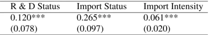
coefficients are positive and significant. Exporters have a higher probability of investing in R & D (the difference between exporters and non exporters is0.12), are more likely to import intermediate inputs from abroad (the difference between exporters and non exporters is0.27) and spend a higher proportion of their expenditure on intermediate inputs on imports (the average difference between exporters and non exporters is6.10percentage points.)

Table 2.1: Imports and R & D by Export Status

R & D Status Import Status Import Intensity

0.120*** 0.265*** 0.061***

(0.078) (0.097) (0.020)

Notes: Number of Observations is 45,835. Each column is a separate regression of the dependent variable on export status. Regressions control for firm size, Industry and Year effects. *** p<0.01, ** p<0.05, * p<0.1.

2.3 Empirical Production Function

In this section, I discuss the measure of total productivity used. Physical quantities and varieties of material inputs (both domestic and foreign) are not observed in the data. I move from the production technology as given by (2.1) and (2.2) to a specification which uses expenditure on intermediate inputs (domestic and foreign) as described in subsection 2.4.1. I also discuss how I retrieve estimates that reflect physical productivity by using firm level price deflators to measure output from firm revenues in subsection 2.4.2. This is in contrast to the literature which uses industry price deflators to measure output from firm revenues. The use of industry price deflators to measure output has some inherent problems which are addressed if information on firm prices is used instead.

2.3.1 The Production Function and Imports

on domestic intermediate inputs (Mdit =PdtXdit) . (See appendix A.2)

Pxit=Pdt

Mit Mdit

ρ−_ρ1

(2.21)

Since data on physical quantities of each of the input varieties used by the firm are not observed, I substitute forXitwith _PxitMit in the expression for the production technology of the firm. From (2.1)

and (2.30), the production function can thus be written as

Qit =eωitKitαkL αl itE αe it Mit Pdt αx Mit Mdit αχ (2.22)

whereαχ =αx

1−ρ

ρ

.

Usually, when production functions are estimated (including in the exports and productivity literature), the role of imported inputs is ignored. The last term in (2.31) is not included and the general form of the production function estimated is

Qit=eωitKitαkL αl itE αe it Mit Pdt αx (2.23)

Expenditure on inputs is deflated by a common input price deflator (usually a wholesale price index or an industry producer price index or a material inputs deflator). The term_MMit

dit

αχ gets subsumed in the estimate of productivityeωit_{. If all firms purchased all their inputs domestically,}

Mit Mdit

αχ

would disappear and (2.31) would reduce to (2.32).

However, for some firms, a portion of the expenditure on intermediate inputs is on inputs sourced from abroad. From (2.14) and (2.30),

Mit Mdit

= 1 +

"

pf_t(nit) θ−1

θ Pdt

#_ρ−ρ₁

(2.24)

Mit

Mdit is increasing innit and

Mit Mdit

αχ

the firm to produce a higher output.

Thus, we can think of firms with largernit(i.e., firms importing more foreign varieties) andωit

having a lower marginal cost of production as seen in section 2.2. Analogously, firms with higher import intensity (_MditMit) and higherωitare able to produce a higher level of output for a given level

of inputs.

The natural log of the production function (2.31) of firmican be written as

qit =αllit+αkkit+αeeit+αxmit+αχχit+ωit+it (2.25)

The lower case letters q, l, k, e, m, χ refer to the natural log of quantity, labor, capital, energy, expenditure on intermediate inputs and import intensity (_MM

d) of intermediate inputs respectively.

The measure of total productivity of interest is αχχit+ωit, the first component of which is

attributable to imports of intermediate inputs by the firm and the second to firm R & D. Firms can improve total productivity and lower marginal costs of production by importing foreign interme-diate inputs and engaging in R &D. The second component of the firm’s total productivityωit, is

known to the firm when it makes its decisions on inputs but is not observed in the data. Lastly,it

represents measurement error and idiosyncratic shocks to production. 2.3.2 Measuring Output based on Revenues and Prices

Since firm revenueRit = Pit∗Qit, firm output can be measured from firm revenues and firm

prices. If qit, pit and rit are the natural logarithm of firm output, firm prices and firm revenue

respectively,

qit =rit−pit (2.26)

Data on firm prices are often not available. Papers that estimate firm-level productivity (includ-ing the export-productivity literature) typically measure firm output by deflat(includ-ing firm revenues by an industry price deflator (pIt)which is common to all firms within an industryI. So they measure

the natural log of firm output as

e

Using (2.35) and (2.36), if we substitute forq_eit = qit−(pit−pIt)into (2.34), the production

function becomes

e

qit =αllit+αkkit+αeeit+αxmit+αχχit+ωeit+it (2.28)

where,

e

ωit = (pit−pIt) +ωit (2.29)

If firms operated in perfectly competitive markets where each firm was a price taker and charged the industry price (i.e, pit = pIt), (2.34) and (2.37) would be equivalent to each other.

However, when we deviate from the assumption of perfect competition (i.e,pit 6=pIt), two

prob-lems arise.

The first is the omitted price bias. In the absence of firm prices, if industry prices are used to measure output asq_eitinstead ofqit, the estimates of the coefficients of the production function will

be biased. As long as E[(pit −pIt)zit] 6= 0, where zit refers to the vector of inputs, the use of industry level price deflators to deflate revenues to proxy for output will yield incorrect estimates of the coefficients of the production function. (See Klette and Griliches (1996) for a detailed exposition of the omitted price bias).14

The second problem is specific to the export-productivity question when we try to estimate within firm changes to total productivity from export entry. If firms face downward sloping demand curves and pass on some of the benefits of gains in productivity to consumers by lowering prices,

pit falls as ωit rises. In this case, using estimates of productivity from (2.37) will underestimate

gains to firms’ post export market entry.15

14_{Everything else being equal, firms charging higher prices would have lower market shares. They would sell}

fewer units of output and employ fewer inputs i.e., price and inputs would be negatively correlated. However, more productive firms also need fewer inputs to produce the same output. So the relationship may not be so clear cut.

15_{Theoretical models of trade such as Melitz (2003b) model firms as operating in monopolistically competitive}

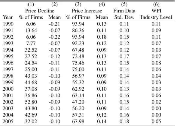
There is a wide variation in price changes across firms in a given industry in any year. I discuss concerns with using industry level price deflators to deflate firm revenues and use that to proxy for quantities by using the example of the transport equipment industry. Table 2.2 shows the yearly price change (over the previous year) for the transport equipment industry. The last column (6) gives the yearly price change as given by the Output Deflator of the transport equipment industry at the aggregate industry level as calculated by the Central Statistical Organization, Government of India. The average growth rates from the industry level indices are positive for every year in the period. Column (5) gives the standard deviation of firm price changes for each year as observed in the firm dataset.

Table 2.2: Price Changes in Transport Equipment Industry

(1) (2) (3) (4) (5) (6)

Price Decline Price Increase Firm Data WPI

Year % of Firms Mean % of Firms Mean Std. Dev. Industry Level

1990 6.06 -0.21 93.94 0.13 0.11 0.11

1991 13.64 -0.07 86.36 0.11 0.10 0.09

1992 6.06 -0.22 93.94 0.18 0.15 0.11

1993 7.77 -0.07 92.23 0.12 0.12 0.07

1994 32.52 -0.07 67.48 0.09 0.12 0.03

1995 27.52 -0.12 72.48 0.13 0.17 0.07

1996 24.54 -0.11 75.46 0.13 0.15 0.08

1997 25.00 -0.11 75.00 0.11 0.14 0.06

1998 43.03 -0.10 56.97 0.09 0.14 0.04

1999 44.68 -0.09 55.32 0.09 0.14 0.03

2000 37.08 -0.09 62.92 0.10 0.13 0.03

2001 36.86 -0.10 63.14 0.11 0.16 0.06

2002 52.80 -0.09 47.20 0.11 0.15 0.02

2003 43.80 -0.10 56.20 0.09 0.14 0.00

2004 42.69 -0.10 57.31 0.12 0.16 0.00

2005 32.02 -0.10 67.98 0.14 0.18 0.05

Notes: Column (6) shows price change for the for Transport Equipment Industry using the industry price deflator from the Government of India Price Statistics (WPI) from the 1993-94 price series. Columns (1)-(5) are constructed from firm level price data.

in prices over the previous year and the average increase in prices for the firms with positive growth. For example, in the year 2000, 37 % of firms saw on average a nine percent fall in their prices from 1999 while 63 % of the firms experienced a ten percent increase in prices on average. Price changes of firms varied widely as can be seen by the standard deviation. The use of the industry level deflator would assume that every firm experienced a three percent increase in prices over the previous year. Deflating revenues by the industry deflator would underestimate the quantity changes for firms with price changes less than three percent and overestimate the quantity changes for firms with growth in prices over three percent. This would imply that productivity change is underestimated for firms that experience a change in price of less than three percent and overestimated for firms that experience a change in price greater than three percent.

Information on prices allows me to estimate (2.34). I construct firm specific price deflators, which vary across firms within an industry, unlike industry level deflators that are common to all firms in an industry. I thus recover estimates of the production function coefficients andωitthat do

not suffer from the shortcomings discussed above.

2.4 Empirical Production Function

In this section, I discuss the measure of total productivity used. Physical quantities and varieties of material inputs (both domestic and foreign) are not observed in the data. I move from the production technology as given by (2.1) and (2.2) to a specification which uses expenditure on intermediate inputs (domestic and foreign) as described in subsection 2.4.1. I also discuss how I retrieve estimates that reflect physical productivity by using firm level price deflators to measure output from firm revenues in subsection 2.4.2. This is in contrast to the literature which uses industry price deflators to measure output from firm revenues. The use of industry price deflators to measure output has some inherent problems which are addressed if information on firm prices is used instead.

2.4.1 The Production Function and Imports

input bundle (Pdt), the total expenditure on intermediate inputs (Mit =PitXit) and the expenditure

on domestic intermediate inputs (Mdit =PdtXdit) . (See appendix A.2)

Pxit=Pdt

Mit Mdit

ρ−_ρ1

(2.30)

Since data on physical quantities of each of the input varieties used by the firm are not observed, I substitute forXitwith _PxitMit in the expression for the production technology of the firm. From (2.1) and (2.30), the production function can thus be written as

Qit =eωitKitαkL αl itE αe it Mit Pdt αx Mit Mdit αχ (2.31)

whereαχ =αx

1−ρ

ρ

.

Usually, when production functions are estimated (including in the exports and productivity literature), the role of imported inputs is ignored. The last term in (2.31) is not included and the general form of the production function estimated is

Qit=eωitKitαkL αl itE αe it Mit Pdt αx (2.32)

Expenditure on inputs is deflated by a common input price deflator (usually a wholesale price index or an industry producer price index or a material inputs deflator). The term_MMit

dit

αχ gets subsumed in the estimate of productivityeωit. If all firms purchased all their inputs domestically,

Mit Mdit

αχ

would disappear and (2.31) would reduce to (2.32).

However, for some firms, a portion of the expenditure on intermediate inputs is on inputs sourced from abroad. From (2.14) and (2.30),

Mit Mdit

= 1 +

"

pf_t(nit) θ−1

θ Pdt

#_ρ−ρ₁

(2.33)

Mit

Mdit is increasing innit and

Mit Mdit

αχ

expenditure on intermediate inputs, a higher import intensity represented by a larger _MditMit allows the firm to produce a higher output.

Thus, we can think of firms with largernit(i.e., firms importing more foreign varieties) andωit

having a lower marginal cost of production as seen in section 2.2. Analogously, firms with higher import intensity (_MditMit) and higherωitare able to produce a higher level of output for a given level

of inputs.

The natural log of the production function (2.31) of firmican be written as

qit =αllit+αkkit+αeeit+αxmit+αχχit+ωit+it (2.34)

The lower case letters q, l, k, e, m, χ refer to the natural log of quantity, labor, capital, energy, expenditure on intermediate inputs and import intensity (_MdM ) of intermediate inputs respectively.

The measure of total productivity of interest is αχχit+ωit, the first component of which is

attributable to imports of intermediate inputs by the firm and the second to firm R & D. Firms can improve total productivity and lower marginal costs of production by importing foreign interme-diate inputs and engaging in R & D. The second component of the firm’s total productivityωit, is

known to the firm when it makes its decisions on inputs but is not observed in the data. Lastly,it

represents measurement error and idiosyncratic shocks to production. 2.4.2 Measuring Output based on Revenues and Prices

Since firm revenueRit = Pit∗Qit, firm output can be measured from firm revenues and firm

prices. If qit, pit and rit are the natural logarithm of firm output, firm prices and firm revenue respectively,

qit =rit−pit (2.35)

Data on firm prices are often not available. Papers that estimate firm-level productivity (includ-ing the export-productivity literature) typically measure firm output by deflat(includ-ing firm revenues by an industry price deflator (pIt)which is common to all firms within an industryI. So they measure

the natural log of firm output as

e

Using (2.35) and (2.36), if we substitute forq_eit = qit−(pit−pIt)into (2.34), the production

function becomes

e

qit =αllit+αkkit+αeeit+αxmit+αχχit+ωeit+it (2.37)

where,

e

ωit = (pit−pIt) +ωit (2.38)

If firms operated in perfectly competitive markets where each firm was a price taker and charged the industry price (i.e, pit = pIt), (2.34) and (2.37) would be equivalent to each other.

However, when we deviate from the assumption of perfect competition (i.e,pit 6=pIt), two

prob-lems arise.

The first is the omitted price bias. In the absence of firm prices, if industry prices are used to measure output asq_eitinstead ofqit, the estimates of the coefficients of the production function will

be biased. As long as E[(pit −pIt)zit] 6= 0, where zit refers to the vector of inputs, the use of industry level price deflators to deflate revenues to proxy for output will yield incorrect estimates of the coefficients of the production function. (See Klette and Griliches (1996) for a detailed exposition of the omitted price bias).16

The second problem is specific to the export-productivity question when we try to estimate within firm changes to total productivity from export entry. If firms face downward sloping demand curves and pass on some of the benefits of gains in productivity to consumers by lowering prices,

pit falls as ωit rises. In this case, using estimates of productivity from (2.37) will underestimate

gains to firms’ post export market entry.17

16_{Everything else being equal, firms charging higher prices would have lower market shares. They would sell}

fewer units of output and employ fewer inputs i.e., price and inputs would be negatively correlated. However, more productive firms also need fewer inputs to produce the same output. So the relationship may not be so clear cut.

17_{Theoretical models of trade such as Melitz (2003b) model firms as operating in monopolistically competitive}

There is a wide variation in price changes across firms in a given industry in any year. I discuss concerns with using industry level price deflators to deflate firm revenues and use that to proxy for quantities by using the example of the transport equipment industry. Table 2.2 shows the yearly price change (over the previous year) for the transport equipment industry. The last column (6) gives the yearly price change as given by the Output Deflator of the transport equipment industry at the aggregate industry level as calculated by the Central Statistical Organization, Government of India. The average growth rates from the industry level indices are positive for every year in the period. Column (5) gives the standard deviation of firm price changes for each year as observed in the firm dataset.

Columns (1) and (2) report the percentage of firms that experienced decline in prices over the previous year and the mean reduction in prices over the previous year for firms with negative growth, while columns (3) and (4) give the percentage of firms that experienced positive growth in prices over the previous year and the average increase in prices for the firms with positive growth. For example, in the year 2000, 37 % of firms saw on average a nine percent fall in their prices from 1999 while 63 % of the firms experienced a ten percent increase in prices on average. Price changes of firms varied widely as can be seen by the standard deviation. The use of the industry level deflator would assume that every firm experienced a three percent increase in prices over the previous year. Deflating revenues by the industry deflator would underestimate the quantity changes for firms with price changes less than three percent and overestimate the quantity changes for firms with growth in prices over three percent. This would imply that productivity change is underestimated for firms that experience a change in price of less than three percent and overestimated for firms that experience a change in price greater than three percent.

Information on prices allows me to estimate (2.34). I construct firm specific price deflators, which vary across firms within an industry, unlike industry level deflators that are common to all firms in an industry. I thus recover estimates of the production function coefficients andωitthat do

2.5 Estimation Strategy

The empirical strategy involves two steps. First, I recover the parameters of the the production function and calculate estimates of total productivity (αχχit_c + ωit)_c . Next, I use difference-in-differences propensity score matching to examine the impact of starting to export on efficiency. 2.5.1 Recovering the Production Function Parameters

I estimate the parameters of (2.34) using proxy estimators for each industry separately. These methods use a control function in a firm specific decision to proxy for productivity and control for the simultaneity bias that arises because input demand and unobserved productivity are correlated. I follow Ackerberg et al. (2015) who extends Olley and Pakes (1996) and Levinsohn and Petrin (2003).18

Under the time to build assumption for capital, capital used in production in periodtis known in periodt−1. Given the restrictive labor laws in India on hiring, firing and closing down plants, there are adjustment costs to labor.19 I assume like Ackerberg et al. (2015), that labor is not completely mobile and is chosen att−bwhere0 < b < 1. Firms make decisions on importing intermediate inputs. There are fixed costs to imports which involve searching for suppliers, navigating customs procedures and getting delivery of inputs across borders. Under this setup, material inputs are not fully adjustable. I assume material inputs are chosen att−cwhere0< c <1. Energy inputs are fully flexible and are chosen at periodtafter capital, labor, material inputs (domestic and imported) and productivity is observed.20

The demand function for energy inputs is given by eit = h(kit, lit, mit, χit, ωit). Under the

18_{Ackerberg et al. (2015) argue that the labor parameter cannot be consistently identified in the Olley and Pakes}

(1996) and Levinsohn and Petrin (2003) method. They use the Value added production function because of concerns that the variable inputs would be perfectly correlated and thus collinear. While I use the gross output production function, I report the correlation matrix of all the input variables used in the production function in Table A.1 in appendix A.3. While the inputs are positively correlated as is expected, they are not perfectly correlated (with all correlations below .75).

19_{See Hasan, Mitra, and Ramaswamy (2007) for a discussion on labor market regulations and rigidities in India.}

20_{The exact ordering of the timing assumptions of when labor and material inputs are chosen does not impact the}

monotonicity assumption (the demand for the variable input h(kit, lit, mit, χit, ωit) is strictly

in-creasing inωit), the energy demand function can be inverted to proxy for unobserved productivity.

ωit =h−1(kit, lit, mit, χit, eit)is the inverse demand function for energy.

Under the Ackerberg et al. (2015) method, no coefficient of the production function is estimated in the first stage. The first stage is used to get a consistent estimate of expected output (φb_it(.)).

qit =φit(lit, kit, mit, χit, eit) +it (2.39)

where

φit=αllit+αkkit+αxmit+αχχit+αeeit+h−1(kit, lit, mit, χit, eit) (2.40)

In addition to the firm variables inh−1_{(.), I also include year dummies to account for macro trends} that could impact input demand.21_{. Once}

b

φit(.)is estimated for any candidate candidate values of

the coefficients, productivity can be written as

ωit(α) =φb_it−(α₀+α_ll_it+α_kk_it+α_xm_it+α_χχ_it+α_ee_it) (2.41)

For the candidate values of the coefficients, the productivity series can be used to estimate the productivity evolution as given by

ωit =γ1ωit−1+γ2dkit−1+γ3ωit−1∗dkit−1+ζit (2.42)

From (2.41) and (2.42),ζitcan be recovered for the candidate values of the coefficients. ωitis

decomposed into two parts. The first part constitutes the conditional expectation of productivity based on the information set known in period t−1. The second, ζit, is the deviation from the expectation. ζit is mean independent of the information known in t − 1 and is not correlated

with the past decisions of the firm. This provides the basis for the instruments for identifying the

21_{I use a fifth degree polynomial in capital, labor, material inputs, labor and energy to get an estimate of} b

coefficients through GMM using the moment conditions.

E(ζit(α, γ)Zit) = 0 (2.43)

The instrument set includes current capital kit (since it is chosen in t − 1) and lagged values

of the other variables (lit−1, mit−1, χit−1,eit−1, ditk−1, φb_it−1(.)andφb_it−1(.)∗dkit−1) to identify the production function parameters and the parameters of the productivity evolution process since they are all uncorrelated withζit.

2.5.2 Gains from Exporting

The overall productivity is α_cχχit+ωcit, which is constituted of two parts. The first is produc-tivity due to imports of intermediate inputs and the second is producproduc-tivity due to investment in R & D. To examine the impact of entry into export markets on firm productivity, I follow the micro-econometrics literature on program evaluation and estimate the average effect of treatment on the treated (ATT).22

In the context of this paper, treatment (W) is the entry into export markets and the outcome of interest (Yis) is productivity of firm i in period s. I define an export entrant as a firm that enters

into the export market for the first time and is an exporter for a minimum of two years. Also, the firms should have an observed history of at least two years in the data prior to export entry.

Since I do not observe the counter-factual of the outcome of interest had the treated firm not entered into the export market, I estimate propensity scores as proposed by Rosenbaum and Rubin (1983) to find a control group as close as possible to the treated group. W takes the value 1 if the firm begins to export and 0otherwise. To get a value for the counter-factual outcome if the exporting firm had not entered the export market, the control group is from the group of never exporters. The propensity score or the probability of entry into export markets is

P(Wit = 1) = Φ f(ωit−1, kit−1, lit−1, dkit−1, χit−1)

(2.44)

where P(Wit = 1) is the probability of the firm starting to export at period t, Φ is the

cumu-lative normal distribution and f(.) is a polynomial of the variables. I also include a full set of year and industry effects in the equation. The panel dataset allows me to implement a Difference-in-Differences (DID) matching estimator as suggested by Heckman et al. (1997). Blundell and Costa Dias (2000) note that combining matching with DID allows for the possibility of unob-servables affecting participation if they can be represented by separable firm specific and /or time specific components.

Matching treated and control groups on propensity scores requires two assumptions. The com-mon support assumption requires the possibility of a non treated counterpart for each treated firm. It is given byP(W = 1)|P <1, whereP is the propensity score.

The conditional mean assumption requires that the expected change in outcome of the treated firm had it not been treated should be the same as the expected change in outcome of the control firm i.e.,E(Y0

t0 −Y_t0₋₁|P, W = 1) =E(Y_t00 −Y_t0₋₁|P, W = 0). Here,t−1denotes the time period just prior to export entry,t0 =t+iwherei= 1,2,3,4...denote time periods after export entry and

(Y_t00−Y_t0₋₁)denotes the change in the outcome of interest between the two periods in the untreated state.

The treatment on the treated is given by

δτ = 1 N

X

i∈T

(Y_it10 −Y_it1₋₁)− X

j∈C

wij(Yjtc0 −Y_jtc₋₁) !

(2.45)

Here N refers to the number of firms that start to export, T refers to the treated group i.e., the export starters andCrefers to the control group of never exporters. Each firmi∈T is matched to firms in the control group andwij is the weight on each firmj in the control group as a match for

firmi. 23 Y1

it0 −Y_it1₋₁ is the change in the outcome variable for the export entrant betweent0 and

t−1andYc

jt0 −Y_jtc₋₁ is the change in the outcome variable for the control firms betweent0 and

t−1.

23_{For example, a nearest neighbor matching with one neighbor would mean that for firm i ∈ T, the firm most}

The outcomes of interest are(α_cχχit+ωcit)as well as the individual componentsαcχχitandωcit, to examine whether overall productivity improves on export entry as well as the relative importance of the two different channels.

2.6 Data

The firm level variables are from the Prowess dataset provided by the Center for Monitoring of the Indian Economy (CMIE). This is a panel dataset of Indian firms in the organized sector. It includes both listed and unlisted firms. The dataset has been used in several papers including Goldberg et al. (2010) and Topalova and Khandelwal (2011).

I use data on firm observations from1989to2005. For these years, there is information on all the firm variables used in the production function estimation as well as quantities and sales values of products of firms. There are data on5,850manufacturing firms with45,835firm year observa-tions. The firms belong to thirteen major industry groups.24 Industries are classified according to the National Industrial Classification (NIC2008). There is a one to one correspondence between the NIC and ISIC (The United Nations International Standard Industrial Classification).

The dataset is appropriate for this study because it tracks firm performance over time for a variety of variables. In addition to the usual variables on revenue and inputs, which are relevant for productivity estimation, it also contains data on variables relating to firm activity in international markets (exports and imports) as well as on investment in knowledge (R & D spending). It also has product level data on all products produced by the firm which allows for the construction of firm specific price deflators.

All input variables have been deflated to1989−90levels using deflators from the 1993−94

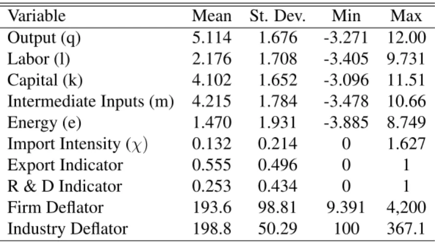
price series. Energy, Wages and Capital Stock were deflated by the power and fuel, wholesale price index and machinery deflators respectively. I created input price deflators for each industry by passing output deflators through the input-output matrix for each industry. Summary statistics for the variables used in the production function are reported in Table 3.3.

The measure of quantity I use is the firm sales revenue deflated by the firm specific price

24_{I exclude minor industries such as printing, coke and petroleum products etc., where the number of firm year}

deflator. The import intensity term is the total expenditure on intermediate inputs divided by the expenditure on domestic inputs. All firm output and input variables (quantity, labor, capital, energy, material inputs and import intensity) are expressed as natural logarithms while the export and R & D indicator are discrete variables. There are544 export entrants where an export entrant is as defined in subsection 2.5.2.

The dataset contains information on the number of units sold as well as total sales value of the product for each product of the firm. This gives us unit values of the product. There are data on about150,000product year observations. 1,658firms are single product firms throughout the period while the remaining firms sell two or more products at at least some point in the pe-riod. Products are assigned a product code based on the product classification developed by CMIE Prowess. Each product code is matched to a five digit industry.

I follow Eslava, Haltiwanger, Kugler, and Kugler (2004), Eslava, Haltiwanger, Kugler, and Kugler (2010) and Ornaghi (2008) to construct firm-specific price deflators as Tornqvist indices of the weighted average growth of prices of all products produced by the firm. (See appendix A.2.1). I report the summary statistics for price deflators constructed from the firm data as well as industry deflators from the price series data from the Government of India Statistics Division in the last two rows of Table 3.3.

Table 2.3: Summary Statistics

Variable Mean St. Dev. Min Max

Output (q) 5.114 1.676 -3.271 12.00

Labor (l) 2.176 1.708 -3.405 9.731

Capital (k) 4.102 1.652 -3.096 11.51

Intermediate Inputs (m) 4.215 1.784 -3.478 10.66

Energy (e) 1.470 1.931 -3.885 8.749

Import Intensity (χ) 0.132 0.214 0 1.627

Export Indicator 0.555 0.496 0 1

R & D Indicator 0.253 0.434 0 1

Firm Deflator 193.6 98.81 9.391 4,200

Industry Deflator 198.8 50.29 100 367.1

2.7 Results

I begin by estimating the parameters of the production function (2.34) and the endogenous productivity evolution process (2.42) as described in subsection 2.5.1. The estimates are presented in subsection 2.7.1. In subsection 2.7.2, I discuss the baseline results of the gains from starting to export on overall productivity. I also present the estimates from the two separate components - productivity growth from imports of intermediate inputs, and productivity growth from R & D. Finally, in subsection 2.7.3, I present results from robustness checks.

2.7.1 Production Function Parameters: Imports and R & D

Tables 2.4, 2.5 and 2.6 present the results for the parameters of the production function and productivity evolution process. All these three sets of parameters are estimated simultaneously for the output production function where output of the firm is constructed from deflating firm revenues with the firm specific price deflator.

Table 2.4 reports the estimation results for the production function parameters for thirteen ma-jor manufacturing industry groups. αl, αk, αx, αe represent the share of labor, capital, material

inputs and energy inputs respectively in the production function. The magnitude of these parame-ters are reasonable across industries for these different inputs.25

The table also presents the output from the Wald test for constant returns to scale. The null hypothesis of constant returns to scale is rejected in seven out of the thirteen industries at the 10 percent level (and in six of the thirteen at the 5 percent level). Marin and Voigtlander (2013) use marginal cost as their measure of efficiency to capture productivity improvements through export entry. Marginal costs may decline not just because of productivity improvements but also with changes in capital stock. They show in their paper that, under the assumption of constant returns to scale, changes in marginal costs would reflect changes in productivity.

25_{Once the coefficients are estimated, theωvalues are calculated. In appendix A.3, I graph the overall distribution}

When technology does not exhibit constant returns to scale, changes in marginal costs would also be capturing changes in capital stock. In the context of Indian manufacturing, where about half the industries do not exhibit constant returns to scale, the approach used in this paper, where productivity is directly measured, is more appropriate rather than the use of marginal cost as a measure to capture productivity changes.

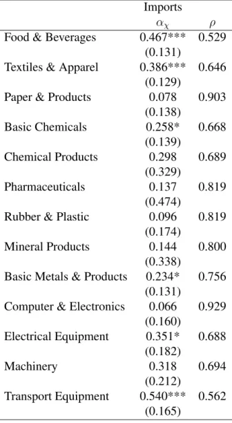
Table 2.5 presents the estimates of the imported inputs term in the production function. αχ is

the estimate on the import intensity term (χ) in the production function where χtakes a value 0

if the firm does not import from abroad (since in that case, Mit = Mdit and χ is the natural log

of _MditMit ). χis increasing in the expenditure share on imported intermediate inputs. The coefficient (αχ) is positive in all thirteen industries. Everything else held equal, firms that import a larger share

of their intermediate inputs from abroad are able to produce higher output with the given inputs. To illustrate, in the transport equipment industry, a10percent increase in the _MditMit ratio (which is approximately a9 percent decline in the expenditure share of domestic inputs in total inputs), while holding all inputs fixed (capital, labor, energy and total expenditure on intermediate inputs) will result in a5.4percent increase in total output.

The table also presents the implied values forρwhich are calculated from the estimates ofαx

andαχ for each of these industries since αχ = αx

1−ρ

ρ

. The elasticity of substitution between the domestic and imported input bundle is given by ₁₋1_ρ. The CES model restricts the value ofρto be between 0 and 1. The implied values forρfor all the thirteen industry groups falls within this range.

Table 2.6 presents the estimates of the endogenous productivity process. The coefficient γ1 measures the impact of previous period firm productivity on current productivity and is positive in all industries. The coefficientγ2 measures the average impact of the lagged discrete decision to invest in R & D on current productivity and is positive in all industries. Firms that undertake investment in R & D have on average,2to5percent higher productivity than firms that do not.

Table 2.5: Imports in the Production Function

Imports

αχ ρ

Food & Beverages 0.467*** 0.529 (0.131)

Textiles & Apparel 0.386*** 0.646 (0.129)

Paper & Products 0.078 0.903

(0.138)

Basic Chemicals 0.258* 0.668

(0.139)

Chemical Products 0.298 0.689

(0.329)

Pharmaceuticals 0.137 0.819

(0.474)

Rubber & Plastic 0.096 0.819

(0.174)

Mineral Products 0.144 0.800

(0.338)

Basic Metals & Products 0.234* 0.756 (0.131)

Computer & Electronics 0.066 0.929 (0.160)

Electrical Equipment 0.351* 0.688

(0.182)

Machinery 0.318 0.694

(0.212)

Transport Equipment 0.540*** 0.562 (0.165)

Table 2.6: Productivity Evolution: Past Productivity and Investment in R & D

ωt−1 dkt−1 ωt−1Xdkt−1

γ1 γ2 γ3

Food & Beverages 0.052 0.016* 0.697***

(0.047) (0.009) (0.087)

Textiles & Apparel 0.321** 0.025*** 0.500***

(0.144) (0.007) (0.161)

Paper & Products 0.422*** 0.046* 0.095

(0.095) (0.024) (0.309)

Basic Chemicals 0.762*** 0.000 -0.391***

(0.047) (0.028) (0.139)

Chemical Products 0.662*** 0.024** 0.354**

(0.096) (0.012) (0.165)

Pharmaceuticals 0.565*** 0.032*** 0.322**

(0.081) (0.009) (0.140)

Rubber & Plastic 0.778*** 0.024** 0.151*

(0.039) (0.011) (0.081)

Mineral Products 0.094 0.042*** 0.960***

(0.331) (0.008) (0.333)

Basic Metals & Products 0.694*** 0.024*** 0.273***

(0.042) (0.005) (0.051)

Computer & Electronics 0.224 0.011 0.432*

(0.164) (0.023) (0.238)

Electrical Equipment 0.001 0.035*** 0.845***

(0.001) (0.010) (0.087)

Machinery 0.317 0.033*** 0.994**

(0.241) (0.012) (0.415)

Transport Equipment 0.521*** 0.022*** 0.397*

(0.123) (0.005) (0.240)

industries, this term is positive. This implies that the productivity gains from investing in R & D is higher for more productive firms in almost all industries across the board. To illustrate, the difference in productivity growth is 1.9percentage points for a median productivity firm that engaged in R & D in the previous period compared to one that did not engage in R & D in the previous period. This difference is about18.6percentage points for a firm in the 90th percentile of productivity.26

2.7.2 Gains from Export Entry

I begin by graphically showing the productivity trajectory of an export entrant who has starting exporting in periodt= 0. Figure 2.1 depicts the productivity trajectory for the export entrant using measures of revenue productivity as well as physical productivity.27 I plot average productivity on the vertical axis while the horizontal axis depicts time. Here, revenue productivity is the produc-tivity measure retrieved when sales revenue are deflated by industry deflators and this is used to proxy for output in the production function. Physical productivity measures I have used are where sales revenues are deflated by firm specific deflators and used as a measure of firm output in the production function.

As can be seen in the graph, the export entrant’s revenue productivity is more or less stagnant over the six years following export entry. On the other hand, the average productivity (physical) of the export entrant increases and continues to rise from the time the firm begins to export. These different productivity trajectories highlight the need to retrieve measures of productivity that cap-ture physical productivity to estimate gains from export entry. I refer to the physical productivity measure as total productivity.

While Figure 2.1 shows that average total productivity rises for an export entrant, it does not indicate how differently productivity would have evolved had the firm not started exporting. In Fig-ure 2.2, I graph how the productivity trajectory of an export entrant compares with a non exporter

26_{Median productivity of a firm in the transport industry equals−.008while a 90th percentile firm has productivity}

which equals.414. The parameters of the productivity process in the transport industry areγ1 = 0.521,γ2 =.022 andγ3= 0.397

27_{These productivity trajectories are based on348export entrants for which data are available for the entire period}

Figure 2.1: Productivity Trajectory for Export Entrant (Revenue vs. Physical Productivity) Average Firm Specific Total Productivity