STATISTICAL LEARNING WITH MISSING DATA
Thomas Gordon Stewart
A dissertation submitted to the faculty at the University of North Carolina at Chapel Hill in partial fulfillment of the requirements for the degree of
Doctor of Philosophy in the Department of Biostatistics.
Chapel Hill 2015
c
2015
ABSTRACT
Thomas Gordon Stewart: Statistical Learning with Missing Data (Under the direction of Michael Wu and Donglin Zeng)
ACKNOWLEDGEMENTS
I could not have completed this dissertation without the patient and kind help of Michael Wu and Donglin Zeng. I am indebted to them for their mentoring, encour-agement, and support. To each, I offer sincere appreciation and gratitude. Thank you Michael and Donglin.
My time at UNC was enriched with many interesting projects with talented collaborators. Foremost of these projects is my work with Paul Stewart and HCV-TARGET. I consider my association with Paul and each member of the HCV-TARGET family as one of the great, unforeseen experiences of my graduate school career. Not only did HCV-TARGET support me financially, it gave me a chance to develop into a consulting statistician. Thank you to Paul Stewart, Monica Vainorius, Lucy Akushe-vich, Ken Bergquist, John Baron, and Michael Fried.
Veronica Stallings and Melissa Hobgood are the cheerful core of the Biostatistics Department. My time in the department has been improved by their laugh, encour-agement, and administrative finesse. Thank you Veronica and Melissa.
TABLE OF CONTENTS
LIST OF TABLES . . . xii
LIST OF FIGURES . . . xiv
CHAPTER 1: LITERATURE REVIEW . . . 1
1.1 Introduction . . . 1
1.2 Parametric and semi-parametric methods for missing data . . . . 2
1.2.1 Missing data mechanism . . . 2
1.2.2 Complete case analysis and imputation methods . . . 4
1.2.3 Parametric and semi-parametric methods . . . 5
1.3 Statistical learning methods for missing data . . . 9
1.3.1 Plug-in method . . . 10
1.3.2 Discriminant analysis . . . 13
1.3.3 Trees based methods . . . 15
1.3.4 k-nearest neighbor . . . . 18
1.4 Support Vector Machines . . . 19
1.5 Multi-class Support Vector Machines . . . 30
1.5.1 Composite-of-binary SVMs . . . 30
1.5.2 Simultaneously Trained SVMs . . . 32
1.6 Semi-supervised Learning and Support Vector Machines . . . 33
1.6.2 Maximum Margin Clustering . . . 35
1.7 Dissertation topics . . . 37
CHAPTER 2: AUGMENTED AND WEIGHTED SUPPORT VECTOR MACHINES FOR MISSING COVARIATES . . . 39
2.1 Introduction . . . 39
2.2 Method . . . 41
2.2.1 Properties of the AWSVM . . . 44
2.3 Simulation Study . . . 45
2.3.1 Results . . . 45
2.4 Application to HCV-TARGET Data . . . 50
2.5 Conclusion . . . 53
CHAPTER 3: DOUBLY ROBUST SUPPORT VECTOR MACHINES FOR MISSING COVARIATES . . . 56
3.1 Introduction . . . 56
3.2 Methods . . . 59
3.2.1 Support Vector Machine Classifiers . . . 59
3.2.2 Doubly Robust Support Vector Machine . . . 60
3.2.3 Computation of the DRSVM . . . 62
3.2.4 Doubly Weighted SVM Classifier . . . 64
3.3 Simulation Study . . . 65
3.3.1 Simulation Scenarios . . . 65
3.3.2 Simulation results . . . 68
3.4 Application to HCV-TARGET Study . . . 71
3.6 Acknowledgments . . . 76
CHAPTER 4: SUPPORT VECTOR MACHINES FOR PARTIALLY OBSERVED OUTCOMES . . . 77
4.1 Introduction . . . 77
4.1.1 Two-class and Multi-class Support Vector Machines . . . . 78
4.1.2 Missing class labels . . . 80
4.2 Methods . . . 84
4.2.1 The Reinforced Multi-class Support Vector Machine . . . . 84
4.2.2 Proposed Method for Missing Class Labels . . . 86
4.2.3 Partially Observed Outcomes . . . 89
4.2.4 Properties . . . 89
4.2.5 Computation . . . 90
4.2.6 Improvements for two-class and multi-class settings . . . . 91
4.3 Simulation Study . . . 92
4.3.1 Classification with Partially-Observed Outcomes . . . 92
4.3.2 Results of Partially-Observed Outcomes Simulation . . . . 93
4.3.3 Semi-supervised classification . . . 94
4.3.4 Results . . . 95
4.4 Application to Real Datasets . . . 97
4.4.1 Application to HCV-TARGET data . . . 97
4.5 Conclusion . . . 99
4.6 Acknowledgments . . . 99
5.1 Re-weighting Instead of Tuning . . . 100
5.1.1 SVMs and NMAR Data . . . 102
5.1.2 Causal Inference and Statistical Learning . . . 103
APPENDIX A: AWSVM PROPOSITIONS AND ADDITIONAL RESULTS . . . 104
A.1 Proposition 1 . . . 104
A.2 Proposition 2 . . . 108
APPENDIX B: RESULTS AND PROPOSITIONS FOR WEIGHTED SUPPORT VECTOR MACHINES . . . 110
B.1 Proposition 1 . . . 110
B.2 Proposition 2 . . . 111
B.3 Proposition 3 . . . 114
B.4 Simulation Results for Doubly Robust SVM . . . 117
APPENDIX C: PROPOSITIONS AND RESULTS FOR PARTIALLY OBSERVED OUTCOME SUPPORT VECTOR MACHINES . . . 122
C.1 Proposition 1 . . . 122
C.2 Proposition 2 . . . 124
C.3 Constructing a weighted multi-class SVM classifier . . . 126
C.4 Constructing a multi-class SVM classifier with fewer basis functions . . . 131
C.5 Simulation Study Results for Partially-observed Outcomes . . . . 136
C.6 Simulation Study Results for Semi-supervised Learning . . . 147
LIST OF TABLES
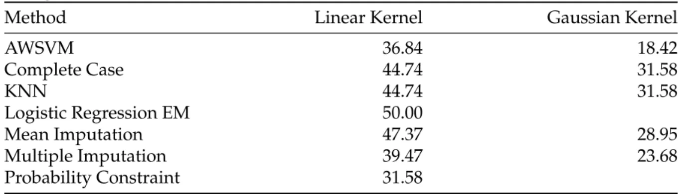
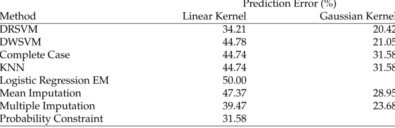
2.1 AWSVM Algorithm . . . 43 2.2 Prediction Error of Competing Classification Methods
Applied to HCV-TARGET Data . . . 53
3.1 Subset of Simulation Results (Full results are in the Appendix) . . . 72 3.2 Prediction Error of Competing Classification Methods
Applied to HCV-TARGET Data . . . 74
4.1 Selection of Simulation Results, Partially Observed Outcomes . . . 94 4.2 Summary of Semi-supervised Learning Simulation
Restricted to Low and Medium Classification Risk Settings . . . 96 4.3 Prediction Error of Semi-supervised SVM Methods
Applied to HCV-TARGET Varices Data . . . 98
B.1 Simulation Results (2 Covariates, Missingness depends
on Y and X) . . . 118 B.2 Simulation Results (2 Covariates, Missingness depends on X) . . . 119 B.3 Simulation Results (10 Covariates, Missingness
depends on Y and X) . . . 120 B.4 Simulation Results (10 Covariates, Missingness depends on X) . . . 121
C.1 Simulation results of methods for partially-observed
outcomes,N=40 for smallest class . . . 137 C.2 Simulation results of methods for partially-observed
outcomes,N=100 for smallest class . . . 138 C.3 Simulation results of semi-supervised methods by
C.5 Simulation results of semi-supervised methods by
LIST OF FIGURES
1.1 Example of classification tree . . . 16 1.2 SVM Demonstration, toy data . . . 20 1.3 Examples of Two SVM Classifiers . . . 26
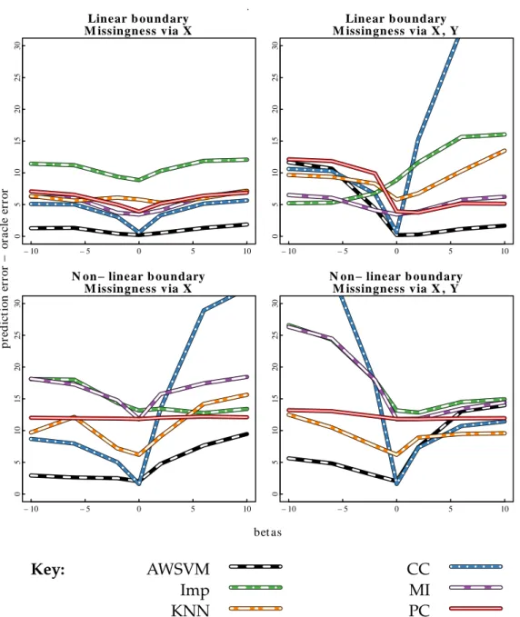
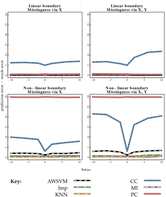
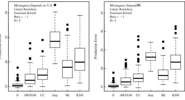
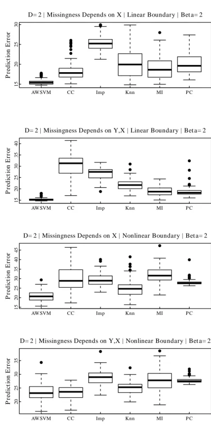
2.1 Comparison of AWSVM to competitors, simulation
results ford=2 predictors. . . 48 2.2 Comparison of AWSVM to competitors, simulation
results ford=20 predictors. . . 49 2.3 Prediction error when the boundary is linear and the
decision rule is constructed with a Gaussian kernel . . . 50 2.4 Comparison of Prediction Error Variability of
Commonly Used Missing Data Methods . . . 51 2.5 Plots of AWSVM decision rule constructed with
HCV-TARGET data. . . 54
4.1 Schematic of EM algorithm for RMSVM with missing class labels . . . . 88
5.1 Simulation Results Comparing the Prediction Accuracy of Re-weighted Tuning and Cross Validation Tuning of
the Cost Parameter . . . 102
C.1 Simulation results of methods for partially-observed
outcomes, linear SVMs,N=40 per class . . . 139 C.2 Simulation results of methods for partially-observed
outcomes, linear SVMs,N=100 per class . . . 140 C.3 Simulation results of methods for partially-observed
outcomes, nonlinear SVMs,N=40 per class . . . 141 C.4 Simulation results of methods for partially-observed
C.5 Simulation results of methods for partially-observed
outcomes, side-by-side comparison, linear SVMs,N =40 per class . . . 143 C.6 Simulation results of methods for partially-observed
outcomes: side-by-side comparison, nonlinear SVMs,
N=40 per class . . . 144 C.7 Simulation results of methods for partially-observed
outcomes, side-by-side comparison, linear SVMs,N =100 per class . . 145 C.8 Simulation results of methods for partially-observed
outcomes: side-by-side comparison, nonlinear SVMs,
CHAPTER 1: LITERATURE REVIEW
1.1 Introduction
Missing data are ubiquitous. Despite continuing advances in data collection, missing data are likely to remain a permanent feature of statistical analysis. While many missing data methods exist for multivariate normal models [47], general likeli-hood models [89, 28], survey sampling models [90], and weighted estimating equation models [86], all the developments are either parametric or semi-parametric methods, so they are sensitive to model miss-specification and may not be applicable in high dimensional settings.
special attention to support vector machines (SVM) because it is the focus of methods for missing data proposed in the following chapters. The support vector machine is a statistical learning method introduced in Boser et al. [15], Cortes and Vapnik [25] and Vapnik [106]. The method has been successfully employed in both classification and regression tasks, and it is particularly useful in computer vision applications [77, 23]. It is a basis expansion method which provides the user with considerable modeling flexibility.
The literature review is organized into four sections. The first is a review of Rubin [89] and many of the parametric or semi-parametric methods that followed. We introduce likelihood with EM, imputation, weighted estimating equations, and Bayesian methods for missing data. The second section is an overview of binary supervised classification methods and their associated methods for missing data. The third section particularly focuses on SVM and describes its methods for missing data. Lastly, we describe a research plan which provides three principled missing data methods.
1.2 Parametric and semi-parametric methods for missing data
1.2.1 Missing data mechanism
Consider a training data set of n observations with outcome yi and covariate
vector xi of dimension d for each patient. Depending on the scenario, outcomes or
covariates may be missing. To indicate which variables are missing, letzi =(yi,xi) and
define vectorrito indicate if the corresponding data element inziis observed or not,
ri =(ri0,ri1,ri2, . . . ,rid) rij =
10 ififzzijij is observedis missing.
three types. The simplest type of missing data mechanism is missing completely at random (MCAR). MCAR describes situations when the missing data mechanism is independent of the data. In terms of the missing data indicator, MCAR mechanisms are characterized as
P(ri|zmi , zoi)=P(ri).
In other words, the mechanisms which lead to missing data are unrelated to either outcome or predictors. The second type of missing data mechanism is missing at random (MAR). It occurs if, conditional on the observed data zo, the missing data
mechanism is independent of the missing datazm. That is,
P(ri|zmi , zio)=P(ri|zoi).
Lastly, not missing at random (NMAR) occurs if the missing data model is a function of the unobserved missing value. The missing value is unobserved for reasons related to the value. In the notation of missing data models, NMAR is
P(ri|zmi , zoi)=P(ri|zmi , zoi),
or any distribution which depends onzm
i . The three types of missing data represent a
hierarchy of modeling assumptions. MCAR is the strongest assumption while NMAR is the weakest.
mechanism under these two assumptions. In contrast, if the missing data are NMAR, likelihood and Bayesian methods must incorporate the unverifiable assumptions of a missing indicator model. In the sections that follow, we will discuss methods and identify them as being applicable to MAR data or MCAR data.
1.2.2 Complete case analysis and imputation methods
Perhaps the earliest and easiest method for handling missing data is to omit ob-servations with missing values, a method known as complete case analysis. Complete case analysis is valid in MCAR situations, but is not valid with MAR data.
Imputation is a two-stage method and is popular because it works with a wide variety of models and estimation techniques. One of its earliest forms was developed and used extensively with the Current Population Survey by the US Census Bureau, despite its poorly developed theory [4]. In the context of large scale surveys, Rubin [90] introduced multiple imputation and provided conditions for the method’s appli-cation to unbiased estimation, also see Schafer [93], Harel and Zhou [46] and Rubin [91]. There are two general imputation types: single and multiple. The single impu-tation procedure is to replace missing values with values drawn from an impuimpu-tation model. The filled-in or complete data set is analyzed with the desired method. As noted in Rubin [90], single imputation standard error estimates are generally too small because uncertainty from the imputations is not incorporated into the standard error calculations.
very similar estimates, the imputation error leads to a small increase in standard error. Conversely, disparate estimates lead to a larger standard error.
Depending on the analysis method and its attendant assumptions, the imputa-tion model can be chosen so that resulting estimates are unbiased in cases of MCAR or MAR data [90]. However, when missing values are drawn from a convenience distribution instead of the proper imputation distribution, the imputation model is improper. Estimates calculated from improper imputation can be reasonable, but there is no assurance that the estimates are unbiased.
1.2.3 Parametric and semi-parametric methods
Here we consider the methods for missing data in three broad families of param-eter estimation: likelihood estimation, estimating equations, and Bayesian estimation. The methods described here can be generalized to a wide variety of classification and regression methods. In each method, we consider estimation of some population parameterβ.
Likelihood estimation and EM
In the context of likelihood estimation of a regression model, say ofy=xtβ+ǫ, with MAR missingness in the covariates, Rubin [89] noted that estimation only requires maximization of the observed data likelihood. Thus, if P(y|x, β) is the likelihood and P(xm|xo,α) is the covariate distribution, then the observed data likelihood to be
maximized is
L(β,α)=
n
Y
i
Z
P(yi|xi,β)P(xmi |xoi,α)dxmi . (1.1)
are already available. One starts the algorithm by postulating values for parameters β(0)andα(0). Then, the iterations of the algorithm consist of two steps. In the first, one
replaces the unobserved complete data log-likelihood with its expectation conditional on the observed data, and postulated values of model parameters,
E{ℓ(β,α)|Xo,y,β(0),α(0)}=
n
X
i=1
E{log[P(yi|xi,β)]|xoi,yi,β}
+
n
X
i=1
E{log[P(xmi |xoi)]|xoi,yi,α}.
At the second step and with the expectation in hand, one maximizes the log likelihood as if the data were fully observed. The estimates ˆβ and ˆα update the previously postulated model parameters,β(1) =βˆ andα(1) =α. The expectation and maximizationˆ steps repeat, each time updating the postulated parameter values with the estimates. The repeated two steps give rise to the name EM: expectation and maximization. The EM iterations continue until the model parameters converge.
Louis [70] provided formulas to estimate variance and covariance via the ob-served information matrix. Wu [109] defined regularity conditions and provided convergence properties for the EM algorithm. Although EM is guaranteed to con-verge under mild conditions, the rate of concon-vergence can be slow. In light of the slow convergence, several researchers have proposed modifications to improve speed; these include Meng and van Dyk [73], Meng and van Dyk [72], Berlinet and Roland [13], and Liu and Rubin [67].
and Ibrahim [53] applies EM to cure rate models with random effects when there is non-ignorable missingness in the predictors. The successful application of the EM algorithm to parametric and semi-parametric models is substantial, and it highlights the method’s utility.
Weighted estimating equations
Likelihood estimation can be seen as a member of a broader family of estimation methods known as estimating equations. Introduced in Godambe [43] and Godambe and Thompson [44], an estimating equation for parameter β is a function ψ(y,x,β) which satisfies the expression
EP[ψ(y,x,β)]=0. (1.2)
Estimation ofβis based on the empirical expectation; the estimate ˆβis selected so that
n
X
i
ψ(yi,xi,β)ˆ =0.
The estimate is unbiased, and the method is free of any specific distributional assump-tions. Estimating equations are a framework often used in causal inference and robust estimation research. Robins et al. [86] and Bang and Robins [8] introduced weighted estimating equations as a missing data method. The method, known as the doubly robust estimator, builds on earlier ideas known as inverse probability weighting. We summarize both. Let ˙ri indicate if patientiis a complete case.
The inverse probability weighted (IPW) method starts with the selection prob-ability,pi =P( ˙ri =1|xoi,yi). The estimate ˆβis selected so that
n
X
i
˙ ri
pi
Only complete case observations contribute to the estimating equation, but value 1/pi
weights each observation so that the expectation of the estimating equation is the desired output. For example, if missingness is a function of gender and responses are less likely from males, the inverse selection probability up-weights males and down-weights females so that the resulting average reflects the entire population and not the complete case sample.
The doubly robust (DR) estimator builds on the IPW. The key improvement of the DR estimator over the IPW estimator is that incomplete cases contribute to the estimating equation. This is achieved with a surrogate function, φ(Y,Xo, θ), which
takes the place ofψfor incomplete cases. The DR estimating equation is
n
X
i
˙ ri
piψ(yi,
xi,β)−
˙ ri
pi −
1
!
φ(yi,xoi,β).
Bang and Robins [8] shows that the resulting estimator is consistent if either (a) the estimates ofpiare correct or (b) the surrogate functionφapproximates well the function
ψ. For optimal efficiency, the surrogate function is selected as
φ(yi,xoi,β)=E[ψ(yi,xi,β)|yi,xoi],
which in practice is often approximated with imputation techniques. See Carpenter et al. [18], Vansteelandt et al. [105], and Ibrahim et al. [57] for reviews of DR estimators. Note that likelihood based estimation can be framed within estimating equations. The score function S(β) = ∂ℓ∂β(β) can be an estimating equation ψ. Thus, the IPW and DR missing data methods can apply to likelihood estimation as well.
Bayesian estimation
data. Like likelihood methods, it begins with a likelihood function P(y|x,β), a data model P(xm|xo,α), and possibly a missing data model P(r|φ). One also assumes a
prior distribution P(β,α,φ) for the model parameters. Estimates of β are based on the observed data posterior distribution P(β|xo,y). Operationally, Bayesian analyses usually involve sequential sampling methods, like Gibbs, to draw from the complete data posterior distribution. Without missing data, the sampling sequence at each iteration draws from (a) P(β|α,xo,xm,y) then (b) P(α|β,xo,xm,y). With missing data,
the sequence also includes draws from (c)P(xm|α,β,xo,y). Inference about βis based
on summaries of the resulting sample.
1.3 Statistical learning methods for missing data
In this section, we discuss a general framework for supervised classification methods and properties of optimal classifiers. Additionally, we discuss several sta-tistical learning classifiers and their associated missing data methods. This summary covers binary classification, though the concepts can be generalized to classification into several groups.
To begin, we introduce notation specific to classification in the context of a patient population where the outcome is cure status. Those that are cured, label yi = +1; label all others yi = −1. Let y and x denote the outcome and covariates
of a generic patient not in the training set Tn. The classification task is to construct a classification rule f : Rd → {±1} which predicts cure status y from inputs x. To measure classification performance, consider the four possible outcomes of a classifier for a single patient:
y f(x) +1 -1
The relative importance of error A to error B depends on the specific application; when both errors are penalized equally, classification error is captured by the c-loss function Lc[yo, f(x)] = I[yo , f(x)] or equivalently I[yof(x) < 0]. The performance of
any classification rule is measured in terms of average classification error (or risk) which is defined as
RLc,P(f)=EP
n
Lc[yo, f(x)]
o
(1.3)
wherePdenotes the distributionP(y, x). Optimal classifiers minimizes this quantity. Such classifiers are known as Bayes classifiers, and the minimum classification risk is the Bayes risk, i.e.,
fbayes(x)=arg min
f RLc,P(f) and RLc,P(fbayes)
=min
f RLc,P(f).
If the distributionP(y, x) is known, then the Bayes classifier can be calculated directly as
fbayes(x)=sign
P(y= +1|x)− 1
2
. (1.4)
Many of the methods discussed in this section are plug-in estimates, in that the primary endeavor of several methods is to generate an estimate of P(y = +1|x). In fact, the methods that follow can be classified into four groups. The first group assumes a distribution, usually some form of the Bernoulli distributionP(y|θ(β,x)) whereθ(β,x) is the odds parameter and a function ofx and β. The second endeavors to estimate the conditional distribution without parametric assumptions. The third group is the distribution free k-nearest neighbors. And, the last group approaches the problem with empirical risk minimization.
1.3.1 Plug-in method
a standard likelihood and Bayesian model. In the context of classification performance and finding a Bayes classifier, the logistic regression model starts with the assumption thaty|xis a Bernoulli random variable with odds parameterθ(β,x). Thus, onceθ(β,x) is estimated, the modelP[y|θ(x)] can be plugged into equation (1.4) as an estimate of the Bayes rule. If the distribution and modeling assumptions are correct, the resulting classifier is asymptotically a Bayes classifier.
The simplest model of log odds is the linear model. It is:
log[θ(x)]=xtβ
where β is a vector of size d, and the model parameters are interpreted in terms of odds ratios. Estimates ofβare computed by maximizing the likelihood, a task usually achieved with the iterative Newton-Raphson algorithm or with iteratively reweighted least squares. Logistic regression is a low variance estimator in the sense that repeated application of the logistic regression model to data generated in the same way will lead to similar estimates from one dataset to the next. This stability is an important benefit. The drawback, however, is that the model only captures linear relationships between the outcome and predictors. As a likelihood based model, methods for missing data include the four discussed in detail earlier: imputation, maximum likelihood via EM, weighted estimating equations, and Bayesian estimation.
When the predictorxis high dimensional, one goal is to find which predictors are important. The LASSO, introduced in Tibshirani [99], and Elastic Net, introduced in Zou and Hastie [119], are regularized forms of logistic regression. In the case of LASSO,
ˆ
β=arg min
β ℓ(β) such that||β||1≤c; and elastic net,
ˆ
β =arg min
where in both cases ℓ(β) is similar to the linear log odds model. The parametersλ1
andλ2control the degree of regularization. The estimates are found using algorithms
specifically suited the task, such as least angle regression [33] for LASSO and LARS-EN for elastic net.
In case of missing data, Hastie et al. [50] recommends multiple imputation, and De Ruyck et al. [27] applied such a strategy to a lung cancer cohort. In a related study, Sabbe et al. [92] proposed an EM solution and applied it to the analysis of 273 lung cancer patients and 345 predictor variables. While no publication for the IPW solution and LASSO or Elastic Net was found, current software implementations of both methods allow for weighted observations [37]. It follows that the IPW solution could easily be implemented. Park and Casella [78] introduces a Bayesian LASSO; though, there is no mention of missing data.
Another type of plug-in method is the basis expansion model. Basis expansion models in the logistic regression family estimate the log odds with a function of the form
log[θ(x)]=
m
X
k=1
βkhk(x).
The functionshk are transformations of the data and are called basis functions. They
can be polynomial-, exponential-, log-, indicator-functions, or combinations of all four. Popular choices of the basis functions include the natural cubic spline and wavelets. In these two setups, each predictor is modeled by a set of smoothing functions. The overall function is
log[θ(x)]=
d
X
k=1
hk(xk)tβk
where hk(xk) is a vector of basis functions for thekth predictor. The advantage of this
similarly generated dataset can be markedly different. The estimation algorithms for basis expansion models are the same as the linear model or regularized linear model because the basis expansion model is linear in terms of the transformed variables. Missing data methods for the linear model of log odds all apply to basis expansion methods because the model is linear in transformed variables. Thus, likelihood, weighting, Bayesian, and imputation methods are available.
The last type of plug-in method we discuss is the generalized additive model. The generalized additive log odds model has a similar setup to the basis expansion model, except that basis functions are not specified before hand. Rather, the model
log[θ(x)]=
d
X
k=1
βkhk(xk)
is composed of nonlinear functionshkestimated along with the coefficients. The
func-tionhk(xk) takes a single predictor as input and is estimated as a scatterplot smoother.
Again, the contribution of the generalized additive model is a very flexible model of log odds which can reveal non-linear relationships betweenyandx. Computation of the coefficients and functions is achieved through a back fitting algorithm described in Yee [115]. Hastie [48] suggests mean imputation as a missing data method, and French and Wand [36] provides an EM solution for missing data in an application of estimating spatially correlated cancer incidence rates.
1.3.2 Discriminant analysis
(QD) is constructed by calculating the log likelihood ratio
QD(x)=logP(x|y= +1) P(x|y=−1)
=(x−µ+1)tΣ−+11(x−µ+1)+logΣ−+11−(x−µ−1)tΣ−−11(x−µ−1)−logΣ−−11.
The linear classifier (LD) assumes a common covariance among groups,Σ−1= Σ+1= Σ,
which simplifies the ratio to
LD(x)=xtΣ−1(µ+1−µ−1).
In linear and quadratic versions, the classifier predicts y = +1 if the ratio exceeds a constantc,
fLDA(x)=sign[LD(x)−c] fQDA(x)=sign[QD(x)−c].
Note that both classifiers are based on estimates of means and covariances from the normal distribution. Thus, all five general types of missing data methods — likelihood EM, estimating equations, Bayesian estimation, imputation, and complete case — are available. The work in Little [65], Beale and Little [10] and Chan and Dunn [19] address the imputation and likelihood type solutions. Their contributions represent a number of pre-Rubin 1976 solutions, and represent ad-hoc recommendations. Shortly after the introduction of the EM algorithm, an EM solution for constructing discriminant func-tions with missing data was introduced in Little [65] as one among several proposed missing data solutions; in a small comparison the EM solution performed as well as other single imputation type options.
contain outliers or (b) in high dimensional settings. However, when the underlying assumptions are true, discriminant analysis can be a Bayes classifier if the cutoff is properly selected.
1.3.3 Trees based methods
In this section, we consider a family of methods which estimateP(y|x) with what is called a tree. Unlike the estimation in the previous section, tree methods attack the conditional probability directly and non-parametrically. We first present a single tree classifier, and then we present random forest classifiers which combine information from several single tree classifiers.
Single classification tree
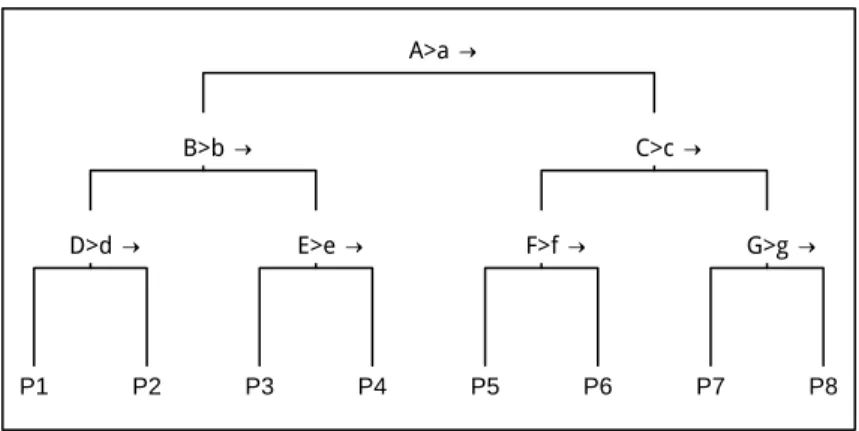
A classification tree introduced in Breiman et al. [17] is a series of splits which partition the predictor space (Rd). Figure 1.1 provides a small example. In the figure, capital letters refer to predictors and lower case letters refer to thresholds. The tree starts at the top; the first partition sends observations with A > ato the right and all others to the left. At the second level, both partitions are split again. The left partition is split so that observations with B > b are sent to the right and the remainder are sent to the left. Likewise, the right partition is split with variable C. The recursive partitioning continues for a prespecified number of levels. In Figure 1.1, the tree has 8 terminal groups labeledP1,P2, etc.
A classification tree is constructed so that the terminal groups are homogenous in terms of the outcome. There are two phases to the tree’s construction: growing and pruning. During the iterations of the growing phase, the algorithm selects a predictor variable and threshold which minimizes variance in the resulting groups. During the pruning phase, splits are eliminated which fail a complexity-benefit criterion.
P1 P2 P3 P4 P5 P6 P7 P8
Figure 1.1: Example of classification tree
calculating the proportion ofy= +1 outcomes in the group. The estimates are plugged into the Bayes rule to generate the classification rule. Because of the sequential nature of selecting splits, trees are sensitive to the earliest splits. Errors because of outliers are perpetuated. This instability is a drawback of the classification tree.
Random forests
Random forests [16] are an ensemble method: a single classifier is constructed by averaging the predictions of several single trees. The individual trees are constructed with a slight modification from before. Rather than considering all predictors as candidates for a split, only a random subset of predictors are considered. A new random subset is selected at each opportunity to make a split. The trees are not pruned.
Thus, if ˆPk(y = +1|x) is thekth random tree generated, then the random forest
(RF) estimate is
ˆ
PRF(y= +1|x)=
1 B
B
X
k=1
ˆ
Pk(y= +1|x).
instability issues inherent in single trees. Also, the sharp divisions between partitions in a single tree are smoothed in a random forest. Lastly, the random forest classifier outperforms a single tree [16].
There are several tree-specific missing data methods, along with EM and im-putation. Any single tree missing data method can be applied to random forests. The tree-specific methods are described in [9, 31, 50]. The following descriptions are summarized from those references.
Surrogate split
Consider the step of selecting a split in the tree. Each predictor is considered individually; if a predictor value is missing, then the observation is momentarily omitted in computations related to the threshold and homogeneity of the outcome. Once the best predictor-threshold split is selected, the algorithm determines a sequence of predictors-thresholds which best replicate the first choice. The sequence is ordered by the quality of the replication. Thus, each split is represented by a sequence of predictor-thresholds, (B < b,E < e, . . . ,W < w), instead of just one. At the moment of classification, an observation is directed to the left or right partition based on the first applicable predictor-threshold pair.
Probability split
weights are naively calculated. The weight in the right partition is the proportion of observed observations in the right partition, likewise for the left weights.
Missing category
In the case of a nominal categorical predictor with missing values, missing is treated as a category. In the case of ordinal data, both discrete and continuous, missing values are replaced with a large value far outside the normal range of values. This allows the algorithm to create partitions which separate missing and non-missing observations. Of course, this strategy can be sensitive to replacing missing values with a large positive value or a large negative value.
A simulation study [31] compared single-tree performance of these three tree-specific methods (with caveats for surrogate split) along with mean imputation and complete case. The probability split performed well in situations when the validation set did not have missing values. The missing category worked well in situations when the missingness mechanism was a function of the outcome y. This is not surprising because the missing category can capture that relationship well.
1.3.4 k-nearest neighbor
The methods presented up to this point have all approached the classification task via a distribution, either by explicitly assuming a distribution (logistic, LDA, and QDA classifiers) or by estimating a distribution (tree-based classifiers). In this section, we consider the nearest neighbor classifier which does not necessarily assume or estimate a distribution.
vision tasks [50], and is especially useful when the probability of group membership changes abruptly at the boundary. Further, because KNN does not require any distri-butional assumptions, it can be applied in nearly any situation. However, the resulting model is not easily interpreted, and calculating distances in large databases requires considerable memory.
Imputation is the most prevalent missing data method for KNN classifiers [2]. KNN itself is used widely as an imputation technique [51], and it has been widely used. Missing values xm
i are predicted from KNN applied to xoi. Say for k = 5, the
replacement ofxm
i is the average of the 5 other training values closest toxoi. In multiple
imputation setups, replacement values are drawn from the set of nearest neighbors.
1.4 Support Vector Machines
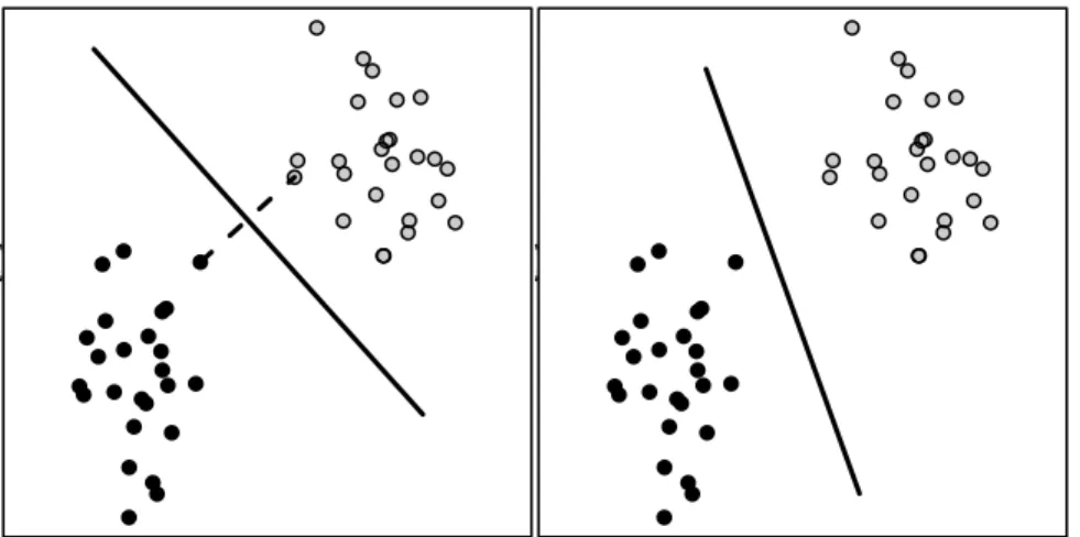
As noted earlier, SVMs are a statistical learning classifier introduced in Boser et al. [15], Cortes and Vapnik [25] and Vapnik [106]. The method has historical basis in linear separating hyperplanes, and the following description builds on that basis. For the sake of demonstration, suppose that thatxis two-dimensions, and that we can plot the data as in Figure 1.2. In this case, the two groups are separable in the sense that there is a lines (planes in higher dimensions) in thex−space which separates the groups. In fact there are infinitely many such lines; two are shown in the figure. Such lines can be used as classifiers for future, unseen points by labeling points on one side of the line as+1 and labeling the others as−1. If we parametrize each line as
{x|wxx+b =0},
then the classifier is f(xo)=sign(wtxo+b), and the signed distance between a pointxo
and the line is||w||−1(wtx
● ● ● ● ● ● ● ● ● ● ●● ● ● ● ● ● ● ● ● ● ● ● ● ● ● ● ● ● ● ● ● ● ● ● ● ● ● ● ● ● ● ● ● ● ● ● ● ● ● X[,2] ● ● ● ● ● ● ● ● ● ● ●● ● ● ● ● ● ● ● ● ● ● ● ● ● ● ● ● ● ● ● ● ● ● ● ● ● ● ● ● ● ● ● ● ● ● ● ● ● ● ● ● ● ● ● ● ● ● ● ● ●● ● ● ● ● ● ● ● ● ● ● ● ● ● ● ● ● ● ● ● ● ● ● ● ● ● ● ● ● ● ● ● ● ● ● ● ● ● ● X[,2] ● ● ● ● ● ● ● ● ● ● ●● ● ● ● ● ● ● ● ● ● ● ● ● ● ● ● ● ● ● ● ● ● ● ● ● ● ● ● ● ● ● ● ● ● ● ● ● ● ●
Figure 1.2: SVM Demonstration, toy data
distance from the line to the nearest point,
margin(w,b)=min
i ||w|| −1|wtx
i+b|.
The motivating, geometric interpretation of a linear SVM is to select the line, of all separating lines, which maximizes the margin. This can be expressed as
min
w,b ||w|| such that yi(w tx
i +b)≥1, i=1, . . . ,n.
misclassified. Specifically,
min
w,b ||w||
+C
n
X
i
ξi
such that yi(wtxi+b)≥1−ξi i=1, . . . ,n (1.5)
ξi ≥0 i=1, . . . ,n.
Thus, in the unseparable case, some points will always incur a penalty because the definition of unseparable implies yi(wtxi+b)<0 for at least one point for everywand
b. The parameterC controls the tradeoffbetween the penalty and the complexity of the classifier. Maximization of the SVM is a quadratic programming problem which can be expressed as
min α
n
X
i=1
αi−
1 2
n
X
i=1
n
X
j=1
αiαjyiyjxtixj
such that 0≤αi ≤C n
X
i=1
αiyi =0,
where the solution isw =Pni=1αiyixi. The key contribution of Cortes and Vapnik [25]
was to identify that the dataxi enters the objective function through the dot-product
xt
ixj, and that general forms of dot-products in a Hilbert space,φ(xi)·φ(xj)=κ(xi,xj),
could replace the euclidean dot-product without affecting the computational burden. General dot-product forms represent a large family of transformations on the data, φ(xi), but they only enter into the computation via a kernel functionκwhich satisfies
certain conditions. Such transformations admit flexible, non-linear functions of the form
f(x)=b+ X
xi∈Tn
This important link between the geometric beginnings of SVM and the kernel trans-formation recast the method into a framework of empirical risk minimization within a Reproducing Kernel Hilbert Space (RKHS) of functions. To see the connection, return to (1.5) and rewrite (wtx
i+b) as f(xi)
min
f∈H ||f||+C n
X
i
ξi
such that ξi ≥1−yif(xi) i=1, . . . ,n
ξi ≥0 i=1, i=1, . . . ,n.
Allow Lh[yi, f(xi)] = max[0, 1−yif(xi)], and the objective function is identical to the
following objective:
fsvm =arg min f∈H λ||f||
2
H
|{z}
penalty
+ RLh,D(f)
| {z }
empirical h-risk
, (1.7)
empirical h-risk: RLh,D(f)= 1 n
n
X
i
max[0, 1−yif(xi)]
| {z } Lh
.
which in an empirical and regularized approximation of the Bayes objective function,
fbayes(x)=arg min
f RLc,P(f).
Asymptotic properties
The SVM solution is unique, stable, consistent, and ensures generalization [94, 98, 34, 50]. Consistency is defined in the statistical sense that finite sample h-risk converges in probability to the minimum h-risk asngets large.,
RLh,P(fsvm)
p
→min
f RLh,P(f).
Generalization refers to fact that the training risk converges in probability to true risk,
RL,D(fsvm) p
→ RL,P(fsvm),
and it suggests that the SVM solution does not over-fit the data as a non-regularized empirical risk solution would.
Steinwart and Christmann [98] and Schölkopf and Smola [94] discuss a number of computational advantages to this setup. The h-loss function seen in equation (1.7) is convex, which allows the implementation of efficient optimization algorithms. As noted above, the SVM solution converges in probability to the minimum h-risk; however, the primary goal is to find a solution that minimizes the c-risk. In fact, as n→ ∞, classification risk of fsvmconverges to the Bayes risk,
RLc,P(fsvm)→min
f RLc,P(f).
Kernel function and tuning parameters
The RKHSHis characterized by a kernel functionκ:Rd×Rd →R, and functions inH are of the form in equation (1.6), and are a linear combination of basis functions hi(x) = κ(x,xi). Computationally, the construction of fsvm(x) centers on finding values
forc1, . . . ,cn andb. Predictions from the SVM classifier are calculated as sign[fsvm(x)].
common choices ofκare
κ(u,v)=utv
| {z }
Linear kernel
and κ(u,v)=e−γ||u−v||2
| {z }
Guassian kernel
.
The linear kernel generates decision rules with a linear boundary; the Gaussian kernel generates both linear and nonlinear boundaries. The details regarding the inherent transformation of Gaussian kernel functions is discussed in Steinwart and Christmann [98].
Note that equation (1.7) includes the parameterλand the definition of the Gaus-sian kernel function includes parameter γ. These parameters are tuning parameters. The cost parameterλ(also reparameterized asC) controls the impact of the complexity penalty relative to the empirical h-risk; the parameterγis a scale or bandwidth param-eter. In practice, the values of tuning parameters are selected from a list of potential values on the basis of cross validation.
Computational details
Equation (1.7) can be re-expressed as a constrained quadratic programming problem forn-vectorα:
min α
1 2α
tW
α−1tα (1.8)
such that ytα=0
0≤αi ≤C, i=1, . . . ,n
Note the conventions: (a)1is a vector of ones, (b) C = 1/(2λn), (c) the kernel matrix
Kij = κ(xi,xj), and (d)Wij = yiKijyj. With optimalα, the SVM classifier is defined in
equation (1.6) withci = yiαi. One result of the computation is thatαi =0 for
component of the classifier in equation (1.6) can be omitted. Only those observations inside the margin, yif(xi) ≤ 1, contribute to the classifier and are call ‘the support
vectors’. As such, the SVM solution represents data reduction in the sense that all non-support vectors can be omitted from the training set without affecting the resulting classifier. This, especially in large databases, is an advantage of the SVM model.
A wide variety of computational algorithms exist for solving this quadratic programming problem; most SVM software packages implement a type of sequential minimal optimization (SMO). This specific algorithm can solve (1.8) even when the memory required for then×nmatrixWexceeds available computer memory; thus, the SMO algorithm can generate a solution when the sample size is large. For a discussion of computational details see [20, 94].
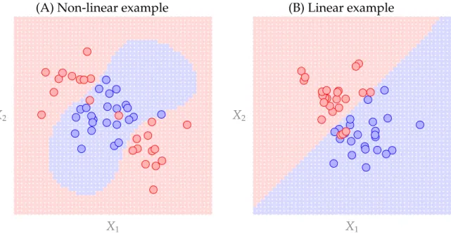
SVM example with toy data
(A) Non-linear example (B) Linear example
X1
X2
X1
X2
Figure 1.3: Examples of Two SVM Classifiers
Panel (A) is a non-linear example fit with Gaussian kernel; panel (B) is a linear example fit with linear kernel. Training set data is plotted as larger, darker circles. The regions defined by the SVM classifier are denoted with the red or blue background colors. The tuning parameters selected with cross validation areC=0.125.
SVM methods for missing data
Improper Imputation
suggests an imputation scheme in which parameters of the imputation distribution are jointly selected with the classification function. That is, it searches for the classifier and the missing data distribution which minimizes loss. The performance of the method is compared to single imputation with MCAR missing data. On balance, results comparing this imputation method to single imputation showed 1% - 2% improvement in accuracy, though some example datasets showed around 4% improvement.
Kernel Completion
Kernel completion is an SVM specific missing data method suggested in Tsuda et al. [100] and Anderson and Gupta [3]. The method centers on equation (1.8), the quadratic programming problem which solves the SVM objective function. Note that data from the predictors xi enter the expression solely through the kernel matrix K.
Thus, when the outcomes yi are fully observed and missing data is restricted to the
predictors, the kernel completion method for missing data is to reconstructK. WithK
in hand, a solution forcisin (1.6) is available. WhenKis the linear kernel, no additional
steps are needed. WhenKis a non-linear kernel, one must also specifyκ(x,xi) in the
same equation.
In Tsuda et al. [100], authors propose a kernel completion method in which one uses auxiliary information to fill-in the missing portions of the kernel matrix. The argument goes something like this: LetPbe the partially observed kernel matrix. Let
Mbe a kernel matrix derived from fully observed auxiliary data. Think of Pand M
as covariance matrices from zero mean multivariate normal distributions. Then, the Kullback-Leibler distance is
KL(P,M)=tr(M−1P)+log detM−log detP−n
in a way that (a)Premains positive semi-definite and (b) minimizesKL(P,M). Because this method assumes an auxiliary data set, it is only applicable to situations when such data is available and when one can argue that the auxiliary data is a reasonable surrogate. Thus, this method is quite limited in its application.
In Anderson and Gupta [3], researchers proposed kernel completion method in which one specifies distributions for the predictor vectorxi and then calculates the
expected kernel,
E[Kij]=
Z Z
κ(xi,xj)p(xi)p(xj)dxidxj.
The authors are not clear if the assumed distributions should be conditional on the observed components. This framework is similar to multiple imputation methods: rather than averaging several classifier functions, one averages several kernels and then finds a single classifier. Like imputation, this method is easy to implement. But like imputation, it relies on convenience distributions.
Missing data loss function
Smola et al. [97] provides a principled missing data method based on a connec-tion between SVM and exponential family distribuconnec-tions. Specifically, if 2yφ(x) is the sufficient statistic ofp(y|x), then the SVM solution with kernelκ(xi,xj)=φ(xi)·φ(xj) is
also the solution which maximizes the log-likelihood ratio. The method proposes that for missing data, one replace the loss function with one constructed with sufficient statistics from the distributionp(y|xo). The solution requires a number of “thorny” [97] computational issues, and it is limited in workable size.
Probability Constraint
missing data method in which the first constraint is replaced by a probability statement:
P(1−yif(xi)≤ξi|xoi,yi)≥1−vi vi ∈(0,1]; i=1, . . . ,n.
In essence, this method replaces uncertain observations with distributions. Think-ing geometrically, the standard constraint penalized each misclassified point. The probability constraint penalizes uncertain points if 1−vi percent of the distribution
is misclassified. The computation of this solution is non-trivial especially with any non-linear kernel. In the case of the linear kernel, the resulting objective function is a second order cone program. This limits the solvable sample size and increases computation time. The computational issues are exacerbated in the case of non-linear kernels like the Gaussian. Despite the computational issues, the probability constraint method is applicable to MCAR and MAR missing data situations.
Geometric Max Margin
Chechik et al. [22] proposed a missing data method built on the geometric perspective of SVMs; the basic idea is to define the margin in terms of non-missing predictor variables. That is, to define the margin within a subspace. Recall that the geometric linear SVM objective function is
max
w,b mini ||w|| −1
|wtxi+b|
| {z }
margin
.
The geometric max margin method redefines the margin uniquely for each observation. If ri is the indicator vector (as defined in section 1.2.3) then the margin within the
observed subspace is
margin(w,b,xi,yi)=
d
X
k=1
rikw2k
−1
b+
d
X
k=1
wkrikxik
and the objective function is
max
w,b mini margin(w,b,xi,yi).
This geometric solution performs reasonably well when the missing data are MCAR, but it does not work well when the missing data are MAR. Further, the computation requires non-convex optimization when the two groups are not separable. This limits the computational speed and the size of the training set.
1.5 Multi-class Support Vector Machines
Due to the popularity of SVMs in the two-class setting, a natural extension of the method is the multi-class setting in which one wants to construct a classifier that distinguishes between more than two classes. There are two families of multi-class SVMs, which we consider in turn.
1.5.1 Composite-of-binary SVMs
is constructed so that one potential class is eliminated at each decision node, and the terminal node represents the class prediction. Lastly, we describe the one-versus-many classifier which generatesKbinary rules which separate generic classifrom all other classes. To classify a point, the covariate vector is input to each two-class rule; the final prediction corresponds to the class which generated the largest signed distance, i.e.,
ˆ
y = arg maxi=1,...,K fi(x). Variations of the these composite-of-binary SVMs exist, and
generally vary by how each component classifier casts a vote for a potential class. For example, using the component SVMs to generate probability estimates which in turn are combined in a final decision rule. See [49, 80, 20, 110] for a discussion of generating and combining multi-class probabilities from SVMs.
1.5.2 Simultaneously Trained SVMs
The second family of multi-class SVM builds a decision rule by simultaneously trainingKfunctions where each function corresponds to a single class [107, 26, 62, 69]. Distinguished by specific multi-class loss functions, the various flavors of multi-class SVMs simultaneously construct theKfunctions so that the predicted class corresponds to the function with the largest value. The simultaneous estimation of theKfunctions ensures that the estimated multi-class rule targets the multi-class Bayes rule.
The general setup is very similar to the two-class setting, and we describe it here. Consider a training set, Tn, ofn observations, each consisting of a d-vector of
covariates,x ∈ Rd, and multi-class outcome, y ∈ {1, . . . ,k}. Each observation is an iid draw from an unknown distributionP(x,y). Consider functionsf(x)={f1(x), . . . , fk(x)}
so that the class label ofxcan be predicted as
ˆ
y=arg max
i fi(x).
The classifier which minimizes the average classification error overP(x,y) is the Bayes classifier,
fbayes=arg min
f EP[y
,arg max
i fi(x)].
The average classification error of the Bayes classifier is called the Bayes risk. The goal is to construct a classifier from the training setTnwhich is asymptotically a Bayes
classifier but also performs well in finite sample situations.
The SVM solution frames the task within empirical risk minimization; specifi-cally, the SVM solution is
ˆ
f=arg min
f∈H λ||f||
2
H +
1 n
n
X
i=1
such that
k
X
i
fi(x)=0
where||f||H = Pki ||fi||2H and L[yi,f(xi)] is a loss function which penalizes
misclassifica-tion. The multi-class SVM methods discussed here build on the reinforced multi-class SVM (RMSVM) proposed in [69] because it provides a multi-class loss function which unifies the earlier work of [62] and [107] as special cases of a general multi-class loss function. The RMSVM loss function is
L[y,f(x)]=γ[(k−1)− fy(x)]++(1−γ)
X
j,y
[1+ fj(x)]+
where the function [t]+ = max{0,t} and γ is a tuning parameter which calibrates the
loss. The set of solutions,H, is constructed so that each component of solution, ˆf, is of the form
fi(x)=b+ n
X
j=1
cjK(x,xj) xj ∈ Tn
whereK(u,v) is a kernel function. The linear kernel,K(u,v) = utv, and the Gaussian
kernel,K(u,v)=exp{−σ||u−v||2}, are commonly used.
As the solution to the empirical risk minimization problem, the SVM targets the conditional expectation of the loss function, E{L[y,f(x)]|x}. When γ ≤ 1/2, the RMSVM solution is Fisher consistent in the sense that the minimizer ofE{L[y,f(x)|x]}is also the multi-class Bayes rule [69]. Simulation examples in [69] show that the RMSVM performs better whenγ =1/2 than whenγ=0 or 1.
1.6 Semi-supervised Learning and Support Vector Machines
immunohistochemistry data, or data for which disease subtype must be ascertained by biopsy or expensive blood-assay, as with rare forms of hepatitis. Often, the research goals associated with these types of datasets is to construct a classifier which predicts class labels because the gold-standard method is inaccessible. Classifiers built with some missing class labels are often called semi-supervised classification rules [87].
There are existing methods for constructing semi-supervised two-class or multi-class rules in statistical learning contexts, many of which are based on missing data ideas like imputation and the expectation-maximization (EM) algorithm while other methods are based on statistical learning ideas like boosting. For example, [42] ap-plied EM as a way to estimate Gaussian mixture models in an unsupervised, clustering context and to missing data in a supervised context. In [76], researchers perform semi-supervised text classification with a naive Bayes classifier and the EM algorithm. Imputation type semi-supervised classification include co-training [14] and ASSEM-BLE [12]. In [103], authors provide a general purpose semi-supervised algorithm for any multi-class classifier based on boosting.
1.6.1 S3VM
One semi-supervised method specific to two-class SVMs is the method intro-duced in [11] called S3VM. While standard SVM methodology chooses the rule which
minimizes the empirical hinge risk, S3VM chooses the rule which minimizes the
em-pirical hinge risk calculated as if unlabeled points are in fact correctly labeled. Because unlabeled points are treated as correctly classified, the unlabeled points in the empir-ical hinge risk act as a ‘high density’ penalty. That is to say, the S3VM setup prefers
rules with boundaries in low density regions. Computationally, the S3VM objective
function is not convex and has potentially many local minima; however, there are a number of algorithms developed to find the S3VM solution. See [118, 117, 21] for a
for constructing S3VM rules.
Multi-class extensions of S3VM were proposed in [113] for specific types of
kernels (sparse and full rank) with a specific multi-class loss function. Using a sparse Laplacian kernel matrix (a kernel to which the method applies), the algorithm employs gradient descent to find a solution. In contrast to the limited setting of sparse and full rank kernels, a more accessible multi-class extensions of S3VM have been developed
with the composite-of-binary multi-class SVM, such as the methods proposed first in [21] and adapted in [6]. In [21], the composite-of-binary multi-class SVM applies S3VM methods to each of the two-class rules. The method requires all unlabeled
points to be included when training each two-class rule, even with a one-versus-one rule. In [6], authors adapted the composite-of-binary S3VM method of [21] by
intro-ducing participation weights of unlabeled observations. Based on a generic similarity measure, the participation weights will up-weight or down-weight the contribution of unlabeled observations when training individual two-class S3VMs as part of the
larger composite-of-binary rule. Thus, unlabeled observations which are similar to class 1 observations are given greater weight when constructing rules involving class 1. Likewise, observations not similar to class 1 are given less weight. As demon-strated in a number of examples, using participation weights in the construction of semi-supervised composite-of-binary multi-class SVMs appears to improve classifier performance.
1.6.2 Maximum Margin Clustering
found, an SVM classifier is constructed from a training set composed of the new class labels and covariates. The key extension of max margin clustering to semi-supervised learning is that the max margin clustering objective function can incorporate informa-tion from observainforma-tions with known outcomes by introducing constraints. Often called the semi-definite SVM (SD-SVM) because the objective function is a semi-definite pro-graming problem, the SD-SVM is similar to S3VM in the two-class setting but has
the additional advantage of also providing a multi-class solution. However, the SD-SVM as a semi-supervised method is limited in application by the computationally expensive algorithm, its sensitivity to tuning parameters, and its assumption that the intercept term (sometimes called the bias term) is zero [102]. While [102, 116] pro-posed unsupervised clustering algorithms based on SD-SVM which minimize these drawbacks, the resulting methods do not admit a semi-supervised solution.
The SD-SVM can be framed as a two-step procedure in which the first step clusters the data and the second step constructs an SVM based on the predicted class labels. A cluster-then-construct solution is one in which any clustering procedure provides class labels in the first step and an SVM is constructed in the second step. SD-SVM differs from this ad-hoc procedure because the clustering criteria minimized in the first step is the SVM empirical risk. Note that the semi-supervised composite-of-binary multi-class SVM from [6] which is described above is another flavor of the cluster-then-construct type solution. The first step generates fuzzy-cluster labels in the form of participation weights and the second step constructs a composite-of-binary, one-versus-one S3VM rules. Because this method relies on a composite-of-binary SVM,
its computational burden is much less than SD-SVM.
SVMs has been questioned, as a number of authors have provided examples where complete-case multi-class SVMs out perform semi-supervised multi-class SVMs, such as [120] and [63]. Further, the computation required for many semi-supervised meth-ods can be substantial, though recent algorithms such as those described in [96] im-prove on earlier algorithms for two-class SVMs. In the multi-class setting, however, computation time may still be prohibitively expensive, such as the SD-SVM solution which requires estimation of n+ n2
u parameters where n is the number of
observa-tions andnuis the number of unlabeled observations. Multi-class methods which are
computationally expensive like the multi-class S3VM methods are restricted to specific
application areas (sparse, full rank kernels) or rely on composite-of-many SVMs. In our judgment, there is a need for a stable, multi-class semi-supervised SVM.
1.7 Dissertation topics
The missing data methods for SVMs, with a few exceptions, are ad-hoc tech-niques. Those that are based on statistical reasoning are limited in sample size, only apply to MCAR missing data, or require specialized software. In the first paper, we will propose an EM-type missing data method which can be performed with standard SVM software. As such, this method will provide SVM users an important tool to address a common issue. The performance of the method is examined in a simula-tion study and in applicasimula-tion to a subset of an observasimula-tional study database of patients treated for hepatitis C (HCV-TARGET). The simulations cover a variety of missing data scenarios, including situations in which missingness in the covariates is a function of the outcome.
solution requires estimation of data distribution parameters, and in high dimensional settings, the number of parameters can be very large. Second, for missingness in continuous covariates, it requires MCMC methods for sampling from the conditional EM distribution which can be time consuming. Thus, as the method developed in the second paper avoids these issues, it may be particularly helpful for high dimensional settings, a common setting for SVMs.
CHAPTER 2: AUGMENTED AND WEIGHTED SUPPORT VECTOR MACHINES FOR MISSING COVARIATES
2.1 Introduction
Hepatitis C is the most prevalent blood born infection in the United States [24] with 3.4 to 4.9 million infected US residents [5]. The mortality burden of hepatitis C continues to grow, and in 2007 the number of deaths from hepatitis C exceeded those from HIV [71]. In the last five years, new drug therapies such as Telaprevir have offered physicians an effective means for treating hepatitis C infection [1]. How-ever, the cost of these new treatments is substantial. In the United States, the cost per cure for Telaprevir ranges between $150,000 and $250,000 [101]. The prevalence of hepatitis C infection coupled with the cost of treatment are motivating factors for developing classification rules that identify patients which are more likely to respond to treatment. Such rules could improve the cost effectiveness of treatment and lower the risk of unnecessary therapy. HCV-TARGET is a multi-center longitudinal obser-vational study which enrolls a diverse population of patients receiving treatment for hepatitis C. Researchers collected relevant demographic, clinical, and outcome data during treatment and follow-up. A scientific objective is to develop a classifier that can accurately predict treatment efficacy using baseline variables.
analysis [83], and other biomedical computer vision tasks. SVMs represent a natural approach for building a decision rule because of the modeling flexibility. However, SVMs do not easily accommodate missing covariate information, yet this is of prime importance within the HCV-TARGET study as the researchers were unable to collect all baseline data for all patients for a wide variety of reasons. For example, physicians sometimes collected certain chemistry measures and not others depending on the pa-tient’s health or the presence of comorbidities. In other instances, the cause of missing baseline chemistry measures is unknown. It is necessary to accommodate the missing data in developing SVM based classifiers.