STATISTICAL METHODS FOR THE ANALYSIS OF MULTI-OMICS AND MULTI-STUDY DATASETS
Sean McCabe
A dissertation submitted to the faculty of the University of North Carolina at Chapel Hill in partial fulfillment of the requirements for the degree of Doctor of Philosophy in the Department of Biostatistics
in the Gillings School of Global Public Health.
Chapel Hill 2020
ABSTRACT
Sean McCabe: Statistical Methods for the Analysis of Multi-Omics and Multi-Study Datasets (Under the direction of Dr. Michael I. Love and Dr. Danyu Lin)
The generation of multiple, large scale genomic datasets has become increasingly common in biological and biomedical research. These datasets can be collected for a common set of samples over multiple assays, known as a multi-omics dataset, or for the same assay over multiple collections of samples, known as a multi-study dataset. The growth of multi-omics datasets has given rise to many methods that identify sources of common variation across data types. However, the unsupervised nature of these methods makes it difficult to evaluate their performance. We propose Multi-Omics VIsualization of Estimated contributions (MOVIE), to evaluate the extent of overfitting of multi-omics methods. MOVIE utilizes a cross-validation approach to identify method stability and provides a visualization of the overfitting. Plotting the contributions of one data type against another produces contribution plots, where contributions are calculated for each subject and each data type from the results of each multi-omics method. The usefulness of MOVIE is demonstrated through evaluating the performance of multi-omics methods on large and small-sample experimental datasets and identifying overfitting in a permuted null dataset.
Genotype-Tissue Expression (GTEx) project as a reference dataset, we evaluate ACTOR on simulated and real RNA-seq datasets to determine tissue-type classifications of genes.
ACKNOWLEDGEMENTS
First, I would like to express my deepest gratitude to my advisors, Dr. Michael Love and Dr. Danyu Lin, for their support, advice, and patience. Their guidance throughout my time at the University of North Carolina at Chapel Hill has been invaluable and I am forever grateful for the time I spent working as their student. Through working with them, I have developed my research skills, pursued topics for which I have a passion for, and further solidified my statistical understanding.
I am also very thankful for Dr. Joseph Ibrahim. From the very beginning, he has given me many opportunities which I am very grateful for. His continued support and mentorship have helped me develop as a statistician. Many thanks to my committee members Dr. Andrew Nobel, Dr. Naim Rashid, and Dr. Terry Furey for serving on my committee and for providing helpful comments on my research. Their detailed insights have greatly improved the quality of this work.
TABLE OF CONTENTS
LIST OF FIGURES . . . ix
CHAPTER 1: LITERATURE REVIEW . . . 1
1.1 Multi-Omics Methods . . . 1
1.1.1 PC-CCA . . . 2
1.1.2 Sparse mCCA . . . 3
1.1.2.1 Tuning Parameter Selection . . . 4
1.1.3 AJIVE . . . 4
1.1.4 MOFA . . . 5
1.1.5 Current Comparisons of Multi-Omics Methods. . . 6
1.1.6 Summary . . . 6
1.2 Multi-Study Datasets . . . 7
1.3 Isoform Splicing . . . 7
1.3.1 Differential Transcript Usage . . . 7
1.3.2 DRIMSeq . . . 8
1.3.3 DEXSeq . . . 9
1.3.4 SUPPA2 . . . 9
1.3.5 Genomic Reference Panels . . . 10
1.3.6 Distances on Isoform Proportions . . . 11
1.3.7 Topic Modeling - LDA . . . 12
1.3.8 Summary . . . 15
1.4 Sample Quality Weighting . . . 15
1.4.1 Weighting Methods . . . 15
1.4.3 Summary . . . 17
CHAPTER 2: MOVIE - MULTI-OMICS VISUALIZATION OF ESTIMATED CONTRIBUTIONS 19 2.1 Framework for Evaluation of Methods . . . 19
2.1.1 Contributions . . . 20
2.1.2 Cross-validation . . . 21
2.1.3 Multi-omics Datasets . . . 24
2.2 Evaluation of Methods . . . 27
2.3 Discussion . . . 29
CHAPTER 3: ACTOR - A LATENT DIRICHLET MODEL TO COMPARE EX-PRESSED ISOFORM PROPORTIONS TO A REFERENCE PANEL . . . 31
3.1 ACTOR . . . 31
3.2 Variational Bayes Estimation and Implementation . . . 36
3.3 Results . . . 38
3.3.1 GTEx and Data Processing . . . 38
3.3.2 Simulated Data . . . 39
3.3.3 Spinal Cord RNA-seq Data . . . 43
3.4 Discussion . . . 45
3.5 Software Availability . . . 46
CHAPTER 4: SQWCCA - SAMPLE QUALITY WEIGHTED CANONICAL COR-RELATION ANALYSIS . . . 47
4.1 Model . . . 48
4.2 Model Fitting . . . 50
4.3 Weighted Matrices . . . 50
4.4 Estimating Tuning Parameters . . . 52
4.5 Data Preparation . . . 53
4.5.1 Simulations on TCGA data . . . 53
4.5.2 Crohn’s disease and non-IBD . . . 55
4.6.1 Simulations on TCGA data . . . 55
4.6.2 Crohn’s disease and non-IBD . . . 57
4.7 Discussion . . . 59
CHAPTER 5: CONCLUSION . . . 61
APPENDIX A: SUPPLEMENTARY MATERIALS FOR MOVIE . . . 63
A.1 Large Sample Size - TCGA Data . . . 63
A.2 Small Sample Size - Li et al, 2016 . . . 72
A.3 Permuted Null Data . . . 80
APPENDIX B: SUPPLEMENTARY MATERIALS FOR ACTOR . . . 82
B.1 Supplementary Tables . . . 82
B.2 Supplementary Methods . . . 82
B.2.1 Variational Inference. . . 82
B.2.2 Estimation ofφ. . . 86
B.2.3 Estimation ofλ. . . 86
B.2.4 Estimation ofη. . . 87
B.2.5 Estimation ofρ. . . 88
B.2.6 Estimation ofβ. . . 89
B.3 Supplementary Figures . . . 90
APPENDIX C: SUPPLEMENTARY MATERIALS FOR SQWCCA . . . 103
C.1 Notation . . . 103
C.2 Derivative of Objective Function . . . 104
C.3 Supplementary Figures . . . 107
LIST OF FIGURES
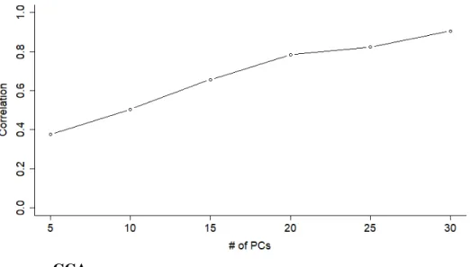
1.1 CCA on PCs of null Gaussian data returns correlations as high as 0.9, for
datasets of sizes that are typical genomics (e.g. 100 samples, 5000 genes). . . 3 2.2 Each method shown in the figure generates a set of weights for each data type.
Our analysis only considers the first set of weights to avoid issues related to a
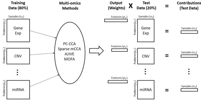
potentially complex set of mappings of factors across data splits. . . 21 2.3 Pipeline for cross-validation analysis. Training Data: Dataset is subset to
80% of the original data and will be used to train the model. Multi-omics Methods: The training data are analyzed using the specified method.Output: Weights are output from the multi-omics methods. Test Data: The remaining 20% of the original data are used as test data and multiplied by the subsequent weights.Contributions: The result of multiplying the output weights by the test set data. Each sample in the test data yields one number that represents the
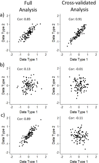
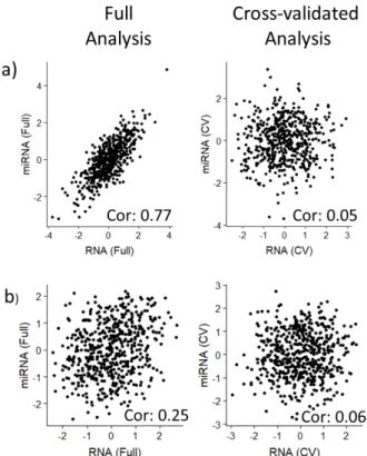
contribution per data type. . . 23 2.4 The figure provides hypothetical scenarios for the contribution plot, generated
using artificial data. a. A strong correlation in both the full and CV plots, indicating that the method accurately fits the data and that the two data types are linearly related.b. A null correlation in both the full and CV plots, indicating that the method did not overfit and that the two data types are not related in terms of this factor.c. A strong linear relationship in the full plot and a null relationship in the CV plots, indicating that the method overfit and that the two
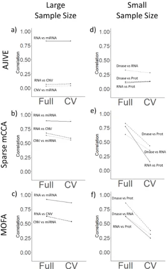
data types are not associated with the top factor. . . 25 2.5 Overfitting plot: Plots of the pair-wise correlations identified in the full and CV
contribution plots for each method. The left column (plots a-c) corresponds to the large-sample analysis (n=558; TCGA breast cancer), while the right column (plots d-f) corresponds to the small-sample size analysis (n=53; Li, et al 2016) . Rows correspond to AJIVE, Sparse mCCA, and MOFA, respectively. Flat lines indicate non-overfitting methods, while lines with a negative slope
indicate a large change in the results for the full and CV plots. . . 26 2.6 Side-By-Side contribution plots fora)PC-CCA with 100 PCs andb)Sparse
mCCA with the null dataset: Left panels show the contribution plots from the full analysis, while right panels show the contribution plots for the CV analysis.
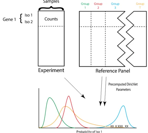
Pair-wise correlations are reported on the figure. . . 29 3.7 ACTOR uses precomputed Dirichlet parameters for each reference group to
identify which reference group a set of experimental samples is most similar to based on isoform splicing patterns. The curves represent the Dirichlet distribution for each reference group. ‘X’ corresponds to an experimental
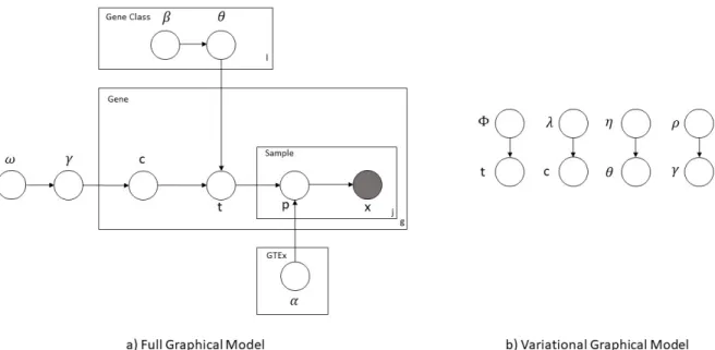
3.8 Graphical model representation of our proposed framework. Figure a) cor-responds to the full model while Figure b) corresponds to the variational
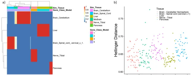
distribution. . . 34 3.9 a) Multinomial posterior estimates for the probability vector for tissue
mem-bership (φ) using a simulated dataset of 50 samples fitting the model with ten gene classes. Annotation bars above the figure represent the tissue that was simulated and the gene class that was identified by the model. Columns are genes and rows are the GTEx tissues. b) Hellinger distance between a random sample of GTEx and a simulated experimental dataset. Points are for each GTEx sample and correspond to the average Hellinger distance between that
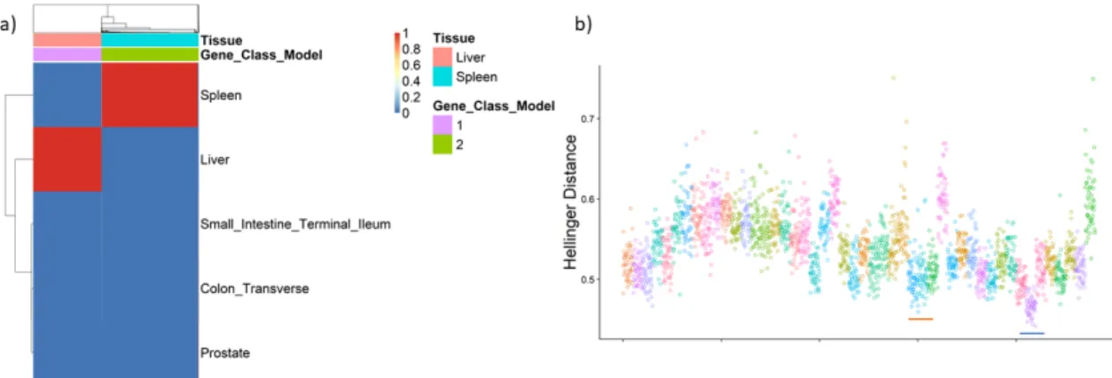
sample and each experimental sample. . . 40 3.10 a) Posterior estimates for the probability vector for tissue membership (φ)
using a dataset of 100 samples generated from a mixture of GTEx liver and spleen tissues. Annotation bars above correspond to the simulated tissue and the gene class identified by the model. b) Hellinger distance between a random sample of GTEx and a simulated experimental dataset containing spleen and liver genes. Points are for each GTEx sample and correspond to the average Hellinger distance between that sample and each experimental sample. The red bar identifies the liver GTEx samples and the blue bar identifies the spleen
GTEx samples. . . 42 3.11 a): Posterior estimates for the probability vector for tissue membership (φ)
using a real dataset of 8 motor neuron samples. b): Hellinger distance between a random sample of GTEx and motor neuron samples. Points are for each GTEx sample and correspond to the average Hellinger distance between that sample and each experimental sample. The blue bar identifies the brain GTEx
samples. . . 44 4.12 SQWCCA uses the contributions from Sparse CCA and a Quality Score to
learn sample-specific weights that maximize the correlation between the contributions. . . 49 4.13 Simulation 1: a) Contribution plot for the full analysis and b) plot of the derived
weights by the randomly generated quality score. Dotted line is placed at the
value ofα(-4.34). . . 56 4.14 Simulation 2: a) Contribution plot for the full analysis and b) plot of the derived
weights by the ordered quality score. Red points correspond to samples that
have random RNA-seq. Dotted line is placed at the value ofα(-1.75). . . 57 4.15 Simulation 4: a) Contribution plot for the full analysis and b) plot of the derived
weights by the total read counts. Red points correspond to samples that were
down-sampled. Dotted line is placed at the value ofα(2.18e7). . . 58 4.16 Real Data: a) Contribution plot for the full analysis and b) plot of the derived
weights by the TSS enrichment score. Dotted line is placed at the value ofα (6.61). Red points correspond to the six samples that were identified with low
A.17 Sparse mCCA with experimental data: Side-by-side contribution plots for gene
expression versus miRNA using Sparse mCCA. . . 63 A.18 Sparse mCCA with experimental data: Side-by-side contribution plots for
CNV versus miRNA using Sparse mCCA. . . 64 A.19 Sparse mCCA with experimental data: Side-by-side contribution plots for
CNV versus gene expression using Sparse mCCA. . . 64 A.20 MOFA with experimental data: Side-by-side contribution plots for gene
ex-pression versus miRNA using MOFA. . . 65 A.21 MOFA with experimental data: Side-by-side contribution plots for CNV versus
miRNA in experimental data using MOFA. . . 65 A.22 MOFA with experimental data: Side-by-side contribution plots for CNV versus
gene expression using MOFA. . . 66 A.23 AJIVE with experimental data: Side-by-side contribution plots for gene
ex-pression versus miRNA using AJIVE. . . 66 A.24 AJIVE with experimental data: Side-by-side contribution plots for CNV versus
micro RNA using AJIVE. . . 67 A.25 AJIVE with experimental data: Side-by-side contribution plots for CNV versus
gene expression using AJIVE. . . 67 A.26 Sparse mCCA with experimental data: Comparison plots for CNV, gene
expression, and miRNA using Sparse mCCA. . . 68 A.27 MOFA with experimental data: Comparison plots for CNV, gene expression,
and miRNA using MOFA. . . 68 A.28 AJIVE with experimental data: Comparison plots for CNV, gene expression,
and miRNA using AJIVE. . . 69 A.29 Contribution correlations for AJIVE for each pair of data sets in an analysis
with increased ranks for CNV. . . 69 A.30 Pairwise plots of RNA contributions for a)Sparse mCCA vs. AJIVE, b)
MOFA vs. AJIVE, andc)MOFA vs. Sparse mCCA . . . 70 A.31 Pairwise plots of CNV contributions fora) Sparse mCCA vs. AJIVE, b)
MOFA vs. AJIVE, andc)MOFA vs. Sparse mCCA . . . 70 A.32 Pairwise plots of miRNA contributions fora)Sparse mCCA vs. AJIVE,b)
MOFA vs. AJIVE, andc)MOFA vs. Sparse mCCA . . . 71 A.33 Plot of expression of ESR1 gene against the RNA contribution fora)Sparse
A.34 MCCA with small-sample dataset: Contribution plots for DNase and Protein
expression using MCCA. . . 72 A.35 MCCA with small-sample dataset: Contribution plots for DNase and gene
expression using MCCA. . . 73 A.36 MCCA with small-sample dataset: Contribution plots for protein expression
and gene expression using MCCA. . . 73 A.37 MOFA with small-sample dataset: Contribution plots for DNase and protein
expression using MOFA. . . 74 A.38 MOFA with small-sample dataset: Contribution plots for DNase and gene
expression using MOFA. . . 74 A.39 MOFA with small-sample dataset: Contribution plots for protein expression
and gene expression using MOFA. . . 75 A.40 AJIVE with small-sample dataset: Contribution plots for DNase and protein
expression using AJIVE. . . 75 A.41 AJIVE with small-sample dataset: Contribution plots for DNase and gene
expression using AJIVE. . . 76 A.42 AJIVE with small-sample dataset: Contribution plots for protein expression
and gene expression using AJIVE. . . 76 A.43 MCCA with small-sample dataset: Comparison plots for DNase, protein
expression, and gene expression using AJIVE. . . 77 A.44 MOFA with small-sample dataset: Comparison plots for DNase, protein
ex-pression, and gene expression using AJIVE. . . 77 A.45 AJIVE with small-sample dataset: Comparison plots for DNase, protein
ex-pression, and gene expression using AJIVE. . . 78 A.46 Comparison plots of contributions from Sparse mCCA for the 3 fold analysis. . . 78 A.47 Comparison plots of contributions from Sparse mCCA for the 10 fold analysis. . . 79 A.48 MOFA with null data: Side-by-side contribution plots for miRNA versus gene
expression using MOFA. . . 80 A.49 AJIVE with null data: Side-by-side contribution plots for miRNA versus gene
expression using AJIVE. . . 81 B.50 Toy example of potential gene classes. Columns correspond to gene classes
with each gene class containing a potentially different number of genes. Rows correspond to the groups from the reference panel. Gene class 1 aligns with reference group 1, gene class 2 aligns with reference group 2, and gene class 4 aligns with reference group 5. Gene class 3 is shown to be equally similar to
B.51 Diagram of data generation for Simulation 1. Using the precomputed Dirichlet estimates of the reference panel, a per gene Hellinger distance is calculated on the mean isoform proportion between liver, tibial nerve, spinal cord, cere-bellum, and pancreas tissues. Genes are considered for the simulation from a given tissue if the Hellinger distance to all other tissues is greater than 0.1. Additionally, genes which had a Hellinger distance between the spinal cord and cerebellum tissues less than 0.4 and greater than 0.8 to all other tissues were considered for simulating as a mixture of the two tissues. Gene expression was simulated for all genes using a Negative Binomial distribution withsize= 20
andµ = 200. Isoform expression for each gene was simulated by drawing from a Dirichlet Multinomial conditioned on the fixed total gene expression. In total 350 genes were simulated with 100 from liver, 50 from tibial nerve, 50 from spinal cord, 100 from cerebellum, 25 from pancreas, and 25 from a
mixture of cerebellum and spinal cord. . . 91 B.52 Diagram of data generation for Simulation 2. 50 liver and 50 spleen samples
were randomly selected from the GTEx dataset. A hybrid sample was created by randomly selecting half of the genes with 2-5 annotated isoforms as being liver with the other half being spleen. Genes were then removed if the isoform
patterns were similar across all GTEx tissues. . . 91 B.53 Hellinger distance between a random sample of GTEx and a simulated
experi-mental dataset containing spleen and liver genes. Points are for each GTEx sample and correspond to the average Hellinger distance between that sample
and each experimental sample. . . 92 B.54 Heatmap of the isoform proportions for gene ENSG00000108797.7, which
aligned to amygdala. Each column corresponds to an isoform of this gene with the rows corresponding to either a tissue group from GTEx or an exper-imental sample indicated by the first annotation bar. Cells are the estimated isoform proportions for GTEx tissues and the observed isoform proportions for experimental samples. The second annotation bar shows the posterior estimate from the model for the tissue group membership. The last annotation bar is the inverse precision for the GTEx tissue for this gene. Experimental samples will
not have a value for the last two annotation bars. . . 93 B.55 Heatmap of the isoform proportions for gene ENSG00000122484.8, which
aligned to cerebellar. Each column corresponds to an isoform of this gene with the rows corresponding to either a tissue group from GTEx or an exper-imental sample indicated by the first annotation bar. Cells are the estimated isoform proportions for GTEx tissues and the observed isoform proportions for experimental samples. The second annotation bar shows the posterior estimate from the model for the tissue group membership. The last annotation bar is the inverse precision for the GTEx tissue for this gene. Experimental samples will
B.56 Heatmap of the isoform proportions for gene ENSG00000064419.9, which aligned to liver. Each column corresponds to an isoform of this gene with the rows corresponding to either a tissue group from GTEx or an experimental sample indicated by the first annotation bar. Cells are the estimated isoform proportions for GTEx tissues and the observed isoform proportions for ex-perimental samples. The second annotation bar shows the posterior estimate from the model for the tissue group membership. The last annotation bar is the inverse precision for the GTEx tissue for this gene. Experimental samples will
not have a value for the last two annotation bars. . . 95 B.57 Heatmap of the isoform proportions for gene ENSG00000047932.9, which
aligned to liver. Each column corresponds to an isoform of this gene with the rows corresponding to either a tissue group from GTEx or an experimental sample indicated by the first annotation bar. Cells are the estimated isoform proportions for GTEx tissues and the observed isoform proportions for ex-perimental samples. The second annotation bar shows the posterior estimate from the model for the tissue group membership. The last annotation bar is the inverse precision for the GTEx tissue for this gene. Experimental samples will
not have a value for the last two annotation bars. . . 96 B.58 Heatmap of the isoform proportions for gene ENSG00000101474.7, which
aligned to heart. Each column corresponds to an isoform of this gene with the rows corresponding to either a tissue group from GTEx or an experimental sample indicated by the first annotation bar. Cells are the estimated isoform proportions for GTEx tissues and the observed isoform proportions for ex-perimental samples. The second annotation bar shows the posterior estimate from the model for the tissue group membership. The last annotation bar is the inverse precision for the GTEx tissue for this gene. Experimental samples will
not have a value for the last two annotation bars. . . 97 B.59 Heatmap of the isoform proportions for gene ENSG00000106244.8, which
aligned to heart. Each column corresponds to an isoform of this gene with the rows corresponding to either a tissue group from GTEx or an experimental sample indicated by the first annotation bar. Cells are the estimated isoform proportions for GTEx tissues and the observed isoform proportions for ex-perimental samples. The second annotation bar shows the posterior estimate from the model for the tissue group membership. The last annotation bar is the inverse precision for the GTEx tissue for this gene. Experimental samples will
not have a value for the last two annotation bars. . . 98 B.60 Heatmap of the isoform proportions for gene ENSG00000112584.9, which
aligned to muscle. Each column corresponds to an isoform of this gene with the rows corresponding to either a tissue group from GTEx or an experimental sample indicated by the first annotation bar. Cells are the estimated isoform proportions for GTEx tissues and the observed isoform proportions for ex-perimental samples. The second annotation bar shows the posterior estimate from the model for the tissue group membership. The last annotation bar is the inverse precision for the GTEx tissue for this gene. Experimental samples will
B.61 Heatmap of the isoform proportions for gene ENSG00000114999.7, which aligned to muscle. Each column corresponds to an isoform of this gene with the rows corresponding to either a tissue group from GTEx or an experimental sample indicated by the first annotation bar. Cells are the estimated isoform proportions for GTEx tissues and the observed isoform proportions for ex-perimental samples. The second annotation bar shows the posterior estimate from the model for the tissue group membership. The last annotation bar is the inverse precision for the GTEx tissue for this gene. Experimental samples will
not have a value for the last two annotation bars. . . 100 B.62 Heatmap of the median gene expression of each GTEx tissue used in the real
data analysis. Each column is a gene and each row is a GTEx tissue. Cells are the log transformed gene expression. Rows and columns have been ordered in
the same order as Figure 7 from the main text. . . 101 B.63 Hellinger distances between a random sample of GTEx and motor neuron
samples. Points are for each GTEx sample and correspond to the average
Hellinger distance between that sample and each experimental sample. . . 102 C.64 Plot of the Cross-Validated Correlation by the log of the tuning parameterλ
for Simulation 1. . . 107 C.65 Plot of the Cross-Validated Correlation by the log of the tuning parameterλ
for Simulation 2. . . 108 C.66 Plot of the Cross-Validated Correlation by the log of the tuning parameterλ
for Simulation 3. . . 108 C.67 Plot of the Cross-Validated Correlation by the log of the tuning parameterλ
for Simulation 4. . . 109 C.68 Simulation 3: Plot of the derived weights by the randomly generated quality
score. Dotted line is placed at the value ofα(-8.31). . . 109 C.69 Plot of the Cross-Validated Correlation by the log of the tuning parameterλ
for Real Data. . . 110 C.70 Real Data Contribution Plots: Contribution plots for the real dataset using the
full data (a), the weighted data (b), and after removing the 6 low quality samples (c). Red points correspond to NIBD samples and black points correspond to
Crohn’s samples. . . 110 C.71 Comparison of Sparse CCA Loadings: Comparison of Sparse CCA loadings
between the full analysis and the analysis without the 6 low quality samples.
CHAPTER 1: LITERATURE REVIEW
1.1 Multi-Omics Methods
in the placement of individual samples in the space of common variation. The following sections will provide deeper explanations of four popular unsupervised multi-omics methods.
1.1.1 PC-CCA
CCA (Hotelling, 1936) was developed to assess relationships between linear combinations of fea-tures of two separate matrices. If we let X~1 and X~2 to be two vectors of random variables, then
CCA can be applied to identify β1 and β2 that maximizes Corr(β10X~1, β20X~2) given the constraint
thatV ar(βi0Xi~ ) = 1. LetΣX1X1 andΣX2X2 be the covariance matrices forX~1 andX~2 respectively.
Additionally, letΣX1X2 =Cov(X~1, ~X2).
ρ = Corr(β10X~1, β20X~2)
= Cov(β10X1,β~ 20X2~ )
q
V ar(β10X1~ )V ar(β20X2~ )
= β10ΣX1X2β2+λ1(β10ΣX1X1−1) +λ2(β20ΣX2X2 −1)
Using Largrange multipliers, the optimization problem is solved as follows.
∂ρ
∂β1 = ΣX1X2β2+ 2λ1ΣX1X1β1 = 0
−2λ1β1 = ΣX1−1X1ΣX1X2β2
∂ρ
∂β2 = ΣX2X1β1+ 2λ2ΣX2X2β2 = 0 −2λ2β2 = ΣX2−1X2ΣX2X1β1
λβ1 = Σ−X11X1ΣX1X2Σ−X2X21 ΣX2X1β1
λβ2 = Σ−X21X2ΣX2X1Σ−X1X11 ΣX1X2β2
λ = 4λ1λ2
Thus, we are left withβ1being an eigenvector forΣ−X1X11 ΣX1X2Σ−X2X21 ΣX2X1 andβ2being an
beforehand, and the number of PCs can be shown to affect how well the weights generalize. With null datasets, correlations as high as 0.9 are possible when the number of PCs included in the analysis is large (Figure 1.1).
Figure 1.1: CCA on PCs of null Gaussian data returns correlations as high as 0.9, for datasets of sizes that are typical genomics (e.g. 100 samples, 5000 genes).
1.1.2 Sparse mCCA
Analysis (Sparse CCA). Several other methods have also attempted to create a sparse solution to CCA (Waaijenborg and Zwinderman (2009), Lin et al. (2013)).
max
βi X
i<j
βiTXiTXjβj subject to||βi||2 ≤1, Pi(βi)≤ci (1.1)
1.1.2.1 Tuning Parameter Selection
The estimation of tuning parameters is one of the most challenging and computationally difficult tasks in optimization problems. Several approaches examined the estimation of tuning parameters in Sparse CCA. (Waaijenborg and Zwinderman, 2009) provided a summary of several metrics for the selection of the tuning parameter for the feature loadings of each data type. Approaches included the mean difference between the canonical correlation of the training and validation set (Waaijenborg et al. (2008)), the mean absolute canonical correlation of the validation sets (Parkhomenko et al. (2007)), and the mean squared prediction error (MSPE) of the canonical variates defined as in Equation 1.2 below, whereβ−1j andβ2−j are the estimated loadings in the training set excluding samplej andρ−j is the canonical correlation from the same analysis. These approaches all use a k-fold cross validation to determine the optimal parameter.
M SP E= 1
N N
X
j=1
|β10−jX1j−ρ−jβ0−2 jX2j|2 (1.2)
Additionally, Witten and Tibshirani proposed a permutation approach where the rows of one matrix are permuted and the canonical correlation is calculated(ρj)for a large number of iterations. A p-value is then calculated by taking the total number of permuted correlations larger than the un-permuted correlation and dividing by the total number of permutations. The tuning parameter which provided the smallest p-value is selected as the optimal value.
1.1.3 AJIVE
joint variation can be thought of as the variability which is common across all data blocks. LetIkbe the variation unique to data blockk. Then AJIVE looks to identifyJkandIksuch thatXk=Jk+Ik+Ek whereEkcorresponds to the additive noise. AJIVE requires the specification of an initial number of the signal ranks for each matrix (rk). A Singular Value Decomposition is then applied to each data matrix such thatXk=UkΣkVk0. LetVk˜ be the toprkcomponents ofVk. This represents the components which will be classified as either joint or individual while the remainingdk−rkcomponents are used to characterize the additive noise. Then theV˜k’s are stacked to formM = ( ˜V1, ...,V˜K)0. An SVD is again conducted onM =UMΣMVM0 . The components of this SVD are thresholded using matrix perturbation theory to determine the top signal components which will be used to characterize the joint variation while the remaining components will characterize the individual variation. As mentioned above, AJIVE requires the specification of an initial number of the signal ranks, and thus, requires examination of the scree plot of each data type prior to running the software in order to make this determination. The specification of these ranks is subjective and AJIVE can provide different conclusions based upon this analysis.
1.1.4 MOFA
MOFA (Argelaguet et al., 2018) is a factor analysis method that estimates a series of latent factors to describe the variation across and within data types. LetY1, ...YM beM data matrices of dimensionsNx Dm, whereN is the number of samples. MOFA decomposes each data matrix asYm =Z(Wm)T +m whereZ is theN xK factor matrix common for all data matrices,Wm denotes theDm xK weight matrix, andmdenotes the residual noise. Kcorresponds to the number of latent factors in the model. The noise is assumed to follow N(0,1/τdm) wheredis the feature in matrixm. MOFA imposes a Gaussian independent prior on the latent variablesZand an uninformative conjugate Gamma prior on the precision. Sparsity is imposed on both the matrix and factor level as well as on the feature level. This sparsity allows for MOFA to identify a solution which includes only relevant matrices and features in each factor. It also restricts the number of factors so that the solution is of a more manageable dimension. To impose sparsity on the matrix level and factor levels, an Automatic Relevance Determination (ARD) prior is set for the weights. A reparameterization of the prior includes a Bernoulli random variablesm
d,k
fit using variational Bayes inference. MOFA aims to classify variation as being common across data types; however, unlike AJIVE, MOFA allows for the variability to be across one, some, or all data types. MOFA requires that the specification of the total number of hidden factors to estimate or a threshold for removing factors, which can lead to differing results. MOFA also has the ability to include samples for which data has not been collected for all assays. This feature is particularly useful as the high cost of collecting large sequencing data for samples may make it difficult to collect complete data.
τdm ∼N(aT0, bT0)
p(wmd,k, smd,k)∼N(wd,km |0,1/αmk)Ber(smd,k|θmk)
θ∼Beta(aθ0, bθ0)
αmk ∼Gamma(aα0, bα0)
(1.3)
1.1.5 Current Comparisons of Multi-Omics Methods
Several investigators have compared the performance of multi-omics methods. For example, Meng et al (2016) compared the mathematical properties of several multi-omics methods. Pucher et al (2019) used simulated and experimental cancer data sets to compare methods in terms of classification and feature overlap with known biological pathways. Additionally, Tini et al (2017) compared methods for sample clustering. However, assessment of performance of unsupervised methods, in terms of stability of output and degree of overfitting on experimental datasets, can be challenging. Data splitting and the projection of estimated contributions were proposed by Soneson et al (2010) for parameter tuning and validation of a multi-omics method. Other methods have assessed method performance by using leave-one-out cross-validation and the projection of learned factors on new datasets (Brown et al., 2018); (Fertig et al., 2012).
1.1.6 Summary
evaluation of methods is critical and can be exceptionally difficult. Several method comparisons have been published, however there has been little work done in terms of the evaluation of methods based on the degree of overfitting.
1.2 Multi-Study Datasets
While data collected for multiple assays across a common set of patients is referred to as a multi-omics dataset, data collected for one modality across multiple collections of samples can be referred to as a multi-study dataset. Meta-analysis is the most common form of a multi-study analysis, wherein summary statistics are aggregated for multiple independent studies to increase power and avoid potential type I errors. Multi-study analyses can also utilize large genomic databases as reference panels to identify common patterns observed in an independent set of samples. Leveraging data from reference panels can increase power and help with the interpretation of results from smaller studies. The remainder of this chapter will focus on the usage of reference panels in the context of RNA splicing.
1.3 Isoform Splicing
RNA splicing is a process through which non-coding regions (introns) of pre-mRNA molecules are removed to form mature mRNA. In this process, coding regions (exons) can also be removed creating multiple sequences of exons which may have a different functional form in the development of proteins. These sequences are called transcripts or isoforms. Reyes and Huber (2018) found that the majority of isoform differences were due to alternative start and termination sites of transcription. This highlights that the focus should be expanded beyond the splicing of internal exons and analyses should also be conducted on the transcript level. Analyses investigating differences in total transcript expression can be informative, but it is also of interest to investigate differences in the proportion of total gene expression that is attributable to each transcript. This is often called transcript usage.
1.3.1 Differential Transcript Usage
(2018)) with samples from the brain, pancreas, liver, and peripheral nervous system exhibiting the most distinct alternative splicing patterns (Yeo et al. (2004)). A number of methods aimed at detecting DTU have been developed over the years. DRIMSeq (Nowicka and Robinson (2016)), DEXSeq (Anders et al. (2012)), and SUPPA2 (Trincado et al. (2018)) are three popular methods which identify genes that are differentially spliced across one or more conditions.
1.3.2 DRIMSeq
DRIMSeq uses a Dirichlet multinomial distribution to model the raw isoform expression assuming that the total gene expression per sample is a fixed quantity. The Dirichlet multinomial distribution is a hierarchical distribution composed of a multinomial distribution with a Dirichlet prior on the proportion vector to account for the extra variability that is seen in the proportion vector. The Dirichlet multinomial distribution has been used in a wide range of biological applications including isoform splicing and microbial communities (Sankaran and Holmes (2018); Holmes et al. (2012)). The isoform expression for each gene follows a Dirichlet Multinomial distribution with a set of parameters unique to each gene. SupposeXg is a vector of counts corresponding to the isoform level expression of gene gestimated via standard quantification methods. LetNg be fixed and be the overall gene expression such thatPKg
k=1Xgk = Ng, wherek = 1, ...Kg corresponds to each isoform for geneg. Letpg be a
probability vector for the expression of isoforms for geneg. Letαg be the Dirichlet parameters for gene g. We calculate the marginal probability ofXg by obtaining the joint distribution ofXgandpgbefore integrating outpg. This distribution is called the Dirichlet Multinomial distribution and the probability mass function can be seen below.
Xg|pg, Ng∼M ult(Ng,pg)
pg|αg ∼Dir(αg)
P(Xg|αg) =
R
pgP(Xg|pg)p(pg|αg)dpg
Xg|αg ∼DM(Ng,αg) P(Xg =x|αg) =
Ng!Γ(PKgk=1αgk)
Γ(Ng+PKgk=1αgk) QKg
k=1
Γ(xgk+αgk)
xgk!Γ(αgk)
a Dirichlet Multinomial distribution, then the marginal distribution of each transcript follows a beta-binomial distribution. Transcript level tests are then conducted using the beta-beta-binomial model with the parameters that were estimated using the Dirichlet Multinomial distribution.
1.3.3 DEXSeq
DEXSeq utilizes a negative binomial distribution to model the counts per exon. This distribution is
useful in the modeling of count data because it allows for more flexible modeling of the variance. Other count distributions, such as the Poisson, require that the mean and variance be equal. In many biological studies, this is too restrictive and thus some type of overdispersion needs to be incorporated. Additionally, when modeling raw read counts, sequencing depth needs to be appropriately handled to account for the variability in the number of reads. LetKijlto be the number of reads for exonlof geneiin sample jand letsj be the size factor of samplejwhich accounts for the sequencing depth. Additionally, let µijlbe the expected value of the concentration of reads of genei, exonl, and sample j andαilbe the dispersion parameter for exoniof genel. ThenKijl∼N B(sjµijl, αil). A negative binomial GLM can be fit for this model withlog(µijl) = βiG+βEil +βiρCj +β
EC
iρjl. The parameterβ
G
i represents the log baseline expression of genei. βilE is the log fold change of exonlfor geneiover baseline.βCiρj is the log fold change in expression of geneifor the experimental condition for samplej.βiρEC
jlis the effect that
thejthsample’s condition has on the number of reads which align to exonlof genei. DEXSeq models the distribution of the per exon counts and thus It was originally targeted for identifying differential exon usage, but has been also evaluated in the context of transcript usage (Love et al., 2018).
1.3.4 SUPPA2
1.3.5 Genomic Reference Panels
1.3.6 Distances on Isoform Proportions
While methods for determining if the isoform proportions are differential across conditions are of biological interest, there is also interest in unsupervised comparisons of individual samples based on their isoform splicing patterns. Johnson and Purdom (2017) examined isoform splicing data for the purposes of clustering samples in an unsupervised setting. They proposed taking a weighted sum of a per gene distance as a metric of similarity between samples. LetXijk be theith sample’s isoform expression of thekthisoform for genej. Then the total gene expression is the sum of the expression over all isoformsXij =P
Kj
k=1Xijk. One can then calculate the proportion of the total gene expression of genejwhich is attributable to isoformkasXijk/Xij. This quantity can be calculated for all isoforms as pij = (Xij1
Xij , ...,
XijKj
Xij ). One can then define the distance between two samples (iandi
0) as a weighted sum of each gene distanceD(i, i0) =Pp
j=1wjdj(pij, pi0j). Multiple distance metrics were investigated by Johnson and Purdom including a Squared χ2, Euclidean, Jeffrey’s Divergence, Hellinger, and a log-likelihood based distance. The authors recommend a Hellinger distance for each gene given by d(pij, pi0j) =
q
2PKg
k=1(
√ pijk−
√
pi0jk)2because of its superior performance in simulations and real datasets. The authors also attempted to estimate gene weights using anL1penalty to impose sparsity,
but found a large amount variability in the clustering results and poor performance in most simulations. Gene weights were thus assigned to be constant across all genes.
capacity. Additionally, these comparisons would be performed with only one experimental sample at a time, and thus there is not a straightforward way to aggregate across experimental samples to make conclusions about the experiment as a whole. Pairwise distances do not naturally take into account the biological variability of the reference groups unless a Mahalanobis, or similar type of distance is used. A reference group could contain an outlying sample that aligns almost perfectly with an experimental sample. As a result, if conclusions are being made based on the reference sample with the smallest distance, the results may rely heavily on the presence of outliers. Distances also lack a consistent scale across datasets with a varying number of genes, which may make it difficult to compare degrees of similarity of samples to reference panels across various datasets.
Another potential drawback of a distance-based approach for the comparison of samples to a reference panel is that potentially interesting patterns among genes are not revealed through the analysis. Examining the pairwise sample distances can give insight into the general similarity of samples based on splicing patterns, however more investigation must be done to make gene level conclusions. For example, a sample may splice similarly to only a single reference panel group for gene A, while it may splice similarly to a number of reference panel groups for gene B. It is desirable to characterize these gene-specific aspects of the splicing patterns as well as provide an aggregate view of similarity.
Due to these challenges, a probabilistic model may be more appealing, in particular one that formalizes the relationship of the sample(s) to the information provided by the reference panel. Latent Dirichlet Allocation (LDA) is a text mining model that has been applied to biological settings in the past for its ability to identify flexible mixture distributions of latent classes. We considered an extension of the LDA framework to isoform splicing, and the comparison of a sample to a reference panel.
1.3.7 Topic Modeling - LDA
certain bacterial species to be flexibly modeled as a distribution across the latent species collections. Topic modeling for scATAC-Seq was used for the identification of cell types, enhancers, and relevant transcription factors. Another model related to the work presented here is MixDir, a Bayesian model for high dimensional clustering of samples based on high dimensional categorical data such as surveys and questionnaires (Ahlmann-Eltze and Yau (2018)). MixDir proposes a generative model similar to LDA, and employs latent classes to group similar observations, based on their responses to a moderately-sized number of multiple-choice questions (e.g.<60questions). Due to the count nature of isoform splicing data, the generative model proposed in LDA is a good starting point for constructing a probabilistic model to characterize the similarity of a set of samples to predefined reference groups using mixtures.
Latent Dirichlet Allocation (LDA) has been proposed as a probabilistic model for text mining as well as in inferring population structure using genotype data. In the text mining application, LDA examines the frequencies of words in a large collection of documents to infer latent classes that characterize documents based on the distribution of word usage. These latent classes are often associated with a genre or topic for the documents. LDA follows a generative model that can be described per document as follows. First a probability vector (θ) for the latent topics is generated. Then for each word, a topic (zn) is chosen from
a Multinomial distribution with the previous probability vector (θ). Finally, a word (wn) is randomly
chosen from a Multinomial probability (β) conditioned on the topic (zn). This generative model is fit
using a variational Bayes estimation procedure. The generative model for LDA is outlined below.
1. Choose a latent topic probability vectorθ ∼Dir(α)
2. For each of theN wordswn
(a) Choose a topiczn ∼M ultinomial(θ)
(b) Choose a wordwn∼M ultinomial(z0nβ), a multinomial probability specific to the latent
topic
p(θ,z, w|α, β) =p(θ|α)
N
Y
n=1
p(zn|θ)p(wn|zn, β) (1.4)
Variational Bayes inference involves finding a “candidate” distribution for the full likelihood and minimizing the distance between the two distributions. Letq(θ,z)be the candidate distribution for the full log-likelihood. An application of Jensen’s inequality on line 3 of 1.5 allows for the observed likelihood to be bounded by the difference in the expectation of the full and candidate distributions with respect to the distributions in the candidate likelihood.
logp(w|α, β) = log
Z X
z
p(θ,z, w|αβ)dθ
= log
Z X
z
p(θ,z, w|αβ)q(θ,z)
q(θ,z) dθ
≥
Z X
z
q(θ,z) logp(θ,z, w|αβ)dθ−
Z X
z
q(θ,z) logq(θ,z)dθ
=Eq[p(θ,z, w|αβ)]−Eq[q(θ,z)]
(1.5)
The difference between the left- and right- hand side of 1.5 corrsponds to the Kullback-Leibler (KL) divergence between the full and candidate distributions. Thus, maximizing this lower bound, or evidence lower bound (ELBO), is equivalent to minimizing the KL divergence between the two likelihoods. The choice of candidate distribution is important for the efficiency and accuracy of the estimation algorithm. In LDA, the variational distribution is chosen such that all components are independent. θfollows a Dirichlet distribution with new parameterγ, whileznfollows a Multinomial distribution with probability vectorφn. Thus,q(θ,z|γ, φ) =q(θ|γ)QN
n=1q(zn|φn). The lower bound from 1.5 can now be written as seen in 1.6. This new expression for the lower bound can be written solely in terms of the parameters γ, φ, α,andβ. Parameters are estimated with respect to maximizing this likelihood by iterating between estimating the variational and model parameters.
L(γ, φ, α, β) =Eq[logp(θ|α)] +Eq[logp(z|θ)] +Eq[logp(w|z, β)]
−Eq[logq(θ)]−Eq[logq(z)]
(1.6)
“program” were more often seen in the latent class associated with budget while words such as “school”, “students”, and “teachers” were most commonly seen in the latent class associated with education. Topic modeling has become more common in biological applications and here we propose LDA as a framework to relate isoform splicing patterns to a reference panel.
1.3.8 Summary
Extensive work has been done to characterize isoform splicing patterns. The majority of this work is in the form of identifying genes exhibiting DTU and DRIMSeq, DEXSeq, and SUPPA2 are three of a large number of available methods. There is also an extensive literature for utilizing large genomic databases to gain information about smaller datasets. However, we are not aware of any work comparing isoform splicing patterns from an independent dataset with those in a reference panel. Probabilistic models constructed for text mining, such as LDA, provide a good starting point for creating such a model which relates isoform splicing patterns in an independent experimental dataset to those in a reference panel.
1.4 Sample Quality Weighting
1.4.1 Weighting Methods
(Smallwood et al., 2014) implemented observation weighting in the analysis of single-cell genome-wide bisulfite sequencing data to identify DNA methylation at CpG sites. The methylated and un-methylated counts are aggregated within sliding positional windows and then modeled using a binomial distribution with a beta prior on the methylation rate. Each sample and window receives a weight equal to the inverse estimated variance of the methylation rate. This observation-level weighting technique was employed later in an integrative study of transcriptional and epigenetic variation in mouse embryonic stem cells (Angermueller et al. (2016)). Observation-level weights at CpG sites were used to find associations between methylated distal regulatory elements and the transcription of several important pluripotency factors.
1.4.2 Weighted CCA
In Section 1.1.2, Sparse CCA was introduced for the analysis of two data types. An extension to Sparse CCA was developed with the addition of sparse sample weights called Sparse Weighted CCA (SWCCA, (Min et al., 2018)). In this formulation, sample weights are added to the objective function and a penalty is imposed on the weights such that larger weights indicate sample inclusion and smaller weights suggest the impact of the objective should be reduced. The objective function for this method can be seen in Equation 1.7, whereW is a diagonal matrix with the sample weightsw1, ..., wnplaced along the diagonal.
max
β1,β2,Wβ 0
1X
0
1W X2β2
s.t.||β1||0 ≤k1,||β2||0≤k2,||w||0≤kw β10β1 =β02β2 =w0w= 1
(1.7)
The above objective function is particularly convenient in that there exists closed form solutions for the updates ofβ1, β2and the sample weight vector,w, given fixed estimates of the other two parameters,
thus avoiding the need for an iterative estimation step within the update of each variable. The added sparsity of pushing sample weights to zero may be convenient for datasets in which strong sample heterogeneity exists, and certain samples contribute essentially nothing to the shared variation across assay, however the objective function may overly favor the entire removal of samples. The selection of a tuning parameter may play an important role to avoid such excessive removal of samples, but tuning parameter selection is not discussed by (Min et al., 2018). The SWCCA framework therefore provides motivation for our extension of Sparse CCA to accommodate covariate-based sample weighting as will be seen in Chapter 4.
1.4.3 Summary
CHAPTER 2: MOVIE - MULTI-OMICS VISUALIZATION OF ESTIMATED CONTRIBUTIONS
2.1 Framework for Evaluation of Methods
The goal of this chapter is to identify the extent of overfitting and the consistency of multi-omics methods. The work for this chapter is also available in (McCabe et al., 2019). We do not attempt to simulate multi-omics datasets, as it is extremely difficult to propose realistic patterns of covariance among numerous multi-omics assays. Instead, we aim to evaluate method performance by examining the contribution of each sample in each data type towards the common variation space and by utilizing a k-fold cross-validation to assess stability and potential overfitting. All of the published unsupervised multi-omic methods examined here performed well on large sample-size datasets, but some displayed some inconsistency on smaller sample-size datasets. We provide an R package for reproducing the results here and detailed Rmarkdown vignettes demonstrating software usage. We suggest that researchers in the burgeoning field of multi-omics consider the evaluation framework presented here, which leverages the inherent properties of multi-omics datasets, for assessing newly proposed methods or refinements of existing methods.
multi-omics integration and analysis, we attempted to choose a small number that represent distinct geometric decompositions or statistical models capturing common variation across samples for multiple types of data.
2.1.1 Contributions
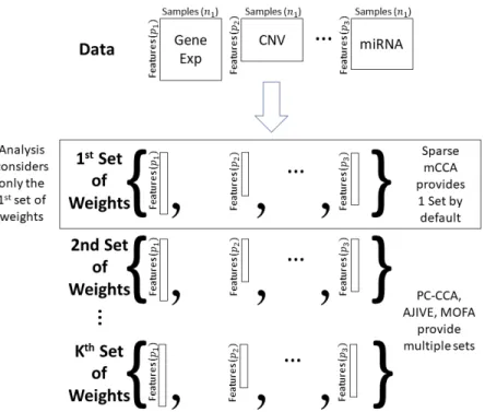
Each of the methods of interest provide sets of weights corresponding to the importance of each feature in each data type. The larger the absolute value of the weight, the more the corresponding feature contributes to the common variation. Instead of examining results in the feature space, we instead look on the sample space and observe relationships across data types and samples. This is accomplished by constructing what we call acontribution, which is calculated by multiplying the estimated weights and the data to obtain an individual contribution per subject. Letβˆibe thepi by 1 dimensional vector corresponding to the estimated weights for data typei, and letXibe thepibynmatrix corresponding to data typei. The contribution is then calculated asβˆi0Xi. Contributions can be calculated for any multi-omics method, as long as the output provides a list of weights. We will demonstrate how this is done in PC-CCA, Sparse mCCA, AJIVE, and MOFA. Because both PC-CCA and Sparse mCCA are modifications of Canonical Correlation Analysis (CCA), the calculation of the contributions are trivial. The weightsβiˆ in this case correspond to the solution for each data type, and a simple matrix multiplication can be performed to calculate the contributions. For AJIVE and MOFA, the contributions are not difficult to calculate; however, because these methods identify a multi-dimensional solution, we only focus on the weights for one factor (Figure 2.2). In AJIVE, this corresponds to the first column of the loadings matrix of the joint space, and for MOFA, this corresponds to the weights for the top factor. In the MOFA analysis, we restrict the method to fit only one factor.
Figure 2.2: Each method shown in the figure generates a set of weights for each data type. Our analysis only considers the first set of weights to avoid issues related to a potentially complex set of mappings of factors across data splits.
2.1.2 Cross-validation
The unsupervised nature of the multi-omic methods makes it difficult to determine whether a method is overfitting or identifying a true biological relationship. By omitting a subset of the samples from the analysis and predicting their contributions from each data type in the training set, we can discern whether the relationships from the full analysis suffer from overfitting or provide unstable results. Our analysis pipeline is shown in Figure 2.3. We chose to divide the data into training and test sets of approximately 80% / 20% of the total samples. Using the 80% training set, analyses were done for each method, and corresponding weights were generated for each data type. Contributions were calculated for the test set by multiplying the weights derived from the training set by the test set data in the manner appropriate to each method, as defined above. Critically, our cross-validation loop used for evaluation of methods takes placeoutsideof any permutation or cross-validation that a method may use during training or fitting of its model parameters, such as the calculation of feature weights for each data type.
different magnitudes. To account for this, we scale and change the sign of the cross-validated contributions to ensure that they are positively correlated with the results from the full analysis. This procedure is performed separately for each fold. The sign is flipped if the correlation between the cross-validated and full-analysis contributions is negative, while scaling is achieved by subtracting the mean and dividing it by either the standard deviation or the median absolute deviation. If the contributions are not unimodal or contain outliers, we recommend using the median absolute deviation for scaling.
To avoid difficulties in aligning weights across folds, in our evaluation we only consider the set of weights corresponding to the first factor. In MOFA, factors are arbitrarily labelled and thus no formal ordering is defined for the “first” or “second” factor. Repeating the analysis will yield a different labelling scheme for each factor while factors are still describing the same biological process. This necessitates the alignment of factors across multiple folds and creates a computational challenge. For sparse mCCA and MOFA, the first set of weights or first factor typically yields the strongest pair-wise correlations. As more sets of weights are estimated, the correlations typically decrease (see Fig 2b in (Argelaguet et al., 2018)). Lower factors may be more susceptible to fluctuations, such as sampling variability in the samples chosen for the training set.
After the contributions are appropriately scaled, contribution plots can be constructed for each pair-wise combination of the assays in the test set. We will refer to these plots as the cross-validation (CV) contribution plots and the contribution plots from the full analysis as the full contribution plots. By examining the change in correlations between the CV contribution plots and the full contribution plots for each pair-wise data type pair, we may observe the degree to which each method suffers from overfitting. The full contribution plots reflect the typical results that a user would observe when running a method on their entire dataset, while the CV contribution plots reveal any issues with thegeneralization of feature weights for new data, in that we observe the correlations obtained on all samples in the dataset
Figure 2.3: Pipeline for cross-validation analysis.Training Data: Dataset is subset to 80% of the original data and will be used to train the model.Multi-omics Methods: The training data are analyzed using the specified method.Output: Weights are output from the multi-omics methods.Test Data: The remaining 20% of the original data are used as test data and multiplied by the subsequent weights.Contributions: The result of multiplying the output weights by the test set data. Each sample in the test data yields one number that represents the contribution per data type.
2.1.3 Multi-omics Datasets
Data from The Cancer Genome Atlas (TCGA) (Wong et al., 2019) (The Cancer Genome Atlas Research Network et al., 2013) was used to evaluate method performance for Sparse mCCA, AJIVE, and MOFA. We applied these three methods to 558 breast cancer samples using Copy Number Variation (CNV), RNA expression, and micro RNA expression. CNV was summarized for 216 segments; RNA expression was measured for 12,434 genes; and miRNA expression was measured for 305 miRNAs. Five folds were selected for the analysis, and fold membership was fully randomized. Contribution and comparison plots were generated for each data type to evaluate the degree of overfitting and the consistency of the results.
Data from Li, et al (2016) was used as a second validation data set. This collection of datasets contained fewer samples and thus was used to examine stability of methods with smaller sample sizes. RNA expression, DNase, and protein expression were collected for lymphoblastoid cell lines from Yoruban individuals. DNase was measured for 699,906 peaks; RNA expression was measured for 13,967 genes; and protein expression was measured for 4,375 proteins for 53 samples.
2.2 Evaluation of Methods
We applied our evaluation framework to datasets with both large (TCGA breast cancer) and small (Li et al) sample sizes, as well as a permuted null dataset. Sparse mCCA, AJIVE, and MOFA all demonstrate consistency and a lack of overfitting in the large-sample size analysis. The overfitting plots for the large-sample size analysis (Figure 2.5 a-c) have near zero slopes, indicating that the relationships found in the training set generalize to the held-out set. The difference in the magnitude of the correlations across methods does not indicate a lack of overfitting, but rather that the top factor indicated a strong or weak relationship between the specified data types. This artifact is not necessarily a limitation of the method, but rather might be explained by the fact that we are considering only the first set of weights in our analysis. Side-by-side contribution plots (Supplementary Figures A.17 - A.25 ) also demonstrate a lack of overfitting and confirm that there are no sample outliers that are overly influencing the results. Comparison plots (Supplementary Figures A.26- A.28) show that the contributions for the CV analysis and full analysis are similar, indicating overall method consistency. AJIVE was observed to have reduced pair-wise correlations for contributions including the CNV assay, and this result persisted after attempting with a higher pre-specified rank (Supplementary Figure A.29). Overall, for the large-sample size analysis, we found that Sparse mCCA and MOFA did not overfit and found large pair-wise correlations between contributions from all assays. AJIVE also showed a lack of overfitting, however a large pair-wise correlation was only found between RNA and miRNA.
Alternatively, in the small-sample size analysis, Sparse mCCA and MOFA appear to overfit in the full analysis, while AJIVE does not overfit. Plot 2.5d shows a lack of overfitting with AJIVE in the small-sample analysis, while plots 2.5e and 2.5f show a consistent drop in the correlation for the CV analysis. Thus, sparse mCCA and MOFA are able to identify strong linear relationships in the full analysis, but the correlations are substantially reduced in the CV analysis. This may reflect a reduced ability for consistent detection of top factors for small-sample datasets. Side-by-side contribution plots (Supplementary Figures A.34 - A.42) show more clearly a decrease in correlation with Sparse mCCA and MOFA, but not with AJIVE, which maintains a relatively weak correlation in both analyses. Comparison plots (Supplementary Figures A.43 - A.45) show less consistency than in the large-sample analysis.
We assessed the degree to which the results were robust when varying the number of folds. Sparse mCCA was used to analyze the small-sample size dataset using both 3 and 10 folds. The 3 fold analysis yielded small training set sizes, which led to poor prediction for the test set samples (Supplementary Figure A.46). Alternatively, in the 10 fold analysis, small test set sizes made contribution scaling difficult, which also led to reduced correlation of the cross-validated contributions with the full set contributions (Supplementary Figure A.47). Additionally, many methods have extensive run times and thus conducting an analysis with many folds can create a prohibitive computational burden.
Figure 2.6: Side-By-Side contribution plots fora)PC-CCA with 100 PCs andb)Sparse mCCA with the null dataset: Left panels show the contribution plots from the full analysis, while right panels show the contribution plots for the CV analysis. Pair-wise correlations are reported on the figure.
2.3 Discussion
There are now dozens of methods for unsupervised multi-omics data analysis, and the list continues to grow. Other multi-omics approaches that we did not compare here use re-formulations of partial least squares (PLS) (Lˆe Cao et al., 2009) , or co-inertia analysis (CIA) (Meng et al., 2014), and often make use of lasso penalty or sparse thresholding to induce sparsity on feature weights.(Rohart et al., 2017)
Future work may include investigation into the alignment of weights across folds and replications and how to incorporate more than one set of weights. Argelaguet et al (2019) (Argelaguet et al., 2019) propose comparing the Pearson correlation coefficient between every pair of factors as a way to address these concerns. Additionally, classical CCA could be used to perform matching of factors across folds or replicate runs, by running CCA on every pair of contributions. We did not evaluate the sensitivity and specificity of the methods we tested, as they are designed to describe variation, rather than classification, of samples. A separate analysis similar to Pucher et al (2018) (Pucher et al., 2019) would be needed to evaluate AJIVE and MOFA on the claims of accuracy. Here we examined the biological meaningfulness of the top factor found in the TCGA breast cancer dataset by plotting the mRNA contributions against expression of estrogen receptor 1, for which we have from literature some external support of its relevance as a primary axis of co-variation of molecular profiles of breast tumors. In general, downstream assessment of the biological meaningfulness of a factor can be achieved through gene set analysis, by defining the observed gene set as the non-zero or top weighted genes from the gene expression weights estimated by the multi-omics methods. The MOFA R package includes a function for performing this type of “Feature Set Enrichment Analysis”. For non-gene expression features, non-zero or top weights for features can be examined with respect to their co-localization with weights from other data types on the genome, or with various publicly available genomic tracks such as cell-type specific regulatory regions (ENCODE Project Consortium, 2012)(Roadmap Epigenomics Consortium, 2015).
CHAPTER 3: ACTOR - A LATENT DIRICHLET MODEL TO COMPARE EXPRESSED ISO-FORM PROPORTIONS TO A REFERENCE PANEL
The relative proportion of RNA isoforms expressed for a given gene has been associated with disease states in cancer, retinal diseases, and neurological disorders. At the gene level, expression can be functionally characterized by known gene sets. However, there is less annotation data at the transcript level and there are fewer statistical methods designed specifically for recognizing characteristic splicing patterns. An alternative approach would be to characterize the splicing patterns in a sample, or set of samples, by comparing the patterns to those seen in a large reference panel. While some methodological comparisons have been made in the area of clustering samples based on isoform splicing, less development has been made in comparing experimental data to a reference panel. Leveraging large public datasets produced by genomic consortia as a reference, one can compare splicing patterns in a dataset of interest with those of a reference panel in which samples are divided into distinct groups (tissue of origin, disease status, etc.). We propose ACTOR,Alatent Dirichlet model toCompare expressed isoform proportionsTOaReference panel, to relate isoform splicing patterns in an experimental dataset to an independent reference panel composed of discrete sample groupings. We provide gene level interpretations of the relatedness across experimental samples and provide an improvement to standard distance-based approaches. ACTOR was validated using data from the Genotype-Tissue Expression project (GTEx) and accurately identified genes and gene classes for which isoform splicing was similar across tissues.
3.1 ACTOR
reference group combinations, which reduces the reference panel to a more manageable size. For a sample (j) in the experimental dataset, we calculate a per gene (g) likelihood conditional on the parameter estimates coming from a specific reference panel group (s) asp(Xgj|αgs). Using these likelihoods, we
wish to identify latent groupings of genes that are spliced in a similar manner to our reference groups. Identifying these gene classes can be a challenging task, and topic modeling through the use of Latent Dirichlet Allocation (LDA) can provide a means to accomplishing this task. Figure 3.7 provides a visualization of our method and Supplementary Table B.5 provides a table of all notation for this model.
Figure 3.7: ACTOR uses precomputed Dirichlet parameters for each reference group to identify which reference group a set of experimental samples is most similar to based on isoform splicing patterns. The curves represent the Dirichlet distribution for each reference group. ‘X’ corresponds to an experimental sample. For visual simplicity, a one-dimensional simplex is shown here.
Additionally, we add a second latent component to identify sets of genes, which we call gene classes, that have similar reference group distributions. Dirichlet Multinomial estimates for each reference group in our reference panel are pre-calculated, so while the reference group assigned to a gene in our experimental dataset is a latent variable, the groups themselves are not latent, nor are the parameters describing the distribution of isoform proportions for a given group. In contrast, the topics in the text-mining LDA formulation are latent, and discovered during model fitting, while the gene classes are latent in our model. This reference group assignment within the LDA model makes use of the likelihood conditional on the reference group estimates.
As mentioned earlier, it is also informative to identify classes of genes that align to the groups in the reference panel similarly. A sample could splice similarly to the reference groups across one collection of genes, while splicing similarly to a different set of reference groups in another collection of genes. The splicing could also be characterized as being unique to one reference group or as a mixture across multiple groups. We will use the term “gene class” to indicate a collection of genes in the experimental samples that have a similar relation to the reference groups. All genes within the same class have a common probability vector corresponding to the reference group from which they are generated. Supplementary Figure B.50 gives a toy example, with five reference panel groups and four gene classes. Three of the gene classes correspond to sets of genes that are all spliced similarly to one specific reference group. Gene class 1 aligns with reference group 1, gene class 2 aligns with reference group 2, and gene class 4 aligns with reference group 5. We also see that there could be situations in which genes are spliced similarly to two different reference groups. Gene class 3 is shown to be equally similar to reference groups 3 and 4. Therefore, we aim to estimate both reference group and gene class membership using a generative probabilistic model in a manner similar to LDA. The user prespecifies the number of gene classes the model will try to fit. As will be seen in the results, an overestimate of the number of classes will result in the model creating empty gene classes for those that are not needed.
opposed to only one set of relevant samples. In addition, the reference panel in our setting has known group structure (e.g. samples belonging to tissues). (Dey et al., 2017) also looked at identifying RNA-seq structure using latent memberships, however this is also distinct from our approach as they model the counts as coming from a Multinomial distribution with a different proportion parameter per sample rather than utilizing a Dirichlet distribution to model the extra variability.
Figure 3.8: Graphical model representation of our proposed framework. Figurea)corresponds to the full model while Figureb)corresponds to the variational distribution.
ACTOR is a hierarchical latent class model with the first level of latent classes being informed by the reference panel. The first step of the generative model is to generate a probability vector (γ) of length C(number of gene classes) for the gene class assignment from a Dirichlet distribution with unknown parameterωof lengthC. This probability vector is common for all genes. For each gene class (l), a probability vector of lengthT (number of reference groups) is drawn for the reference group assignment (θl) from a Dirichlet distribution with unknown parameterβ. βis of lengthT and is common for all
gene classes. For each gene, a gene class (cg) is drawn from a Multinomial distribution with parameter
γ, which was generated in the first step. Then for each gene, a reference group (tg) is drawn from
the Multinomial distribution using the reference group probability vectorθlthat corresponds with the
selected gene class (cg). In the formulation below,Θ= (θ1, ...,θC)0is aT xCmatrix andcgis a vector