Optimization of an Injection Locked Laser System for Cold Neutral Atom Traps

(1)

Optimization of an Injection Locked Laser System for Cold Neutral

Atom Traps

A Senior Project

presented to

the Faculty of the Physics Department

California Polytechnic State University, San Luis Obispo

In Partial Fulfillment

of the Requirements for the Degree

Bachelor of Science

by

Elliot Lehman

March, 2019

c

(2)

Abstract

(3)

List of Figures

1 Intensity distribution pattern from a 780nm laser incident upon a pinhole of radius

50µm [1]. . . 4

2 Seed laser configuration. . . 5

3 Injection locking setup. Figure adapted from Figure 13 of Alex Crawford’s Senior Project [2]. . . 6

4 Photograph of injection locking setup. The numbers labelled on the photograph correspond to the numbered list of optical components. . . 7

5 Basic GPIB control and communication sequence. . . 9

6 Labview front panel. . . 11

7 Receiving laser natural wavelength (nm) distribution with counts on the y-axis. . . . 12

8 Injection locked wavelength distribution. . . 13

9 Pulling effect wavelength distribution. . . 13

10 Pushing effect wavelength distribution. . . 14

11 Depletion effect wavelength distribution. . . 14

(5)

1 Introduction

1.1 Quantum Computing

Classical computers utilize digital signals and logical gates, most often made from transistors, to perform computations. Features in modern processors continue to be manufactured at smaller scales, since smaller feature size often yields faster and more efficient performance. As these features become smaller, quantum effects become increasingly more problematic [3]. Quantum computers, however, are built specifically to use quantum effects to perform computations.

Some algorithms used by quantum computers have been shown to be far more efficient at providing solutions to certain problems when compared to a classical computer. For example, only a quantum computer can efficiently simulate true quantum systems. Using Shor’s algorithm, quantum computers would be able to solve prime factorization problems, widely used in encryption worldwide [4]. By nature of quantum information, ultra-secure communication channels could also be produced [5].

1.1.1 Qubits

The most fundamental piece of information in a classical computer is the bit. For a quantum computer, the bit’s analog is a ”qubit.” A classical bit is binary and discrete. It exists in one of two states, the 1 state or the 0 state. A qubit also has two observable states, but exists as a superposition of each observable state. The state of a single qubit can be represented as:

|Ψsinglei=α|0i+β|1i (1)

The states |0i and |1i are the two observable states. The coefficients α andβ are the probability amplitudes of the respective states being observed. They must satisfy the normalization condition:

|α|2+|β|2= 1 (2)

This can be generalized to a function that describes a multi-qubit system. A two qubit system can be represented as:

|Ψ2−qubiti=α|00i+β|01i+γ|10i+δ|11i (3)

Similarly to classical computers, quantum computers also need gates. Just as the NAND gate is a universal gate for bit operations [6], universality can be achieved in a quantum computer by combining single qubit gates and an entangling gate [7]. This makes entanglement a key aspect of a quantum computers functionality.

1.1.2 Quantum Computer Necessities

Since quantum mechanics dictates the behavior of an enormous range of physical systems, there exist many approaches to physically realizing qubits and quantum gates. In general, there are five requirements, listed below, that govern the creation of a quantum computer [8]. A system of neutral atoms (Rubidium-87 atoms in our case) in an optical lattice is a good candidate to achieve these goals.

1. A scalable physical system with well characterized qubits

(6)

2. The ability to initialize the state of the qubits to a known state

This is a requirement for any computer. Without knowing the initial states of the system, the processes done on the system will produce meaningless results. Initialization can be achieved in our system by exposing the atoms to light with frequency equal to the an excitation frequency for a single ground state.

3. Long relevant coherence times, much longer than the gate operation time

Coherence time describes how long the qubits are stable for. If the coherence times are shorter than it takes to perform an operation, the operation will fail or produce meaningless results. Neutral atoms are a good choice for this because their weak atomic interactions make it possible to trap a large number of atoms in close proximity at once.

4. A “universal” set of quantum gates

As stated previously, to create a set of universal quantum gates, a single entangling gate combined with single qubit gate can be used. Entanglement can be achieved with Rb-87 atoms by introducing atomic dipole-dipole coupling [9, 10, 11].

5. A qubit-specific measurement capability

The result of the computation must be able to be read. This is achievable with atoms using spectroscopy to determine the energy state of the atoms.

2 Theory

In order to use Rb-87 atoms as qubits, they must be confined to a specified region of space so that single and pairs of qubits can be individually addressed. In order to do this, a large group of atoms is cooled and confined to a region of space using a magneto-optical trap (MOT). Once confined to this region, the MOT is quickly switched off and the optical trap is turned on, isolating atoms in desired regions of space.

The optical trap is a dipole trap composed of a laser, detuned from atomic resonance, that shines through a pinhole which creates a diffraction pattern. Depending on the detuning of the laser, the atom is then confined to either the area of highest or lowest intensity of the diffraction pattern. The strength and effectiveness of these traps is governed by the laser intensity and the detuning of the laser. An injection-locked laser is used to provide maximum intensity while still providing the ability to precisely tune the output frequency. Being able to precisely tune the output is critical to use to atoms for quantum computing, since unwanted atomic absorption of photons would destroy the computations.

2.1 Trapping Atoms with Diffraction Patterns

2.1.1 Atomic Dipole Traps

When an electromagnetic wave is incident upon an atom, it induces an atomic dipole. The induced dipole then interacts with the wave. The relationship between dipole moment and potential energy is

U =−~p·E.~ (4)

As the light’s frequency nears one of the atom’s resonant frequencies, the induced dipole moment’s magnitude increases. The relationship between dipole moment strength and detuning is

~

(7)

with

α= e

2

me

1

ω2

o−ω2−iωΓω

. (6)

where ω is the angular frequency of the light, ωo is the resonant angular frequency, e is electron

charge,meis electron mass, and Γωis the radiative decay rate of an electron oscillating at an angular

frequencyω [12]. The dipole potential energy can be expressed as

U(r) =β~Γ

8 Γ ∆

|E(r)|2 |Es|2

(7)

whereβ is the line-strength factor, Γ is the spontaneous decay rate,Esis the saturation field of the

transition, and ∆ is the laser detuning [1]:

∆ =ω−ωo (8)

If the laser is tuned to be higher than resonant frequency, then the it is called blue-detuned (BDT). BDT traps confine atoms in regions of low intensity. If lower than resonance, then it is called red-detuned (RDT). These confine atoms to regions of high intensity. Equation (7) suggests that small detuning would be desirable in order to create a strong trap. However, the probability of the photon being absorbed by the atom increases as detuning gets smaller [13]. The power from photons absorbed by the atom is

Pabs=

ω 0c

Im(α)I (9)

whereI is the field intensity [14].

Since it is undesirable to disturb the atom’s energy state with the trap laser, it is important that the laser is detuned to minimize scattering. Because the trap depth is proportional to the intensity, a strong trap with a minimal scattering rate can be produced by increasing both detuning and intensity. The requirement for a higher intensity is why the injection locking laser amplification is needed.

For an atom to be trapped, stationary areas of either high or low intensity need to be produced. Many diffraction patterns produce intensity distributions like this. This experiment utilizes a pinhole diffraction pattern as it is relatively easy to manufacture and can also make both RDT and BDT traps [15].

2.1.2 Pinhole Diffraction

The diffraction pattern chosen for this experiment is a pinhole diffraction pattern. As shown in the figure below, there exist well defined bright (high intensity) and dark spots (minimal intensity) in the pattern. Since the pattern is radially symmetric, these light and dark regions are able to confine the atom three-dimensionally.

For this experiment, the most appropriate description of the electric field produced by the pinhole diffraction is produced using the Rayleigh-Sommerfeld regime. For a laser, approximated as a plane wave, incident on a circular aperture atz= 0, diffraction along the +z axis can be modeled by the following equation [12].

Sz(0,0, z) =S0

1 + 2(z_a)2

1 + (z a)

2 −

2z_a

p

1 + (z_a)2 ×cos

kz

r

1 + (a

z)

2₋₁

!

(10)

The intensity of light incident upon the aperture isS0,ais the radius of the aperture, and k

(8)

Figure 1: Intensity distribution pattern from a 780nm laser incident upon a pinhole of radius 50µm [1].

2.2 Laser Injection Locking

2.2.1 Laser Basics

The purpose of a laser is to produce light that is spatially and temporally coherent by ampli-fying a desired wavelength of light. There are three basic elements that make a laser: the medium, the pump, and the resonator.

There exists a wide range of media that can be used to create a laser. In this experiment, a semiconductor (GaAlAs) is used as the medium for the lasers. The medium of the laser is what absorbs the pump’s energy and emits light. The laser pump refers to the energy source of the laser. The pump excites atoms in the medium to a state just above the lasing energy, from which it rapidly decays to a metastable state. This state is known as the “upper laser level.” It is from this state that the atoms decay to the “lower lasing level.” The photons produced in this transition are the ones that will be reflected and amplified within the resonator. A resonator consists of two mirrors, one totally reflecting and one semi transparent, which allows the laser to output light. The light that reflects between the mirrors stimulates transitions from the metastable state to the lower laser level, resulting in the amplification of photons resonant with that transition [16]. In semiconductor lasers, conduction and valence bands take place of the atomic states, and the photons are reflected by the polished facets of crystal.

2.2.2 Injection Locking

Laser injection locking is an effect that utilizes a “seed” laser to make the “receiving” laser generate a desired wavelength of light. Injection locking occurs when light from the seed laser is injected into the receiving laser, stimulating emission of photons coherent with the injected photons, thus causing the receiving laser to emit light of the same wavelength as the seed laser.

Injecting light into the receiving laser using the seed laser does not guarantee injection locking will occur. If the seed laser wavelength,λS, is far enough away from the wavelength of the receiving

laser, λR, the effect on the receiving laser is negligible. WhenλS is within a range of λR, effects

(9)

region differs from the “lock zone” in that the locking region only refers to the range of wavelengths at which the lock occurs, whereas the lock zone refers to the entire parameter set that determines the coupling between the lasers. These parameters include, but are not limited to, each laser’s driving current, each laser’s temperature, and the optical power injected into the receiving laser.

The effects of injecting light into the receiving laser are not limited to locking. One common effect is when the seed laser can be observed to be “pulling” asλRshifts nearerλS, but does not lock

entirely. This often occurs as eitherλR orλS is tuned to be nearer the other. A less common, and

perhaps more interesting effect is when the seed laser can be observed to be “pushing” the receiving laser, as the receiving laser spectra has two distinct peaks, one beingλS, and the other being further

away from the initialλR.

For this experiment, injection locking is used to amplify the seed laser wavelength to produce enough light to trap Rubidium atoms within the pinhole diffraction pattern.

2.2.3 Seed Laser Configuration

To control the seed laser wavelength, a laser grating feedback configuration, known as a Littrow configuration, is used. This configuration, shown below, consists of a diffraction grating placed directly after the laser diode. The diffraction grating is movable and controllable via a piezoelectric transducer (PZT). By changing the angle of the diffraction grating, different laser modes are selected to be reflected back into the laser. This mode is amplified by the laser and becomes the dominant mode. Since the selected mode is reflected back into the diode, this laser is an external cavity laser diode.

Figure 2: Seed laser configuration.

All tests in this experiment were done using a single, fixed wavelength of the seed laser. However, this system will be controlled and stabilized electronically. This system allows for fast and precise control of laser output, but it does sacrifice approximately 40% output power. Thus, injection locking is needed to amplify the output.

3 Experiment

3.1 Injection Locked Laser Setup

(10)

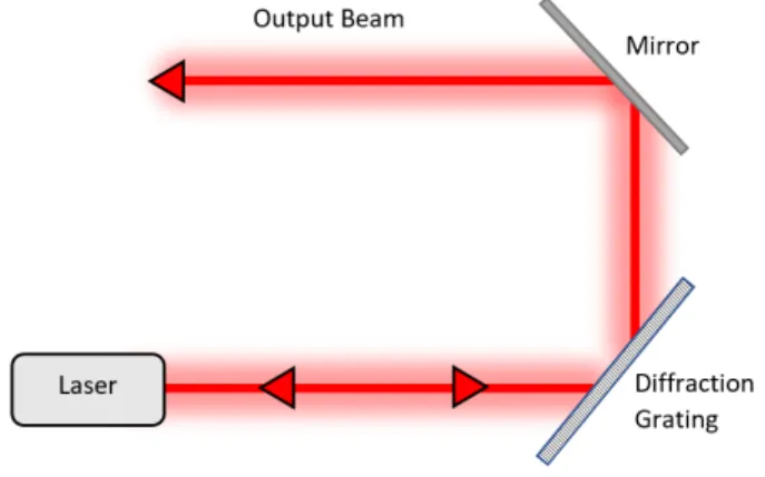
Figure 3: Injection locking setup. Figure adapted from Figure 13 of Alex Crawford’s Senior Project [2].

To set the system up, as pictured in Figure 4, the following optical components are needed: 1. Faraday Isolator (FI)

A faraday isolator is used to prevent back reflections transmitting into the L1 cavity. 2. Half-Wave Plate (HWP)

Half-wave plates introduce a πphase shift along the slow axis of the plate. This rotates the linearly polarized light to a desired direction with minimal intensity loss.

3. Mirror (M)

Mirrors are used to direct the beam along the desired path. 4. Polarizing Beam-Splitter Cube (PBSC)

Polarizing beam-splitter cubes allow one direction of polarized light to be transmitted while reflecting light with polarization orthogonal to the transmitted light. In this system, it is used to direct the seed laser light into the receiving laser while allowing the receiver output to be transmitted out of the system.

5. Faraday Rotator (FR)

The Faraday rotator rotates the beam 45o clockwise regardless of the direction of beam prop-agation. This orients the incoming seed beam so that the polarization matches that of the receiver beam. It also rotates the receiver beam polarization the additional 45o needed to for the beam to be transmitted through the PBSC.

6. Iris (I)

Irises are used to improve the alignment of the system.

(11)

laser and positioned it at an angle such that the power through the polarizer from the receiving laser was maximized. Then, leaving the polarizer set to that angle, I rotated the receiving laser HWP such that the power through the polarizer from the seed laser was maximized. This process ensured that the seed light entering the receiver cavity was the same polarization as the natural polarization of the receiver. This process also ensured that the receiver laser light transmitted through the PBSC was maximized.

Figure 4: Photograph of injection locking setup. The numbers labelled on the photograph correspond to the numbered list of optical components.

3.1.1 Collimation of Receiving Laser

It is important that both lasers are collimated so that their rays are parallel throughout the entire experiment. Using the spanner wrench, the focus of the laser can be adjusted. Different screwdrivers or wrenches may be used, but the spanner wrench designed for this makes the job slightly easier since it has an opening that allows the beam to pass through. To collimate the laser, the focus needs to be brought to infinity. In practice, this means that the beam must not have a focus within a distance much greater than the distance the beam will travel to the trap.

(12)

the beam is brought up to that height. This minimizes the use of unsecured mirrors, making the collimation setup significantly more robust.

In the beginning, the location of the beam’s focus may be unknown and difficult to find. If this is the case, it is useful to bring the focus close to the laser and work from there. Once the focus of the laser was known, I slowly brought the focus further away from the lens, until the beam was uniform throughout the collimation path.

3.1.2 Alignment of the System

Alignment of the system is critical to its functionality. Since the seed laser’s photons need to resonate within the receiver cavity, the seed beam needs to enter the receiving laser at the same angle that the receiver beam leaves. This was achieved by overlapping the beams using irises. To overlap the beams, only the beam path of the seed laser was altered using the kinematic mounts holding the mirror and PBSC.

To align the system using irises, I placed one iris directly in front of the receiver output and one as near as possible to the PBSC. The further the irises are from each other, the smaller the angular deviation of the beam that is allowed. First, the irises were closed so that the aperture size was minimized. This also improves the alignment. Then, the seed beam was moved using the kinematic mounts to also go through the two irises. A Thorlabs power meter was used to maximize the power through both irises, ensuring the best possible alignment.

3.1.3 Laser Diode Temperature Stabilization

Since the temperature of the laser diodes affects what frequencies of light they produce, and affects the locking efficiency, it was important that their temperatures were stable throughout the measurement period. The temperatures of the lasers are controlled using the Thorlabs ITC502. This controller allows the user to choose a desired thermistor set point. The controller then drives the thermoelectric cooler with a current defined by the PID settings. These settings determine what response the controller has to the difference in set and actual thermistor resistance.

The PID settings can be controlled using the knobs on the front panel of the machine or by sending commands using GPIB. The optimal PID settings are the ones that force the temperature of the laser to reach the set temperature in the shortest amount of time with the least amount of fluctuations. Since each laser has slightly different thermal properties due to differences in construc-tion, each laser will have different PID settings. The general procedure is to change each variable (P, I, or D) independently and plot temperature against time. The parameters are changed until suitable settings are found. Two key features can be used to identify suitable PID settings: short initial time to reach set temperature and only small, damped oscillations after the set temperature is reached.

This process was done manually, but the automation program described below can be easily modified to automate a search for optimal PID parameters. Automating this search could accelerate the process of PID tuning from multiple hours to minutes in the lab.

3.2 Injection Locking Efficiency Measurement and Automation

3.2.1 Determining Injection Locking Efficiency

Injection locking efficiency is determined by measuring the output spectrum of the receiving laser. It is calculated as the ratio of the intensity at the dominant seed laser wavelength to the sum of the intensities of the receiver output, which is approximated as the sum of the intensities at the seed wavelength and the initial dominant receiver wavelength:

e_IL = IS

IS+IR

(13)

Although the coupling between the seed and receiving laser is more complicated than the relationship between two laser modes,eIL still provides a good measure for the effectiveness of this

laser amplification system since a high value indicates that the receiving laser is lasing at the seed laser wavelength.

The intensity of each wavelength is measured by measuring photon counts over a specified amount of time using the Ocean Optics spectrometer. The Ocean Optics OOIBase32 software can display a live plot of the current spectrum, which is useful for tuning the laser system in real time. The software can also be configured for data taking over time. Up to six wavelengths can be selected to write to a single file, which contains their respective counts during each acquisition time. This mode streamlines the process for taking data over longer periods of time, because the output file format requires less processing. The procedure for using the spectrometer in this mode is covered in Alex Crawford’s Senior Project (p. 25) [2].

If data on more than six wavelengths is needed, data for the entire spectrum can be saved for each acquisition by checking the box in theConfigure Acquisition tab. The downside to this mode is that the files are larger and require slightly more processing to extract the relevant information.

After obtaining preliminary results showing that injection locking was occurring at some laser settings, it became clear that there was a wide range of laser settings at which injection locking was either not occurring or its effects were negligible. Since the relationship between injection locking efficiency and each laser control parameter appeared to be nonlinear, it was difficult to predict what settings should be used. Therefore, it was necessary to automate a search for lock zones.

3.2.2 Automation of Data-Taking Using LabVIEW

To automate the parameter search, I created a LabVIEW VI. LabVIEW is an ideal program for this since both interfacing with GPIB instruments and creating a GUI are straightforward. Our GPIB lab instruments are connected to the lab computer using the Agilent 82357B USB/GPIB Interface. If only single commands need to be sent, the most straightforward way to do this is using the Agilent GPIB to USB software. This is especially useful for troubleshooting.

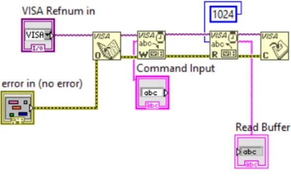
Figure 5: Basic GPIB control and communication sequence.

(14)

VI. This VI has a string input that controls what string is sent to the GPIB device. The ”VISA Out” terminal is then wired to the ”VISA Read”, which has a string output to receive strings from the instrument. Finally, the ”VISA Out” from this VI is wired to the“VISA Close” VI, which then closes the communication channel. Once this series of VIs are connected, the user can send commands and receive data by executing the program. This sequence is shown above.

To streamline the process further, I used the above series of VIs to create the following Sub-VIs to communicate with the ITC502:

Send and Receive

– This VI consolidates the four VIs discussed above into a single VI that can be used to send any command to the instrument and receive its response. This Sub-VI is a building block that can be used to create other VIs for commands and responses not yet created.

Terminals:

∗ VISA Resource Name: Wire the GPIB address of the desired instrument to this terminal.

∗ String In: Wire a string with the command you want to send.

∗ String Out: This receives data from the instrument. To write receiving data to a file, ”Write to Delimited File” can be used

Send Command

– This VI is used to send commands when a response is not needed. Terminals:

∗ String In: Wire a string with the command you want to send.

Read Temp

– This VI reads laser diode temperature. Terminals:

∗ String Out: This outputs a string with the current TEC thermistor reading.

Read Current

– This VI reads laser diode current. Terminals:

∗ String Out: This outputs a string with the laser diode current reading.

(15)

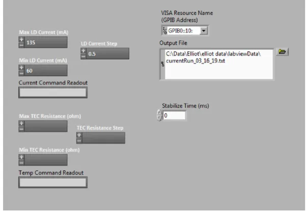
Figure 6: Labview front panel. Values that need to be input are:

Max LD Current:

– The maximum laser diode current value in (mA) for the sweep. If the value sent to the ITC502 is above the set current limit, the command will not be executed. It is uncommon for the lasers to be set above 135 mA.

Min LD Current:

– The minimum laser diode current value in (mA) for the sweep.

LD Current Step:

– Defines laser diode current step size in mA.

Max TEC Resistance:

– The maximum TEC thermistor resistance for the sweep. If the value sent to the ITC502 is outside the set thermistor window, the command will fail.

Min TEC Resistance:

– The minimum TEC thermistor resistance for the sweep. If the value sent to the ITC502 is outside the set thermistor window, the command will fail.

TEC Resistance Step:

(16)

Stabilize Time:

– This sets the time for the ITC502 to stay on each setting in the sweep. This is necessary because the laser diode temperature needs time to stabilize after a current or thermistor value change and the response of the receiving laser takes time to stabilize as well. A typical value when only varying current is 3 minutes. For smaller steps, it may be possible to set this time shorter. For large temperature changes, this time should probably be increased.

Output File:

– Put the file path here for the VI to write data to. Specify this before running the program. 3.2.3 Identifying Lock Zones

There are two ways to identify lock zones: mathematically and visually. Mathematically, lock zones are identified by having a largeeIL value. Although this may be a more precise way to

define lock zones, it is not always feasible to measure an accurate eIL value while changing laser

parameters, since changing laser settings results in changes of laser wavelengths. This means that each time a parameter is changed, it is necessary to remeasure the seed and receiver wavelengths so thatIS andIR can be measured accurately. Currently, when the seed laser wavelength needs to be

measured, an additional beam splitter is placed in the path of the seed laser and the spectrometer fiber is moved so that the split beam is incident upon the fiber. This means that measuring the seed laser wavelength and the receiver wavelength was not practical to automate during the time of this project. Instead of creating a system to automate this process, I identified many lock zones visually by viewing plots of the spectrometer data.

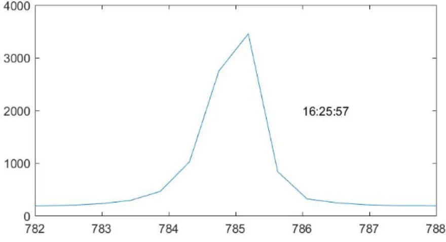
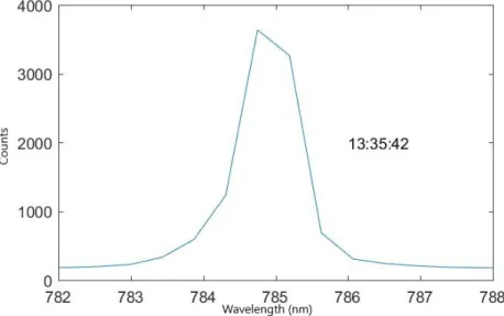
The main characteristic of a spectrometer plot that identifies a lock zone is a peak at the seed wavelength. If the system is well-aligned, the spectrometer should record almost no counts due to reflections from the seed beam. If a peak is seen near the seed wavelength channel, then this is evidence of a lock zone. In general, there are four different coupling behaviors that indicate a lock zone that can be seen when viewing the spectrometer plots. Descriptions and figures are below. All plots are timestamped to allow for easier time correlation.

For reference, the first figure shows the wavelength distribution with negligible coupling.

(17)

Figure 8: Injection locked wavelength distribution.

The second effect is the “pulling” effect. This effect can be identified by a shift in the dominant wavelength towards the seed wavelength.

Figure 9: Pulling effect wavelength distribution.

(18)

Figure 10: Pushing effect wavelength distribution.

One of the most common effects is depletion of counts at the dominant wavelength.

Figure 11: Depletion effect wavelength distribution.

(19)

Figure 12: Double peak wavelength distribution.

Since a single overnight data-taking run can produce thousands of these images, a convenient way to view them is by producing a video where each image is a frame. I used MATLAB to produce the plots and create videos from the frames. There are also many standalone programs that could be used to easily produce videos this way.

3.2.4 Lock Zones

With the receiving laser at a set temperature of 14.5 kΩ and a set current of 134.95 mA, I varied the seed laser current from 50 mA to 135 mA in steps of 0.5 mA for four temperatures: 14.0 kΩ, 14.2 kΩ, 14.3 kΩ, and 14.4 kΩ. Few zones with full locking were found, but many areas of strong coupling were discovered.

For 14.0 kΩ, no coupling was observed until the seed current reached 116.4 mA. This was the highest required current to observe coupling out of the four temperatures studied. Splitting was observed at 118.0 mA and beyond, and pulling was observed at 129.2 mA. For 14.2 kΩ, weak splitting was observed at 64.7 mA, and strong splitting and pushing effects were observed from 109.0 mA onward.

Stronger coupling was observed for 14.3 kΩ. Splitting was observed starting at 69.7 mA, a significantly lower coupling current than the previous two temperature settings. A complete lock was produced at 89.7 mA, but was not produced immediately before or after this current. Strong pulling effects and stable splitting effects were observed after 109.5 mA.

The final temperature tested, 14.4 kΩ had the lowest coupling current of 64.7 mA. Weak splitting was observed starting at 64.7 mA and strong splitting and pushing was observed starting at 109.0 mA.

(20)

4 Conclusions

4.1 Results

Using the LabVIEW program and MATLAB-produced videos, I obtained preliminary results for laser settings that can be explored further. The rarity of the lock zones within the parameter ranges tested shows the need for automation for finding effective laser settings for injection locking. The results showed seed laser temperatures nearer the receiver laser temperature produced the strongest coupling effects. The results also show that the minimum current needed to observe coupling is dependent on the temperature of the seed laser, and they show that coupling does not necessarily increase with an increase in current. The most promising seed laser settings were: a temperature of 14.3 kΩ with a current of 89.7 mA, and a temperature of 14.4 kΩ with a current between 109 mA and 135 mA. The 14.3 kΩ sweep produced the most definitive lock, but the 14.4 kΩ sweep produced more coupling throughout a wider range of currents. Both temperatures should be studied further with more precision, and currents near 89.7 mA should be studied while varying temperature in much smaller step sizes.

4.2 Future Work

Lock zones varied in size, meaning that for some lock zones, small changes in any variable (laser diode current or temperature, and optical power input) could cause the lock to be lost. This means that it is possible that there were small lock zones that were completely missed by the initial parameter sweeps due to their relatively large step sizes. The same type of search with more precise step sizes may yield new results.

(21)

5 References

[1] Gillen-Christandl, Katharina, and Glen D. Gillen, “Projection of Diffraction Patterns for use in Cold-Neutral-Atom Trapping,”Physical Review A82.6 (2010): 063420.

[2] Crawford, Alex, “Assembling and Characterizing the Efficiency of an Injection Locked Laser System for Cold Neutral Atom Optical Traps,”Cal Poly Senior Project, 2018.

[3] Sperling, Ed, “Quantum Effects At 7/5nm And Beyond,”Semiconductor Engineering, 2018. [4] Neilson, Michael A. and Isaac L. Chang, Quantum Computation and Quantum Information.

Cambridge University Press, 10th anniversary ed., 2010.

[5] Wang, Chuan, Fu-Guo Deng, Yan-Song Li, Xiao-Shu Liu, and Gui Lu Long, “Quantum secure direct communication with high-dimension quantum superdense coding,”Physical Review A71 (2005): 044305.

[6] Galvez, Enrique J.,Electronics with Discrete Components. John Wiley & Sons, 2013.

[7] Lloyd, Seth, “Almost Any Quantum Logic Gate is Universal,” Physical Review Letters 75.2, 346 (1995).

[8] DiVincenzo, David P., “The Physical Implementation of Quantum Computation,” arXiv preprint quant-ph/0002077, 2008.

[9] Deutsch, Ivan H., Gavin K. Brennan, and Poul S. Jessen, “Quantum computing with neutral atoms in an optical lattice,”arXiv preprint quant-ph/0003022, 2000.

[10] Isenhower, L.et al, “Demonstration of a Neutral Atom Controlled-NOT Quantum Gate,” Phys-ical Review Letters 104, 010503 (2010).

[11] Wilk, T. et al, “Entanglement of Two Individual Neutral Atoms Using Rydberg Blockade,”

Physical Review Letters 104, 010502 (2010).

[12] Gillen, Glen D., Katharina Gillen, Shekhar Guha, Light Propagation in Linear Optical Media. CRC Press, 2014.

[13] Liboff, Richard L.,Introductory Quantum Mechanics. Addison-Wesley, 4th ed., 2002.

[14] y. Grimm, R. and Weidem¨uller, journal = arXiv:physics/9902072, “Optical dipole traps for neutral atoms,”

[15] Gillen-Christandl, Katharina, and Bert D. Copsey, “Polarization-Dependent Atomic Dipole Traps Behind a Circular Aperture for Neutral-Atom Quantum Computing,”Physical Review A

83.2 (2011): 023408.

[16] Pedrotti, Frank L., Leno M. Pedrotti, Leno S. Pedrotti, Introduction to Optics. Cambridge University Press, 2006.

[17] Kavanaugh N.et al, “Stable injection locking with slotted fabry–perot lasers at 2µm,”J. Phys. Photonics 1 (2019) 015005.

(22)

6 Appendix

MATLAB Script

% Elliot Lehman %

% Matlab script to plot ocean optics spectrometer data and create a video using % each capture.

% % 2019

% Creating string arrays needed to import scope files. num_files = 1077;

for n = 1:num_files

file_index{n} = num2str(n-1); for i = 1:5

if length(file_index{1,n})<5

file_index{1,n} = strcat(’0’,file_index{1,n}); end

end end

% Extracts only the scope files of interest; n can be any integer range between 0 % and num_files.

for n = 300:num_files

scopeFile = strcat(’specRun_03_04_19.txt.’,file_index{1,n},’.Master.Scope’); delimiterIn = ’\t’;

headerlinesIn = 19;

A = importdata(scopeFile, delimiterIn, headerlinesIn);

% We’re not interested in the entire spectrum, so this selects the relevant % portion near the seed and recever wavelength.

data_span = 1302:1320;

relevant_data = [A.data(data_span,1),A.data(data_span,2)]; time_row_string = A.textdata(3);

time_string = char(extractAfter(time_row_string,’, ’));

scope_fig = figure(’visible’,’off’); scope_fig.PaperUnits = ’inches’; scope_fig.PaperPosition = [0 0 6 3];

plot(relevant_data(:,1),relevant_data(:,2)); ylim([0 4000])

xlim([782,788])

text(786,2000,time_string);

(23)

end

% Replace newfile.avi with desired filename.

v = VideoWriter(’newfile.avi’); v.FrameRate = 3;

open(v)

for n = 300:num_files

A = imread(strcat(’scope_fig_’,file_index{1,n},’.jpg’)); writeVideo(v,A)

(24)

Optimization of an Injection Locked Laser System for Cold Neutral Atom Traps