Traffic Engineering Eye Diagram
Karol Kowalik and Martin Collier
Research Institute for Networks and Communications Engineering (RINCE)
Dublin City University, Dublin 9, Ireland,
Telephone: +353 1 700 5805
Fax: +353 1 700 5508
Email:
{kowalikk, collierm}@eeng.dcu.ie
Abstract— It is said that a picture is worth a thousand words — this statement also applies to networking topics. Thus, to effectively monitor network performance we need tools which present the performance metrics in a graphical way which is also clear and informative.
We propose a tool for this purpose which we call the Traffic Engineering Eye Diagram (TEED). Eye Diagrams are used in digital communications to analyse the quality of a digital signal; the TEED can similarly be used in the Traffic Engineering field to analyse the load balancing ability of a TE algorithm. In this paper we describe how to create such TEEDs and how to use them to analyse and compare various Traffic Engineering approaches.
I. INTRODUCTION
Traffic Engineering (TE) methods aim to efficiently utilise network resources. This is usually done by the discovery of unused paths over which traffic is directed. Even if such mech-anisms self-adapt to changing traffic conditions we expect that some kind of human control is also required to perform appropriate actions when abnormal behaviour is identified. So, we require tools able to infer and visualise the traffic flow-ing through the network. Clear and informative visualisation methods can rationalise the work of network administrators and speed-up the discovery of abnormal routing behaviour.
Before we start to visualise network traffic we first need to collect samples of data representing the traffic load on a single networking interface. This can be collected using Simple Network Management Protocol [1]. Another source of such data can be a traffic flow information, which can be exported on many modern routers using for example Cisco’s NetFlow [2]. Information about the traffic load can be also obtained using sniffing techniques.
After such data is collected we need tools to visualise it. A typical example of such a package is the Multi Router Traffic Grapher (MRTG) [3]. However, this package is suitable to visualise only a single interface on a single graph. Here we focus on Traffic Engineering methods, and so we prefer to observe the network as a whole. Thus we need tools displaying all network links on a single diagram. We classify such tools into:
commercial tools — these usually create a network map
with links coloured and sized according to link utilisa-tion statistics, for example NetScope [4]. Such ways of presenting data allow possible points of congestion or failure to be easily identified.
research tools — these usually present only average
infor-mation about the usage of resources, such as total routed bandwidth [5]–[7] or blocking rate [6]–[8]. This way of presenting data allows a single number representing the state of the network to be obtained. Such methods are appropriate if we want to compare various TE methods. The commercial tools visualise network traffic in a way useful in administering the network. However, they lack means to compare various traffic assignment methods. Using such tools it is hard to judge which Traffic Engineering algorithm performs better, based only on a map of the network with coloured links. The human eye is prone to illusions and therefore different people could draw different conclusions based just on colours.
The research tools above allow various Traffic Engineering algorithms to be compared. Such tools usually consider only the average performance metrics, so the performance of two or more algorithms can be presented on a single diagram. However, in this way the information about the distribution of traffic over the network topology is lost. Such information could be used to enable the TE algorithm to redirect the traffic from congested regions. Therefore, we think that visualisation tools illustrating traffic distribution over the network can help researchers to improve the TE algorithms and also the analysis of their performance.
We propose a tool called the Traffic Engineering Eye Diagram (TEED) which aims to combine some important features of commercial and research tools. The purpose of a traditional Eye Diagram is to analyse the quality of a digital communications signal. Such an Eye Diagram is open when during a transmission, noise does not interfere with the signal. Our Traffic Engineering Eye Diagram reflects the load balancing ability, therefore such an eye is open when the offered load is low and it is spread evenly across network links. When the load increases and load balancing works well the eye should close uniformly from all directions. Therefore TEED visualisations can be used to compare how various TE algorithms balance the incoming traffic across the network, and also provide means to identify in which parts of the network congestion occurs.
II. DESIGN OFTEED
There are two types of TEED supported in current imple-mentation: long-term and short-term (the details will be given
2
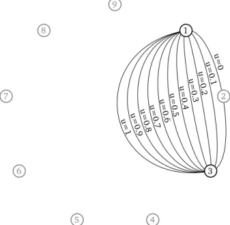
Fig. 1: Placement of a sample according to its utilisation
in the following section), but the basic mechanism used to create both types of TEED remains the same.
Let us assume that the TE algorithms under consideration operate on a weighted graph model G=(V,E) (each noden∈V
and each link l ∈ E). We also denote by c(l) and a(l) the capacity and available bandwidth respectively of linkl. So the link utilisation u(l) can be expressed as: c(l)−a(l)/c(l). Because TEED shows the ability of TE methods to balance incoming traffic we consider only nodes able to perform load balancing, i.e. those with node degree greater than one. Thus in the preliminary phase we recursively remove from the network graph all nodes with node degree equal to one. So for such a reduced network, before we start to draw the TEED, we need to collect samples of link utilisation u(l) of each link l ∈E. Various methods for collecting samples are described
in [9]. Here for simplicity we assume that periodic samples were collected.
Using the collected samples we can start to draw the TEED. In the first step all nodes are placed uniformly on the circumference of a circle. Then for each link utilisation sample u(l) we draw a curve between nodes interconnected by link l which curvature reflects the value of the sample. We assume that there is an attractor in the centre of of the nodes circle which attracts the line according to the value of the utilisation sample. So the higher value of the sample is, the more line is attracted to the centre, as shown in Figure 1. In current implementation we use Bezier curves to draw utilisation samples.
If the link utilisation is 0 the curve is placed on the circumference of the nodes circle, and if the link utilisation is1
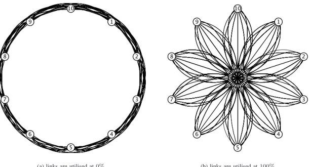
the curve passes through the centre of the circle. In Figure 2(a) we present a TEED for a full mesh topology with ten nodes (N = 10) when there is no traffic on any link, while in Figure 2(b) we show a TEED for the same topology when all links are utilised at 100%.
Such a design of TEED is simple and ensures that the eye is
open when links utilisation is low and closed when utilisation increases.
III. FUNCTIONALITY
The aim of TEED is to reflect the load balancing ability of Traffic Engineering algorithms. This can be achieved by generating a TEED when the offered load to the network is low. In such a case the eye should be wide open if the algorithm balances the load equally among available resources. If there are any lines going through the centre of TEED it means that some links are experiencing high load. This can be caused by two reasons — either the TE algorithm does not balance the incoming load well or some parts of the network carry more traffic because of irregularities in network toplogy. Although the TEED is most meaningful for lowly loaded networks, it can also provide insights when the load is high. In such a case the eye should be closed, and so to spot some abnormal behaviour we should look for lines which do not go through the centre of the eye. If such lines are observed then we have to check again if TE algorithm does not balance incoming load well or if it is because of the irregular network toplogy. However, occurrence of links which are underutilised when the load is high is obviously less problematic than congestion when we expect low loads. Therefore, TEED should be rather used for low loads than for high loads, but in this paper for most examples we present both cases.
If samples of link utilisation are collected quite frequently, after some time the TEED becomes unreadable due to too many lines being drawn on a single diagram. To be able to use TEED for a large number of samples we use a long-term TEED which does not draw a line for every sample, but groups similar samples and draws a line with a weight proportional to the population of the group. Thus we have two types of TEED:
short-term — these TEEDs are created simply by drawing a
line for each sample;
long-term — these TEEDs are created such that for a given
linklfirst all collected samples are grouped intoAclasses according to their value, and the size of a class equals to 1/A. For example, for A = 10 one class groups all samples with values from range (0−0.1) while in the next group all samples have values from(0.1−0.2), etc. Then for the considered link only A curves are drawn corresponding toA classes, and the width of each curve is proportional to the population of a class. To further increase readability we draw only lines corresponding to classes having highest population (which comprise altogether more than90%of all samples for a given link). Some examples of TEEDs are provided in Section V to illustrate their use in monitoring networks.
IV. SIMULATION ENVIRONMENT
In this paper we draw TEEDs for samples collected from simulations. In pracitce, such samples would be obtained from a real network, as described in the Introduction. The simula-tion model used in our experiment comprises the following components:
(a) links are utilised at0% (b) links are utilised at100%
Fig. 2: TEED for a network with full mesh topology, when no load is observed and when all links are congested
A. Traffic model
The connections arrive at each node independently accord-ing to a Poisson distribution with rateλand have exponentially distributed holding times with mean value 1/µ. The amount of bandwidth used by a connection is uniformly distributed over the interval: [64kb/s,6M b/s], with mean value B = 3.32M b/s. If N nodes in the network generate the traffic, the load offered to the network is [10] ρ = λN Bh′/µLC,
where h′ is the average shortest path distance between nodes,
calculated over all source-destination pairs. In our experiment we adjust λto produce the required offered load and fix the mean connection holding time at 180seconds.
B. Network topologies
We evaluate the functionality of TEEDs using various topologies, such as: the ISP [11]–[13] topology shown in Figure 3(a), the regular 4-ary 2-cube topology [10] shown in Figure 3(b), and a topology with two subnetworks intercon-nected by a direct link (1 hop) and a longer (3 hop) path, shown in Figure 3(c).
In all the networks we use bidirectional links, each with identical capacity C (C= 45M b/sas in DS-3 links).
C. Sample collection technique
In our simulations we collect samples periodically. Each minute we query each node about the utilisation of its outgoing links. On short-term TEEDs we draw samples corresponding to a five minute collection period, while on long-term TEEDs we present samples collected during one hour.
D. Routing algorithms
In this paper we compare two basic routing methods in creating TEEDs. We model the following routing algorithms:
shortest path (SP) algorithm — this selects the shortest
(min-hop) path, but if there are several such paths, we assume that the routing algorithm splits the load evenly across them (this is sometimes referred to as tie-breaking). Such an approach is used in OSPF [14] and it represents the typical routing method of todays Internet.
exponential cost function (EXP) algorithm — this selects the
least cost path, where the link cost is expressed as an exponential function of its utilisation. The choice of an exponential link cost function allows paths to avoid con-gested links [15]–[17]. We choose this as a representative of algorithms featuring load balancing capability.
V. EXAMPLES
TEEDs aim to visually present the load balancing ability of the algorithm. Therefore we first explore how the EXP algorithm performs load balancing on topologies featuring many paths between any source–destination pair. For this purpose we use the topologies shown in Figures 3(b) and 3(a). The topology shown in Figure 3(b) is very regular and is therefore especially useful to demonstrate how load balancing should work. Then in Section V-C using topology shown in Figure 3(c) we compare the SP algorithm and the EXP algorithm using corresponding TEEDs.
A. 4-ary 2-cube topology
For a network with a very regular topology such as the 4-ary 2-cube, TEEDs are clear and can be easily understood. In Figure 4 we observe that EXP balances the traffic well. For such regular topologies even the short-term TEED is sufficient to check if the algorithm is able to perform load balancing.
When we look at TEED when the network load is high (Figure 5), we also see that all links are evenly utilised, so the load is balanced well and there are no links which
4 17 16 15 14 13 12 11 10 9 8 7 6 5 4 3 2 1 18
(a) ISP (b) 4-ary 2-cube topology
13 12 11 10 9 8 7 6 5 4 3 2 1 (c) Two subnetworks
Fig. 3: Network topologies used to for TEEDs
(a) short-term TEED (b) long-term TEED
Fig. 4: TEEDs for 4-ary 2-cube topology, traffic loadρ= 0.2
are underutilised. Therefore, in such a simple case when the topology is regular and the algorithm performs load balancing the same conclusions can be drawn from short-term and long-term TEEDs (Figures 5(a) and 5(b) respectively). Moreover,
due to such regularities the diagrams presented for the 4-ary 2-cube topology are examples of perfect TEEDs, because when we increase the network load the eye closes uniformly from all directions. In the following sections we give examples of
(a) short-term TEED (b) long-term TEED
Fig. 5: TEEDs for 4-ary 2-cube topology, traffic loadρ= 0.7
less symmetric TEEDs, which feature irregularities due either to an irregular topology or to an unbalanced traffic pattern.
B. ISP topology
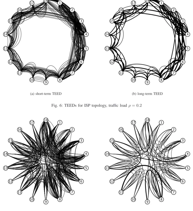
In this section we also observe that the EXP algorithm balances the load well for low and high loads (Figures 6 and 7 respectively). However, we notice irregularities in TEEDs due to irregular topology. Furthermore, for high load the long-term TEEDs (Figures 6(b) and 7(b)) provide additional information, because they allow us to observe which links carry more traffic than other links. Such information cannot be deducted from the short-term TEED (see Figure 7(a)). Therefore, we recommend the use of long-term TEEDs when we want to analyse the behaviour of a routing algorithm in detail, while the short-term TEEDs can be used to capture a snapshot of the distribution of incoming traffic.
C. Two subnetworks
In this section we try to show how TEED can be used to compare the load balancing ability of two routing algorithms. For this purpose we use the EXP algorithm and the SP algorithm. We use only the long-term TEEDs, because they make it easier to figure out which network links are used most heavily.
In Figure 8 we present a case when the network load is low. On the TEED of the EXP algorithm we can see that both paths between subnetworks (namely the 5–12–13–6 path and 5–6 path) are evenly utilised. However, the SP algorithm uses only the shortest path (5–6 path). So SP does not use both paths to balance traffic between two subnetworks. Moreover, the lines on the TEED of the EXP algorithm are much thicker than for the SP algorithm, what proves that the utilisation of these links is quite stable. The TEED of the SP algorithm has more thin lines, but instead the number of lines for each link is bigger than for the EXP algorithm, what informs us
that link utilisation fluctuates. Therefore we observe that the EXP algorithm balances the incoming traffic better than the SP algorithm.
In Figure 8 we present a case when the network load increases. Again we notice that the EXP algorithm uses both paths between subnetworks. Moreover, we can see that the load increases evenly on most of the links. For the TEED of the SP algorithm some links experience heavy traffic while some are underutilised. Therefore, we can say that the SP algorithm is not performing load balancing.
As we have demonstrated, using such a simple analysis based on long-term TEEDs we can compare TE methods. During such evaluation we have to watch for two things. Firstly, looking for lines which pass close to the centre of the eye allows us to identify congested regions of the network. Secondly, inspecting the line width allows us to check if traffic fluctuates — fewer but thicker lines usually mean more stable performance than numerous thin lines.
VI. NODE NAMING VARIANTS
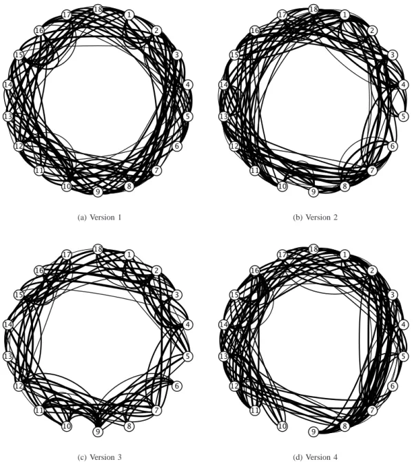
When TEEDs are created we assign an order number to each node. This assignment can be performed in an arbitrary way, but it does not influence the conclusions which can be drawn from obtained TEED. In Figure 10 we present four variants of a TEED obtained with different node number assignments. In all cases we observe that the load is balanced well and there is not abnormal congestion in any part of the network. Thus the observed performance does not change when we reassign node numbers. This characteristic was also observed for other node naming variants and for different topologies (results are not shown here). Thus it can be stated that TEEDs lead to the same conclusions regardless of the node naming variant used.
VII. STRENGTHS ANDWEAKNESSES The main weaknesses of TEEDs are:
6
(a) short-term TEED (b) long-term TEED
Fig. 6: TEEDs for ISP topology, traffic loadρ= 0.2
(a) short-term TEED (b) long-term TEED
Fig. 7: TEEDs for ISP topology, traffic loadρ= 0.7
• they are not readable for large networks. We believe that
it is better to use TEEDs for networks with less than 30 nodes.
• they only show the load balancing ability of the
al-gorithm. Sometimes it is not sufficient to balance the incoming traffic, or sometimes it is even better to restrict the TE method to use only short paths [18]. Therefore, to state which algorithm performs better we need also to evaluate other performace metrics.
Despite these weaknesses we think that TEEDs are useful because:
• they help to visualise the load balancing ability of TE
algorithms;
• they combine the virtues of commercial and research
performance analysis tools, allowing congested network regions to be identified and also allowing various algo-rithms to be compared;
• they provide an intuitive and easy-to-analyse form of
presenting information about traffic flowing through the network.
VIII. CONCLUSIONS
In this paper have proposed a new visualisation method called the Traffic Engineering Eye Diagram (TEED). It allows us to present the load balancing ability of Traffic Engineering methods in graphical form. It follows a simple mechanism — if network load is low the eye is open and when the load
(a) EXP algorithm (b) SP algorithm
Fig. 8: TEEDs for two subnetworks topology, traffic loadρ= 0.2
(a) EXP algorithm (b) SP algorithm
Fig. 9: TEEDs for two subnetworks topology, traffic loadρ= 0.5
increases the eye should gradually close. If the eye closes in an irregular way, it can be caused by poor load balancing or by an irregular network topology. However, if the load balancing works well and there are alternative paths between node pairs the eye should close uniformly from all directions.
Such a TEED can be helpful for researchers working on Traffic Engineering as well as network administrators mon-itoring network performance. It allows them to identify if the network load is spread evenly and moreover it provides a way to compare various TE methods. Thus it can help to monitor and analyse performance and furthermore to illustrate the impact of network topology on traffic distribution over the network.
REFERENCES
[1] J. Case, M. Fedor, M. Schoffstall, and J. Davin, “RFC 1157: A Simple Network Management Protocol (SNMP),” May 1990.
[2] Cisco NetFlow: http://www.cisco.com/warp/public/732/Tech/nmp/ netflow/.
[3] Multi Router Traffic Grapher: http://people.ee.ethz.ch/∼oetiker/ webtools/mrtg/.
[4] A. Feldmann, A. Greenberg, C. Lund, N. Reingold, and J. Rexford, “NetScope: Traffic engineering for IP networks,” IEEE Network Mag-azine, special issue on Internet Traffic Engineering, no. 2, pp. 11–19, March/April 2000.
[5] S. Suri, M. Waldvogel, and P. R. Warkhede, “Profile-Based Routing: A New Framework for MPLS Traffic Engineering,” in Quality of future Internet Services, ser. Lecture Notes in Computer Science, Berlin, September 2001, pp. 138–157.
[6] M. S. Kodialam and T. V. Lakshman, “Minimum Interference Routing with Applications to MPLS Traffic Engineering,” in Proceedings of INFOCOM 2000, Nineteenth Annual Joint Conference of the IEEE
8
(a) Version 1 (b) Version 2
(c) Version 3 (d) Version 4
Fig. 10: Long-term TEEDs for various node naming variants, ISP topology, traffic loadρ= 0.2
Computer and Communications Societies, Tel-Aviv, Israel, 2000, pp. 884–893.
[7] Q. Ma, “QoS Routing in the Integrated Services networks,” Ph.D. dissertation, School of Computer Science, Carnegie Mellon University, Pittsburgh, January 1998, CMU-CS-98-138.
[8] A. Elwalid, C. Jin, S. H. Low, and I. Widjaja, “MATE: MPLS adaptive traffic engineering,” in Proceedings of INFOCOM 2001, Twentieth Annual Joint Conference of the IEEE Computer and Communications Societies, Anchorage, Alaska, 2001, pp. 1300–1309.
[9] V. Paxson, G. Almes, J. Mahdavi, and M. Mathis, “RFC 2330: Frame-work for IP performance metrics,” May 1998.
[10] A. Shaikh, J. Rexford, and K. G. Shin, “Evaluating the Impact of Stale Link State on Quality-of-Service Routing,” IEEE/ACM Transactions on Networking (TON), vol. 9, no. 2, pp. 162–176, 2001.
[11] G. Apostopoulos, R. Guerin, S. Kamat, A. Orda, and S. K. Tripathi, “In-tradomain QoS Routing in IP Networks: A Feasibility and Cost/Benefit Analysis,” IEEE Network, vol. 13, no. 5, pp. 42–54, Sept./Oct. 1999. [12] X. Yuan and W. Zheng, “A Comparative Study of Quality of
Service Routing Schemes That Tolerate Imprecise State Information,” Florida State University Computer Science Department, Technical Report. [Online]. Available: http://websrv.cs.fsu.edu/research/reports/
TR-010704.pdf
[13] K. Kowalik and M. Collier, “ALCFRA — A Robust Routing Algorithm Which Can Tolerate Imprecise Network State Information,” in Proceed-ings of 15th ITC Specialist Seminar, Würzburg, Germany, July 2002, pp. 39–45.
[14] J. Moy, “RFC 2178: OSPF version 2,” July 1997.
[15] B. Awerbuch, Y. Azar, and S. A. Plotkin, “Throughput-Competitive On-line Routing,” in Proceedings of the 34th Annual Symposium on Foundations of Computer Science, Palo Alto, California, October 1993, pp. 32–40.
[16] R. Gawlick, A. Kamath, S. Plotkin, and K. Ramakrishnan, “Routing and Admission Control in General Topology Networks,” Technical Report STAN-CS-TR-95-1548, 1995.
[17] A. Kamath, O. Palmon, and S. Plotkin, “Routing and Admission Control in General Topology Networks with Poisson Arrivals,” in Proceedings of the 7th annual ACM-SIAM Symposium on Discrete algorithms, January 1996, pp. 269–278.
[18] Q. Ma and P. Steenkiste, “On path selection for traffic with bandwidth guarantees,” in Proceedings of IEEE International Conference on Net-work Protocols, Atlanta, GA, October 1997, pp. 191–202.