A Modified Simplex Method for Solving Linear-Quadratic
and Linear Fractional Bi-Level Programming Problem
Eghbal Hosseini
Ph.D. Candidate at Payamenur University of Tehran,
Department of Mathematics, Tehran, Iran
Isa Nakhai Kamalabadi
Professor of Industrial Engineeringat University of Kurdistan,
Sanandaj, Iran
ABSTRACT
The bi-level programming problem (BLP) is a suitable method for solving the real and complex problems in applicable areas such as management, economics, policies and planning and so on. There are several forms of the BLP as an NP-hard problem. The linear-quadratic bi-level programming (LQBP) and the linear-fractional bi-level programming (LFBP) are important forms of the BLP. In this paper, we attempt to develop two effective approaches, one based on modified simplex method and the other based on the genetic algorithm for solving the LQBP and LFBP. To obtain efficient upper bound and lower bound we employ the Karush -Kuhn -Tucker (KKT) conditions for transforming the LQBP into a single level problem. By using the proposed penalty functions, the single problem is transformed to an unconstraint problem and then it is solved by modified simplex method and genetic algorithm. The proposed approach achieves efficient and feasible solution and it is evaluated by comparing with references.
Keyword:
The linear-quadratic bi-level programming, the penalty function method, simplex method, Karush-Kuhn– Tucker conditions.1.
INTRODUCTION
al., 2008, Wan, et al., 2014, Xu, et al., 2014, Hosseini, E and I.Nakhai Kamalabadi., 2014, ) [18, 13, 17, 25, 27, 28, 10, 34], Primal–dual interior methods (Wend & U. P. Wen, 2000) [24], Enumeration methods (Thoai, et al., 2002) [22], Meta heuristic approaches (Hejazi, et al., 2002; Wang et al., 2008; Hu, et al., 2010; Baran Pal, et al., 2010; Wan et al., 2012; Yan, et al., 2013; Kuen-Ming et al., 2007, Hosseini, E and I.Nakhai Kamalabadi., 2013, He, X and C. Li, T. Huang, 2014) [11, 25, 12, 4, 26, 29, 14, 8, 9, 7]. In the following, these techniques are shortly introduced.
1.1. Transformation methods
An important class of methods for constrained optimization seeks the solution by replacing the original constrained problem with a sequence of unconstrained sub-problems or a problem with simple constraints. These methods are interested by some researchers for solving BLPP, so that they transform the follower problem by methods such as penalty functions, barrier functions, Lagrangian relaxation method or KKT conditions. In fact, these techniques convert the BLPP into a single problem and then it is solved by other methods [3, 4, 22, 23, 32].
1.2. Meta heuristic approaches
Meta heuristic approaches are proposed by many researchers to solve complex combinatorial optimization. Whereas these methods are too fast and known as suitable techniques for solving optimization problems, however, they can only propose a solution near to optimal. These approaches are generally appropriate to search global optimal solutions in very large space whenever convex or non-convex feasible domain is allowed. In these approaches, BLPP is transformed to a single level problem by using transformation methods and then meta heuristic methods are utilized to find out the optimal solution [15, 16, 17, 18, 19, 25, 33].
The remainder of the paper is structured as follows: in Section 2, basic concepts of the linear quadratic and linear fractional are introduced. The first presented algorithm is proposed in Section 3. In Section 4 and computational results are presented for approach in Section 5. Finally, the paper is finished in Section 6 by presenting the concluding remarks.
2.
The concepts of the problems
We research two special classes of bi-level programming: linear-quadratic bi-level programming (LQBP) and Linear-fractional bi-level programming (LFBP). The LQBP is formulated as follows [16]:
Where and f (x, y), g (x, y) are the objective functions of the leader and the follower, respectively. Also
is symmetric positive semi –definite matrix. Suppose that
Which
.
0
,
,
.
)
1
(
)
,
(
)
,
(
)
,
(
max
.
)
,
(
max
y
x
r
By
Ax
t
s
y
x
Q
y
x
y
d
x
c
y
x
g
t
s
y
b
x
a
y
x
f
T T T T T T
T y
T T x
2 1 2
1 n n n
n
R
R
Q
.
,
,
2 1 1 12 2
2 1
0
n n n
n n
n
R
Q
R
Q
R
Q
0 1
1 2
Q
Q
Q
Q
Q
T
,
,
c
R
n1Then the follower problem of the LQBP is
.
0
,
.
)
2
(
2
)
,
(
max
1 0
y
Ax
r
By
t
s
y
Q
y
xy
Q
y
d
y
x
g
T Ty
The LFBP problem is formulated as follows [21]:
Which
The feasible region of the LQBP and LFBP problems is
On the other hand if x be fixed, the feasible region of the follower can be explained as
Based on the above assumptions the follower rational reaction set is
Where the inducible region is as follows
Finally the bi-level programming problem can be written as
If there is finitesolution for the BLP problem, we define feasibility and optimality for the BLP problem as
)
4
(
.
}
0
,
,
|
)
,
{(
x
y
Ax
By
r
x
y
S
)
5
(
}.
0
,
,
|
{
)
(
x
y
By
r
Ax
x
y
S
)
6
(
)}.
(
|
)
,
(
max[
arg
|
{
)
(
x
y
y
g
x
y
y
S
x
P
)
7
(
)}.
(
,
)
,
{(
x
y
S
y
P
x
IR
)
8
(
}.
)
,
(
|
)
,
(
max{
f
x
y
x
y
IR
.
0
,
,
.
)
3
(
)
,
(
max
.
)
,
(
max
3 2 1
3 2 1
y
x
r
By
Ax
t
s
y
d
x
c
y
x
g
t
s
y
b
x
b
b
y
a
x
a
a
y
x
f
T T y
T T
T T
x
,
,
,
12 2
n
R
c
b
a
,
,
23 3
n
R
d
b
a
,
A
R
mn1,
,
2
n m
R
B
r
R
m,
,
x
R
n1y
R
n2.
,
,
11
b
R
Definition 1:
is a feasible solution to bi-level problem if
Definition 2:
is an optimal solution to the problem if
3.
Modified simplex algorithm by penalty function method for LQBP and
LFBP
Penalty functions transform a constrained problem into a single unconstrained problem or into a sequence of unconstrained problems. In this method the constraints are replaced into the objective function via a penalty parameter in a way that penalizes any violation of the constraints. In general, a suitable function must incur a positive penalty for infeasible points and no penalty for feasible points. Also the penalty function method is a common approach to solve the bi-level programming problems. In this kind of approach the lower level problem is appended to the upper level objective function with a penalty.
Since in problem (2), most of the equality constraints are not linear then it concerns that the above problem is non-convex programming, which indicates there are local optimal solutions that they are not global solution. Therefore solving the problem (2) is complicated and we use the following method for solving this problem.We use a penalty function to convert problem (2) to an unconstraint problem. Consider the problem (2), we append all constraints to the upper level objective function with a penalty for each constraint, then we obtain the following penalized problem.
Which N is a large positive number and M is a matrix of large positive numbers and
We now show that two problems (2), (11) have a same optimal solution according to the following theorem, and then solve the problem (11) instead problem (2) using proposed modified simplex method. Above method is satisfied for problem (3) too.
We now propose a theorem which establishes the convergence of algorithms for solving a problem of the form: minimize 𝑓(𝑥) subject to 𝑥 ∈ 𝑅𝑛. We show that an algorithm that generates n linearly independent search directions, and obtains a new point by sequentially minimizing f along these directions, converges to a stationary point. The theorem also establishes the convergence of algorithms using linearly independent and orthogonal search directions.
same optimal solution according to the following theorem.
Theorem 3.1:
Consider the following problem:
min 𝑥 𝑓(𝑥)
𝑠. 𝑡 𝑔𝑖 𝑥 ≤ 0, i=1,2,…,m,
(12)
.
)
,
(
x
y
IR
)
,
(
x
y
)
,
(
x
*y
*)
10
(
.
)
,
(
)
,
(
)
,
(
x
*y
*f
x
y
x
y
IR
f
)
9
(
}.
0
,
,
|
)
,
{(
x
y
Ax
By
r
x
y
S
.
0
,
,
,
,
)
11
(
.
)
(
)
2
2
(
max
1 0
w
v
u
y
x
r
w
By
Ax
t
s
vy
uw
N
d
v
Bu
y
Q
x
Q
M
y
b
x
a
T T.
2 1 n
𝑗 𝑥 = 0, j=1,2,…,l,
where 𝑓, 𝑔1, … , 𝑔𝑚, 1, … , 𝑙 are continuous functions on 𝑅𝑛 and 𝑋 is a nonempty set in 𝑅𝑛. Suppose that the problem
has a feasible solution, and 𝛼 is a continuous function as follows:
𝛼 x = 𝑚𝑖=1∅[𝑔𝑖(𝑥)]+ 𝑙𝑖=1∅[𝑖(𝑥)] (13)
where
∅ 𝑦 = 0 if y ≤ 0, ∅ 𝑦 > 0 𝑖𝑓 𝑦 > 0. (14)
∅ 𝑦 = 0 if y = 0, ∅ 𝑦 > 0 𝑖𝑓 𝑦 ≠ 0. (15)
Then,
inf 𝑓 𝑥 : 𝑔 𝑥 ≤ 0, 𝑥 = 0, 𝑥 ∈ 𝑋
= inf 𝑓 𝑥 + µ𝛼 𝑥 : 𝑥 ∈ 𝑋 (16)
where µ is a large positive constant (µ → ∞).
Proof:
Let y be a feasible point and . Let be an optimal solution to the problem to minimize subject to If , because are non-increasing functions, then, we must have
Now we show that By contradiction, suppose that, then
The above inequality is not possible in view of feasibility of y. thus, for all
Since is arbitrary, as
Since as then that is, is a optimal solution to the original problem and
that note that As
Both approach and hence, approaches zero. This completes the proof.
According to the above theorem two problems (2), (11) have a same optimal solution. The modified simplex method is proposed as follows.
Steps of the modified simplex algorithm are proposed as follows:
Let the main iteration number, k=0 and the objective function value at the optimal solution at the k-th iteration
1
x
0
)( )
(x x
f
xX, 1. 1 ( ) ( ) 21
f y f x
f
(
x
),
(
),
(
x
)
). ( ) (x f x1
f
.
)
(
x
,
)
(
x
(
x
)
0
.
,
(
x
)
0
,
(
x
)
0
x
)
(
)
(
sup
f
x
(
x
)
(
)
f
(
x
).
,
(
)
and
f
(
x
)
)
(
x
f
(
x
)
).
(
2
)
(
)
(
)
(
)
(
)
(
)
(
)
(
)
(
}
0
)
(
,
0
)
(
:
)
(
{
inf
1 1
1
y
f
x
f
y
f
x
f
x
x
f
x
x
f
x
h
x
g
x
f
.
2
)
(
)
(
1
1
f
y
f
x
(
x
)
0
.
Step 1:
If in the problem (11) is infeasible go to Step 5. Otherwise find an arbitrary basic feasible solution of Let be the associated basic inverses . The variables are divided in to two separate
classes, basic and non-basic variables that basic variables can be written according to the non-basic variables as follows:
Where are matrixes which correspond with the columns of the non-basic variables
respectively
.
Step 2:
By replacing equation into the objective function of the
problem (11), this objective function can be written as follows:
Which is the current value of the objective function. For all non-basic variables we calculate
According to the usual rule in the simplex method if all are positive, the simplex method will be finished and then we go to Step 4. Otherwise go to Step 3.
Step 3:
According to the usual rule in the simplex method enter the non-basic primal variable with the smallest or the non-basic dual variable with the largest into the basis. Also the leaving variable is determined using the usual minimum ratio rule:
Then go to Step 1.
Step 4:
If involves or N, go to Step 5. Otherwise let k=k+1, and go to Step 1.
Step 5:
If k=0 then the problem (11) is infeasible. Otherwise the obtained solution at the last iteration is the optimal solution.
4.
Computational results
Two following examples are solved by use of the genetic algorithm proposed in this article to illustrate the feasibility and efficiency of the proposed algorithm. The first example is LQBP and the second example is LFBP.
Example 1
Consider the following linear quadratic bi-level programming problem [16].
.
r
w
By
Ax
(
x
B,
y
B,
w
B)
r
w
By
Ax
1
H
)
(
1
N N N N N N
B B B
w
I
y
Q
x
P
b
H
w
y
x
i M *
k
Z *
0 Zk
Z
0
Z
z
j
c
j.
j j
c
z
)
(
)
2
2
(
1 00
a
x
b
y
M
Q
x
Q
y
Bu
v
d
N
uw
vy
z
z
T
T
N N N
Q
I
P
,
,
N N N
y
w
x
,
,
)
(
1
N N N N N N
B B B
w
I
y
Q
x
P
b
H
w
y
x
j j
c
z
j j
c
z
}
,
0
|
min{
y
j
N
y
r
y
r
ij ij i
kj
Using KKT conditions following problem is obtained:
Step 1: the following problem is feasible because (0, 0, 0, 0) is a feasible solution.
Now we find a basic feasible solution:
Therefore the associated basic inverses as follows:
Step 2: By replacing the basic variables into (21), the objective function is obtained.
Now we should calculate
for all non-basic variables:
Where
Step 3: According to (15), has the smallest therefore should be entered into the basis. Also the leaving variable is because of the usual minimum ratio rule:
Thus is substituted . Then go to Step 1.
Step 4: Because then k=k+1, and go to Step 1.
Now the first main iteration has been finished, but the algorithm has not been finished yet. Therefore we continue this process until the optimal solution is obtained after seven main iterations according to the Table 1.
0
0
0
0
,
4
5
2
12
1
0
0
0
0
1
0
0
0
0
1
0
0
0
0
1
,
,
,
2 1 2 1 1 4 3 2 1 8 7 6 5y
y
x
x
x
b
B
u
u
u
u
x
a
a
a
a
B
N B
1
0
0
0
0
1
0
0
0
0
1
0
0
0
0
1
1 1B
H
0
* 0
z
,
j jc
z
1
1 1 1 11
c
a
B
c
c
z
Bz
2
c
2
c
BB
1a
2
c
2
1
).
0
,
0
,
0
,
0
(
Bc
j jc
z
3x
x
3.
4
}
1
4
,
1
12
min{
}
,
min{
43 4 43 4 13 1y
r
y
r
y
r
4
u
3
x
u
40
* 0
z
z
0
z
*0
0
3
3 3 1 3
3
c
a
B
c
c
z
B 4 41
1 4
4
It is easy to show that by relaxing the u’s and v variables (by fixing them on zero or one) in the main problem, we can obtain upper bounds for the problem which might be not promising as expected. By enumeration of possible relaxation the best upper bound is shown in Table 1.
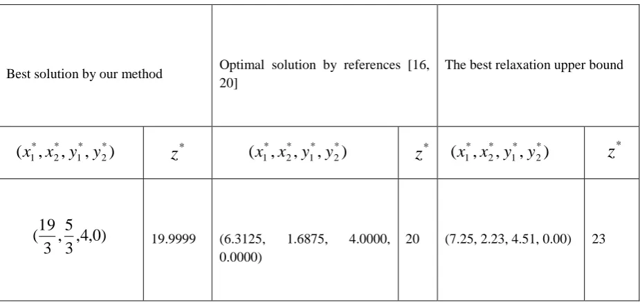
Table 1 comparison the best solutions - Example 1
According to the Table 1, the best solution by the proposed algorithm equals to the optimal solution exactly. It can be seen that the proposed method is efficient and feasible from the results.
Example 2
The following problem is linear fractional bi-level programming problem [13]. Best solution by our method Optimal solution by references [16,
20]
The best relaxation upper bound
19.9999 (6.3125, 1.6875, 4.0000, 0.0000)
20 (7.25, 2.23, 4.51, 0.00) 23
23
0
,
0
*2 1 4
3 2
1
w
w
w
v
v
z
w
.
0
,
,
3
4
,
13
2
,
26
2
2
,
32
3
2
,
28
4
,
15
3
5
.
max
.
2
2
5
max
y
x
y
x
y
x
y
x
y
x
y
x
y
x
t
s
y
t
s
y
x
y
x
y x
*
z
z
*z
*)
,
,
,
(
x
1*x
*2y
1*y
*2(
x
1*,
x
2*,
y
1*,
y
*2)
(
x
1*,
x
2*,
y
1*,
y
2*)
Appling KKT conditions the above problem convert to this problem:
By enumeration of possible relaxation, the best upper bound is
In genetic algorithm the initial population is created according to the proposed rules in section 4. Also the best solution is produced by the following chromosome:
0011100
Choosing by the proposed genetic algor ithm, the optimal solution is obtained. The best solution is and the upper level’s objective function is 1.66 also the lower level’s objective function is 8.66. The results are all close to the exact values in Ref [12, 21]. Behavior of the variables by modified simplex method has been show in figure 1.
5.
Conclusion and future work
In this paper, we used the KKT conditions to convert the problem into a single level problem. Then we presented a genetic method and a modified simplex method for solving linear-quadratic bi-level programming and linear-fractional bi-level programming problems. Comparing with the results of previous methods, both algorithms have better numerical results and present better solutions in much less times. The bestsolutions produced by proposed algorithms are feasible unlike the previous best solutions by other researchers.
In the future works, the following should be researched:
(1) Examples in larger sizes can be supplied to illustrate the efficiency of the proposed hybrid algorithm. (2) Research to use other unconstraint optimization methods such as Quasi – Newton for solving linear BLP.
.
6
,...,
1
,
0
,
,
,
,
,
0
,
0
,
3
4
2
3
4
3
,
3
4
,
13
2
,
26
2
2
,
32
3
2
,
28
4
,
15
3
5
.
2
2
5
max
6 6 5 5 4 4 3 3 2 2 1 1 6 5 4 3 2 1 6 5 4 3 2 1
i
u
w
v
y
x
yv
u
w
u
w
u
w
u
w
u
w
u
w
v
u
u
u
u
u
u
w
y
x
w
y
x
w
y
x
w
y
x
w
y
x
w
y
x
t
s
y
x
y
x
i i x,
0
,
0
,
0
3 4 56 2
1
u
u
w
w
w
v
u
95
.
1
0
,
0
,
0
5 6 *4 3 2
1
w
w
w
u
u
v
z
(3) Showing the efficiency of the proposed algorithms for solving other kinds of BLP.
6.
References
[1] Allende, G and B. G. Still, Solving bi-level programs with the KKT-approach, Springer and Mathematical Programming Society (2012) 1 31:37 – 48.
[2] Arora, S.R and R. Gupta, Interactive fuzzy goal programming approach for bi-level programming problem, European Journal of Operational Research (2007) 176 1151–1166.
[3] Bard, J.F, Some properties of the bi-level linear programming, Journal of Optimization Theory and Applications (1991) 68 371–378.
[4] Bard, J.F and Practical bi-level optimization: Algorithms and applications, Kluwer Academic Publishers, Dordrecht, 1998.
[5] Dempe, S and A.B. Zemkoho, On the Karush–Kuhn–Tucker reformulation of the bi-level optimization problem, Nonlinear Analysis 75 (2012) 1202–1218.
[6] Facchinei, F and H. Jiang, L. Qi, A smoothing method for mathematical programming with equilibrium constraints, Mathematical Programming 85 (1999) 107-134.
[7] He, X and C. Li, T. Huang, C. Li, Neural network for solving convex quadratic bilevel programming problems, Neural Networks, Volume 51, March 2014, Pages 17-25.
[8] Hosseini, E and I.Nakhai Kamalabadi, A Genetic Approach for Solving Bi-Level Programming Problems, Advanced Modeling and Optimization, Volume 15, Number 3, 2013.
[9] Hosseini, E and I.Nakhai Kamalabadi, Solving Linear-Quadratic Level Programming and Linear-Fractional Bi-Level Programming Problems Using Genetic Based Algorithm, Applied Mathematics and Computational Intellegenc, Volume 2, 2013.
[10] Hosseini, E and I.Nakhai Kamalabadi, Taylor Approach for Solving Non-Linear Bi-level Programming
Problem ACSIJ Advances in Computer Science: an International Journal, Vol. 3, Issue 5, No.11 , September 2014.
[11] Hejazi, S.R and A. Memariani, G. Jahanshahloo, (2002) Linear bi-level programming solution by genetic algorithm, Computers & Operations Research 29 1913–1925.
[12] Hu, T. X and Guo, X. Fu, Y. Lv, (2010) A neural network approach for solving linear bi-level programming problem, Knowledge-Based Systems 23 239–242.
[13] Khayyal, A.AL Minimizing a Quasi-concave Function Over a Convex Set: A Case Solvable by Lagrangian Duality, proceedings, I.E.E.E. International Conference on Systems, Man,and Cybemeties, Tucson AZ (1985) 661-663.
[14] Kuen-Ming, L and Ue-Pyng.W, Hsu-Shih.S, A hybrid neural network approach to bi-level programming problems, Applied Mathematics Letters 20 (2007) 880–884
[16] Masatoshi, S and Takeshi.M, Stackelberg solutions for random fuzzy two-level linear programming through possibility-based probability model, Expert Systems with Applications 39 (2012) 10898–10903.
[17] Mathieu, R. and L. Pittard, G. Anandalingam, Genetic algorithm based approach to bi-level Linear Programming, Operations Research (1994) 28 1–21.
[18] Nocedal, J and S.J. Wright, 2005 Numerical Optimization, Springer-Verlag, , New York.
[19] Pramanik, S and T.K. Ro, Fuzzy goal programming approach to multilevel programming problems, European Journal of Operational Research (2009) 194 368–376.
[20] Sakava, M. and I. Nishizaki, Y. Uemura, Interactive fuzzy programming for multilevel linear programming problem, Computers & Mathematics with Applications (1997) 36 71–86.
[21] Sinha, S Fuzzy programming approach to multi-level programming problems, Fuzzy Sets And Systems (2003) 136 189–202.
[22] Thoai, N. V and Y. Yamamoto, A. Yoshise, (2002) Global optimization method for solving mathematical programs with linear complementary constraints, Institute of Policy and Planning Sciences, University of Tsukuba, Japan 978.
[23] Vicente, L and G. Savard, J. Judice, Descent approaches for quadratic bi-level programming, Journal of Optimization Theory and Applications (1994) 81 379–399.
[24] Wend, W. T and U. P. Wen, (2000) A primal-dual interior point algorithm for solving bi-level programming problems, Asia-Pacific J. of Operational Research, 17.
[25] Wang, G. Z and Wan, X. Wang, Y.Lv, Genetic algorithm based on simplex method for solving Linear-quadratic bi-level programming problem, Computers and Mathematics with Applications (2008) 56 2550–2555.
[26] Wan, Z. G and Wang, B. Sun, ( 2012) A hybrid intelligent algorithm by combining particle Swarm optimization with chaos searching technique for solving nonlinear bi-level programming Problems, Swarm and Evolutionary Computation.
[27] Wan, Z and L. Mao, G. Wang, Estimation of distribution algorithm for a class of nonlinear bilevel programming problems, Information Sciences, Volume 256, 20 January 2014, Pages 184-196.
[28] Xu, P and L. Wang, An exact algorithm for the bilevel mixed integer linear programming problem under three simplifying assumptions, Computers & Operations Research, Volume 41, January 2014, Pages 309-318.
[29] Yan, J and Xuyong.L, Chongchao.H, Xianing.W, Application of particle swarm optimization based on CHKS smoothing function for solving nonlinear bi-level programming problem, Applied Mathematics and Computation 219 (2013) 4332–4339.
[30] Yibing, Lv and Hu. Tiesong, Wang. Guangmin , A penalty function method Based on Kuhn–Tucker condition for solving linear bilevel programming, Applied Mathematics and Computation (2007) 1 88 808–813.
[31] Zhang , G and J. Lu , J. Montero , Y. Zeng , Model, solution concept, and Kth-best algorithm for linear tri-level
, programming Information Sciences 180 (2010) 481–492
[33] Zheng, Y and J. Liu, Z. Wan, Interactive fuzzy decision making method for solving bi-level programming problem, Applied Mathematical Modelling, Volume 38, Issue 13, 1 July 2014, Pages 3136-3141.
[34] Hosseini, E and I.Nakhai Kamalabadi, Line Search and Genetic Approaches for Solving Linear Tri-level Programming Problem, International Journal of Management, Accounting and Economics Vol. 1, No. 4, November, 2014.