Available online throug
ISSN 2229 – 5046
COMPUTATIONAL STUDY OF NON-NEWTONIAN EYRING-POWELL FLUID FROM A
HORIZONTAL CIRCULAR CYLINDER WITH BIOT NUMBER EFFECTS
S. ABDUL GAFFAR
1*, V. RAMACHANDRA PRASAD
2, E. KESHAVA REDDY
1 1Department of Mathematics,
Jawaharlal Nehru Technological University Anantapur, Anantapuram-515002, India.
2
Department of Mathematics,
Madanapalle Institute of Technology and Science, Madanapalle-517325, India.
(Received On: 12-08-15; Revised & Accepted On: 28-09-15)
ABSTRACT
I
n this article, we investigate the nonlinear steady boundary layer flow and heat transfer of an incompressible Eyring-Powell non-Newtonian fluid from a Horizontal Circular Cylinder. The transformed conservation equations are solved numerically subject to physically appropriate boundary conditions using a second-order accurate implicit finite-difference Keller Box technique. The numerical code is validated with previous studies. The influence of a number of emerging non-dimensional parameters, namely the Eyring-Powell rheological fluid parameter (ε), the local non-Newtonian parameter based on length scale (δ), Prandtl number (Pr), Biot number (γ) and dimensionless tangential coordinate (ξ) on velocity and temperature evolution in the boundary layer regime are examined in detail. Furthermore the effects of these parameters on surface heat transfer rate and local skin friction are also investigated. Validation with earlier Newtonian studies is presented and excellent correlation achieved. It is found that the velocity and the Nusselt number (heat transfer rate) are reduced with increasing fluid parameter (𝜀𝜀), whereas temperature and skin friction are enhanced. Increasing fluid parameter, the local non-Newtonian parameter based on length scale (δ) enhances the velocity, local skin friction and the Nusselt number (heat transfer rate) but reduces the temperature. An increase in the Biot number (γ) is observed to enhance velocity, temperature, local skin friction and Nusselt number. An increasing Prandtl number, Pr, is found to decrease both velocity and temperature. The study is relevant to chemical materials processing applications.Keywords: Non-Newtonian Eyring-Powell model; Horizontal Cylinder; finite difference numerical method; heat
transfer; boundary layers; skin friction; Nusselt number; Biot number.
NOMENCLATURE
Cf skin friction coefficient
C fluid parameter
f non-dimensional steam function Gr Grashof number
g acceleration due to gravity k thermal conductivity of fluid Nu local Nusselt number Pr Prandtl number T temperature of the fluid
u, v non-dimensional velocity components along the x- and y- directions, respectively V velocity vector
x stream wise coordinate y transverse coordinate
Corresponding Author: S. Abdul Gaffar
1*,
1Department of Mathematics,
Greek
thermal diffusivity fluid parameter
non-dimensional concentration dimensionless radial coordinate dynamic viscosity
kinematic viscosity dimensionless temperature density of non-Newtonian fluid dimensionless tangential coordinate dimensionless stream function
ε fluid parameter γ Biot number
Subscripts
w conditions at the wall (cylinder surface)
∞ free stream conditions 1. INTRODUCTION
The dynamics of non-Newtonian fluids has been a popular area of research owing to ever-increasing applications in chemical and process engineering. Examples of such fluids include coal-oil slurries, shampoo, paints, clay coating and suspensions, grease, cosmetic products, custard, physiological liquids (blood, bile, synovial fluid) etc. The classical equations employed in simulating Newtonian viscous flows i.e. the Navier–Stokes equations fail to simulate a number of critical characteristics of non-Newtonian fluids. Hence several constitutive equations of non-Newtonian fluids have been presented over the past decades. The relationship between the shear stress and rate of strain in such fluids are very complicated in comparison to viscous fluids. The viscoelastic features in non-Newtonian fluids add more complexities in the resulting equations when compared with Navier–Stokes equations. Significant attention has been directed at mathematical and numerical simulation of non-Newtonian fluids. Recent investigations have implemented, respectively the Casson model [1], second-order Reiner-Rivlin differential fluid models [2], power-law nanoscale models [3], Eringen micro-morphic models [4] and Jefferys viscoelastic model [5].
Convective heat transfer has also mobilized substantial interest owing to its importance in industrial and environmental technologies including energy storage, gas turbines, nuclear plants, rocket propulsion, geothermal reservoirs, photovoltaic panels etc. The convective boundary condition has also attracted some interest and this usually is simulated via a Biot number in the wall thermal boundary condition. Recently, Ishak [6] discussed the similarity solutions for flow and heat transfer over a permeable surface with convective boundary condition. Aziz [7] provided a similarity solution for laminar thermal boundary layer over a flat surface with a convective surface boundary condition. Aziz [8] further studied hydrodynamic and thermal slip flow boundary layers with an iso-flux thermal boundary condition. The buoyancy effects on thermal boundary layer over a vertical plate subject a convective surface boundary condition was studied by Makinde and Olanrewaju [9]. Further recent analyses include Makinde and Aziz [10]. Gupta
et al. [11] used a variational finite element to simulate mixed convective-radiative micropolar shrinking sheet flow with a convective boundary condition. Swapnaet al. [12] studied convective wall heating effects on hydromagnetic flow of a micropolar fluid. Makinde et al. [13] studied cross diffusion effects and Biot number influence on hydromagnetic Newtonian boundary layer flow with homogenous chemical reactions and MAPLE quadrature routines. Bég et al. [14] analyzed Biot number and buoyancy effects on magnetohydrodynamic thermal slip flows. Subhashini et al. [15] studied wall transpiration and cross diffusion effects on free convection boundary layers with a convective boundary condition.
An interesting non-Newtonian model developed for chemical engineering systems is the Eyring-Powell fluid model. This rheological model has certain advantages over the other non-Newtonian formulations, including simplicity, ease of computation and physical robustness. Furthermore it is deduced from kinetic theory of liquids rather than the empirical relation. Additionally it correctly reduces to Newtonian behavior for low and high shear rates [16]. Several communications utilizing the Eyring–Powell fluid model have been presented in the scientific literature. Zueco and Bég [17] numerically studied the pulsatile flow of Eyring–Powell model using the network electro-thermal solver code, PSPICE. Islam et al. [18] derived Homotopypertubation solutions for slider bearings lubricated with Eyring-Powell fluids. Patel and Timol [19] numerically examined the flow of Eyring–Powell fluids from a two-dimensional wedge. Further investigations implementing the Eyring-Powell model in transport phenomena include Sirohi et al. [20] for wedge flows, Akbar et al. [21] for peristaltic thermal convection flows of reactive biofluids, Hayat et al. [22] for Sakiadis flows, Etchart [23] for entry length pipe flows and Hassanien and Hady [24] for magneto-convective flows.
α
β
φ
η
µ
ν
Sirohiet al. [25] used orthogonal collocation, asymptotic and transformation methods to simulate Eyring-Powell flow from an accelerated sheet. The Eyring-Powell model was also deployed by Yürüsoy [26] to investigate bearing tribological flows, by Ai and Vafai [27] to simulate Stokesian impulsively-started plate flows and also by Adesanya and Gbadeyan [28] for channel flows.
In many chemical engineering and nuclear process systems, curvature of the vessels employed is a critical aspect of optimizing thermal performance. Examples of curved bodies featuring in process systems include torus geometries, wavy surfaces, cylinders, cones, ellipses, oblate spheroids and in particular, spherical geometries. A number of theoretical and computational studies have been communicated on transport phenomena from cylindrical bodies, which frequently arise in polymer processing systems. These Newtonian studies were focused more on heat transfer aspects and include Eswara and Nath [29], Rotte and Beek [30] and the pioneering analysis of Sakiadis [31]. Further more recent studies examining multi-physical and chemical transport from cylindrical bodies include Zueco et al. [32, 33]. An early investigation of rheological boundary layer heat transfer from a horizontal cylinder was presented by Chen and Leonard [34] who considered the power-law model and demonstrated that the transverse curvature has a strong effect on skin friction at moderate and large distances from the leading edge of the boundary layer. Lin and Chen [35] also studied axisymmetric laminar boundary-layer convection flow of a power-law non-Newtonian fluid over both a circular cylinder and a spherical body using the Merk-Chao series solution method. Pop et al. [36] simulated numerically the steady laminar forced convection boundary layer of power-law non-Newtonian fluids on a continuously moving cylinder with the surface maintained at a uniform temperature or uniform heat flux. Further non-Newtonian models employed in analyzing convection flows from cylinders include micropolar liquids [37], viscoelastic materials [38, 39], micropolar nanofluids [40] and Casson fluids [41].
The objective of the present study is to investigate the laminar boundary layer flow and heat transfer of an Eyring-Powell non-Newtonian fluid from a horizontal circular cylinder. The non-dimensional equations with associated dimensionless boundary conditions constitute a highly nonlinear, coupled two-point boundary value problem. Keller’s implicit finite difference “box” scheme is implemented to solve the problem [42]. The effects of the emerging thermophysical parameters, namely the rheological parameters (𝜀𝜀, 𝛿𝛿), Biot number (𝛾𝛾) and Prandtl number (Pr), on the velocity, temperature, local skin friction, and heat transfer rate (local Nusselt number) characteristics are studied. The present problem has to the authors’ knowledge not appeared thus far in the scientific literature and is relevant to polymeric manufacturing processes in chemical engineering.
2. NON-NEWTONIAN CONSTITUIVE EYRING-POWELL FLUID MODEL
In the present study a subclass of non-Newtonian fluids known as the Eyring-Powell fluid is employed owing to its simplicity. The Cauchy stress tensor, in an Eyring-Powell non-Newtonian fluid [16] takes the form:
1
1
1
sinh
i i
ij
j j
u
u
x
C x
τ
µ
β
−
∂
∂
=
+
∂
∂
(1)whereµ is dynamic viscosity, 𝛽𝛽 and C are the rheological fluid parameters of the Eyring-Powell fluid model. Considering the second-order approximation of the sinh-1 function as:
3
1
1
1
1 1
1
sinh
,
1,
6
i i i i
j j j j
u
u
u
u
C x
C x
C x
C x
−
∂
≅
∂
−
∂
∂
∂
∂
∂
∂
(2)
The introduction of the appropriate terms into the flow model is considered next. The resulting boundary value problem is found to be well-posed and permits an excellent mechanism for the assessment of rheological characteristics on the flow behaviour.
3. MATHEMATICAL FLOW MODEL
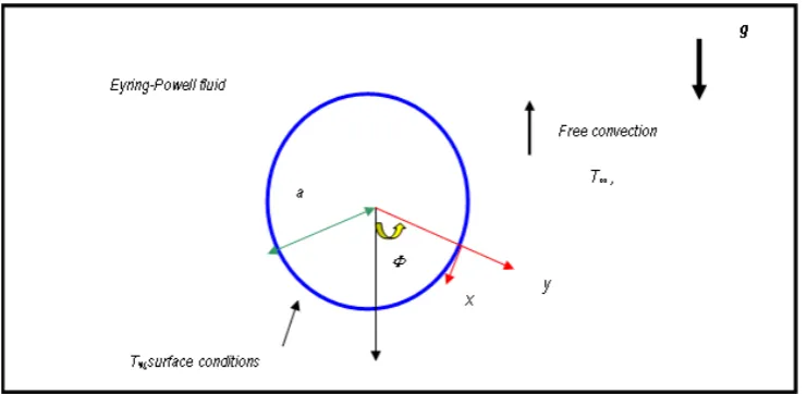
Steady, double-diffusive, laminar, incompressible flow of an Eyring-Powell fluid from a horizontal cylinder, is considered, as illustrated in Figure 1. The x-coordinate (tangential) is measured along the circumference of the horizontal cylinder from the lowest point and the y-coordinate (radial) is directed perpendicular to the surface, with a
denoting the radius of the horizontal cylinder. is the angle of the y-axis with respect to the vertical . The gravitational acceleration g, acts downwards. We also assume that the Boussineq approximation holds i.e. that density variation is only experienced in the buoyancy term in the momentum equation.
x a
Φ =
Figure 1: Physical model and coordinate system
Both horizontal cylinder and Eyring-Powell fluid are maintained initially at the same temperature. Instantaneously they
are raised to a temperature the ambient temperature of the fluid which remains unchanged. In line with the
approach of Yih [43] and introducing the boundary layer approximations, the equations for mass, momentum, and energy, can be written as follows:
0
u
v
x
y
∂
∂
+
=
∂
∂
(3)(
)
2
2 2
1
2 3 2
1
1
sin
2
u
u
u
u
u
x
u
v
g
T
T
x
y
ν
ρβ
C
y
ρβ
C
y
y
β
a
∞
∂
+
∂
=
+
∂
−
∂
∂
+
−
∂
∂
∂
∂
∂
(4)2 2
T
T
T
u
v
x
y
α
y
∂
+
∂
=
∂
∂
∂
∂
(5)Where u and vare the velocity components in the x - and y - directions respectively, is the kinematic viscosity of the Eyring-Powell fluid,
1
β
is the coefficient of thermal expansion. The Eyring-Powell fluid model therefore introduces a mixed derivative (second order, second degree) into the momentum boundary layer equation (4). The non-Newtonian effects feature in the shear terms only of eqn. (4) and not the convective (acceleration) terms. The third term on the right hand side of eqn. (4) represents the thermal buoyancy force and couples the velocity field with the temperature field equation (5)(
)
At
y
0,
u
0,
v
0,
k
T
h
wT
wT
y
∂
=
=
=
−
=
−
∂
As
y
→ ∞
,
u
→
0,
T
→
T
∞ (6)Here is the free stream temperature,
h
wis the convective heat transfer coefficient,T
wis the convective fluidtemperature.
The stream function ψ is defined by
u
y
∂ψ
=
∂
andv
x
∂ψ
= −
∂
, and therefore, the continuity equation is automaticallysatisfied. In order to render the governing equations and the boundary conditions in dimensionless form, the following non-dimensional quantities are introduced.
( )
(
)
1/ 4 1/ 4
3 2
1 3/ 2
2 2 4
,
,
,
,
, Pr
,
1
,
,
2
w wT T
x
y
Gr
f
Gr
a
a
T
T
g
T
T
a
Gr
Gr
C
C a
ψ
ν
ξ
η
θ ξ η
νξ
α
β
ε
δ
ν
ν
µβ
− ∞ ∞ ∞−
=
=
=
=
=
−
−
=
=
=
(7)w
T
>
T
∞,
µ
ν
ρ
=
All terms are defined in the nomenclature. In view of the transformation defined in eqn. (7), the boundary layer eqns. (4)-(6) are reduced to the following coupled, nonlinear, dimensionless partial differential equations for momentum and energy for the regime:
(
)
( )
2 2( )
2sin
'
1
ε
f
'''
ff
''
f
'
εδξ
f
''
f
'''
θ
ξ
ξ
f
'
f
f
''
f
ξ
ξ
ξ
∂
∂
+
+
−
−
+
=
−
∂
∂
(8)
''
'
'
'
Pr
f
f
f
θ
θ
ξ
θ
θ
ξ
ξ
∂
∂
+
=
−
∂
∂
(9)The transformed dimensionless boundary conditions are:
'
0,
0,
'
0,
1
At
η
f
f
θ
θ
γ
=
=
=
= +
,
'
0,
0
As
η
→ ∞
f
→
θ
→
(10)Here primes denote the differentiation with respect to and
ah
wGr
1/ 4k
γ
=
−is the Biot number. The wall thermal
boundary condition in (10) corresponds to convective cooling. The skin-friction coefficient (shear stress at the cylinder surface) and Nusselt number (heat transfer rate) can be defined using the transformations described above with the following expressions.
(
)
(
)
33/ 4 3
1
''( , 0)
''( , 0)
3
fGr
−C
= +
ε ξ
f
ξ
−
δ
εξ
f
ξ
(11)1/ 4
'( , 0)
Gr
−Nu
= −
θ ξ
(12)The location, ξ∼ 0, corresponds to the vicinity of the lower stagnation point on the cylinder. Since → 0/ 0 i.e. 1. For this scenario, the model defined by eqns. (8) to (9) contracts to an ordinary differential boundary value problem:
(
)
( )
21
+
ε
f
'''
+
ff
''
−
f
'
+ =
θ
0
(13)1
''
'
0
Pr
θ
+
f
θ
=
(14)The general model is solved using a powerful and unconditionally stable finite difference technique introduced by Keller [44]. The Keller-box method has a second order accuracy with arbitrary spacing and attractive extrapolation features.
4. NUMERICAL SOLUTION WITH KELLER BOX IMPLICT METHOD
The Keller-Box implicit difference method is implemented to solve the nonlinear boundary value problem defined by eqns. (8)–(9) with boundary conditions (10). This technique, despite recent developments in other numerical methods, remains a powerful and very accurate approach for parabolic boundary layer flows. It is unconditionally stable and achieves exceptional accuracy [44]. Recently this method has been deployed in resolving many challenging, multi-physical fluid dynamics problems. These include hydromagnetic Sakiadisflow of non-Newtonian fluids [45], nanofluid transport from a stretching sheet [46], radiative rheological magnetic heat transfer [47], waterhammer modelling [48], porous media convection [49] and magnetized viscoelastic stagnation flows [50]. The Keller-Box discretization is fully coupled at each step which reflects the physics of parabolic systems – which are also fully coupled. Discrete calculus associated with the Keller-Box scheme has also been shown to be fundamentally different from all other mimetic (physics capturing) numerical methods, as elaborated by Keller [44]. The Keller Box Scheme comprises four stages.
1) Decomposition of the Nth order partial differential equation system to N first order equations. 2) Finite Difference Discretization.
3) Quasilinearization of Non-Linear Keller Algebraic Equations and finally.
4) Block-tridiagonal Elimination solution of the Linearized Keller Algebraic Equations
η
sin
ξ
Stage 1: Decomposition of Nth order partial differential equation system to N first order equations
Equations (8) – (9) subject to the boundary conditions (10) are first cast as a multiple system of first order differential equations. New dependent variables are introduced:
( , )
', ( , )
'', ( , )
, ( , )
'
u x y
=
f
v x y
=
f
s x y
=
θ
t x y
=
θ
(15)These denote the variables for velocity, temperature and concentration respectively. Now Equations (8) – (9) are solved as a set of fifth order simultaneous differential equations:
(16)
(17)
(18)
(
)
2 2 2sin
1
ε
v
'
fv u
εδξ
v v
'
s
ξ
ξ
u
u
v
f
ξ
ξ
ξ
∂
∂
+
+
−
−
+
=
−
∂
∂
(19)'
Pr
f
t
s
ft
ξ
u
t
ξ
ξ
∂
∂
+
=
−
∂
∂
(20)Where primes denote differentiation with respect to the variable, η. In terms of the dependent variables, the boundary conditions assume the form:
'
0,
0,
'
0,
1
At
η
f
f
θ
θ
γ
=
=
=
= +
(21),
'
0,
0
As
η
→ ∞
f
→
θ
→
(22)Stage 2: Finite Difference Discretization
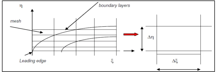
A two dimensional computational grid is imposed on the ξ-η plane as depicted in Fig.2. The stepping process is defined by:
(23)
(24)
Where is the spacing and is the spacing.
Figure 2: Keller box computational domain
If denotes the value of any variable at , then the variables and derivatives of Equations (16) – (20) at
are replaced by:
(25)
(26)
(27)
f
′ =
u
'
u
=
v
t
θ
′ =
0
0,
j j1h
j,
j
1, 2,..., ,
J
Jη
=
η
=
η
−+
=
η
≡
η
∞0 1
0,
n nk
n,
n
1, 2,...,
N
ξ
=
ξ
=
ξ
−+
=
n
k
∆ −
ξ
h
j∆ −
η
n j
g
(
η ξ
j,
n)
(
1/ 2)
1/ 2
,
n j
η
ξ
−−
(
)
1/ 2 1 1
1/ 2 1 1
1
,
4
n n n n n
j j j j j
g
−−=
g
+
g
−+
g
−+
g
−−(
)
1/ 2 1 1 1 1 1/ 21
,
2
nn n n n
j j j j
j j
g
g
g
g
g
h
η
− − − − − −
∂
=
−
+
−
∂
(
)
1/ 2 1 1 1 1 1/ 21
,
2
nn n n n
j j j j
n j
g
g
g
g
g
The finite-difference approximation of eqns, (16) – (20) for the mid-point , are: (28) (29) (30)
(
)
(
)
(
)
(
)(
)
(
)
(
)
(
)
(
) (
)
(
)
(
)
[ ]
21 1 1 1 1
2 1
2 1 1
1 1 1 1 1 1 1 /12
1
1
1
4
4
2
4
2
2
j j j
j j j j j j j j j j
n
j n j n
j j j j j j j j j j j
h
h
Bh
v
v
f
f
v
v
u
u
s
s
h
h
v
v
v
v
v
f
f
f
v
v
R
ε
α
α
α
α
εδ
ξ
− − − − − − − − − − − − − − −+
−
+ +
+
+
− +
+
+
+
−
+
−
+
+
−
+
=
(31)(
)
(
)
(
)(
)
(
)(
)
(
)
(
)
(
)
(
)
[ ]
11 1 1 1 1 1/ 2 1
1
1 1 1
1/ 2 1 1/ 2 1 1/ 2 1 2 1/ 2
1
1
Pr
4
4
2
2
2
2
j j j n
j j j j j j j j j j j j j
n
j n j n j n
j j j j j j j j j j
h
h
h
t
t
f
f
t
t
u
u
s
s
s
u
u
h
h
h
u
s
s
f
t
t
t
f
f
R
α
α
α
α
α
α
− − − − − − − − − − − − − − − − − − −
−
+ +
+
+
−
+
+
+
+
−
+
−
+
+
+
=
(32)Where we have used the abbreviations
, (33)
[ ]
(
)( )
(
)
(
)
(
)
( )
( )
2
1 1 1 1
1/ 2 1/ 2 1/ 2 1/ 2
1
1 1/ 2 1 2 2 1 1
1/ 2 1/ 2 1/ 2
1
'
1
1
'
n n n n
j j j
j n
j n
j n n
j j j
v
f
v
u
R
h
Bs
v
v
ε
α
α
εδξ
− − − − − − − − − − − − − − − −
+
+ −
− −
= −
+
−
(34)[ ]
1( )
1(
)
1 1 1 12 1/ 2 1/ 2 1/ 2 1/ 2 1/ 2 1/ 2
1
'
1
Pr
n n n n n n
j j j j j
j j
R
−−= −
h
t
−−+ −
α
f
−−t
−−+
α
u
−−s
−−
(35)The boundary conditions are:
0 0
0,
01,
0,
0,
0
n n n n n n
J J J
f
=
u
=
s
=
u
=
v
=
s
=
(36)Stage 3: Quasilinearization of Non-Linear Keller Algebraic Equations Assuming
f
jn 1, u
nj 1, v
nj 1, s
nj 1, t
nj 1− − − − − to be known for , then Eqns. (28) – (32) constitute a system of 5J+5 equations for the solution of 5J+5 unknowns
f
jn, u , v , s , t
nj nj nj nj, j = 0, 1, 2 …, J. This non-linear system of algebraic equations is linearized by means of Newton’s method as explained in [42, 44].Stage 4: Block-tridiagonal Elimination Solution of Linear Keller Algebraic Equations
The linearized system is solved by the block-elimination method, since it possesses a block-tridiagonal structure. The bock-tridiagonal structure generated consists of block matrices. The complete linearized system is formulated as a
block matrix system, where each element in the coefficient matrix is a matrix itself, and this system is solved using the efficient Keller-box method. The numerical results are strongly influenced by the number of mesh points in both
directions. After some trials in the η-direction (radial coordinate) a larger number of mesh points are selected whereas
in the ξ direction (tangential coordinate) significantly less mesh points are utilized. ηmax has been set at 25 and this
defines an adequately large value at which the prescribed boundary conditions are satisfied. ξmaxis set at 3.0 for this
flow domain. Mesh independence is achieved in the present computations. The numerical algorithm is executed in
MATLAB on a PC. The method demonstrates excellent stability, convergence and consistency, as elaborated by Keller [44].
5. NUMERICAL RESULTS AND INTERPRETATION
Comprehensive solutions have been obtained and are presented in Tables 1-5 and Figs. 3 - 10. The numerical problem comprises two independent variables (ξ,η), two dependent fluid dynamic variables (f,θ) and five thermo-physical and
body force control parameters, namely, γ, δ, ε, Pr, ξ. The following default parameter values i.e. γ = 0.2, δ = 0.1,
(
1/ 2,
)
n j
η
−ξ
(
)
1
1 1/ 2
,
n n n
j j j j
h
−f
−
f
−=
u
−(
)
1
1 1/ 2
,
n n n
j j j j
h
−u
−
u
−=
v
−(
)
1
1 1/ 2
,
n n n
j j j j
h
−s
−
s
−=
t
−1/ 2
n
n
k
ξ
α
=
−(
)
1/ 2 1/ 2
sin
n nB
ξ
ξ
− −=
ε = 0.1, Pr = 7.0, ξ = 1.0 are prescribed (unless otherwise stated). Furthermore the influence of stream-wise (transverse) coordinate on heat transfer characteristics is also investigated.
In Tables 1 & 2, we present the influence of the Eyring-Powell fluid parameter, ε, on the skin friction and heat transfer rate, along with a variation in Prandtl number (Pr). With increasing ε, the skin friction is enhanced. The parameter ε is inversely proportional to the dynamic viscosity of the non-Newtonian fluid. There as ε is elevated, viscosity will be reduced and this will induce lower resistance to the flow at the surface of the cylinder i.e. accelerate the flow leading to an escalation of shear stress. Furthermore this trend is sustained at any Prandtl number. However an increase in Prandtl number markedly reduces the shear stress magnitudes. Similarly increasing ε, is observed to reduce heat transfer rates, again at all Prandtl numbers, whereas it strongly accentuates heat transfer rates. Magnitudes of shear stress are always positive indicating that flow reversal (backflow) never arises.
Tables 3 & 4 document results forthe influence of the local non-Newtonian parameter (based on length scale x)i.e. δ and also the Prandtl number (Pr) on skin friction and heat transfer rate. Skin friction is generally decreased with increasing δ. However heat transfer rate (i.e. local Nusselt number function) is found to be enhanced with increasing δ.
2 / 3 4 2
2
2
C
a
Gr
ν
δ
=
and inspection of this definition shows that the direct proportionality of δto kinematic viscosity(ν) (with all other parameters being maintained constant) will generate a strong resistance to the flow leading to a deceleration i.e. drop in shear stresses. Conversely the direct proportionality of δto Grashof number (Gr) will imply that thermal buoyancy forces are enhanced as δ increases and this will cause a boost in heat transfer by convection fromthe cylinder surface manifesting with the greater heat transfer rates observed in Tables 3 and 4. These tables also show that with an increase in the Prandtl number, Pr, the skin friction is also depressed whereas the heat transfer rate is elevated.
Table 5 presents the Keller box numerical values of the missing condition
f
′′
( , 0)
ξ
(in brackets) and skin frictionf
C
for various values of δ and ε. It is found that skin friction is reduced with increasing values of δ. Furthermore, the skin frictionC
f is observed to be increased with a rise in the Eyring-Powell fluid parameter (ε) for all values of thelocal non-Newtonian parameter (δ).
Figures 3(a) - 3(b) illustrates the effect of Eyring-Powell fluid parameter
ε
,on the velocity and temperature (θ) distributions through the boundary layer regime. Velocity is significantly decreased with increasingε
at larger distance from the cylinder surface owing to the simultaneous drop in dynamic viscosity. Conversely temperature is consistently enhanced with increasing values ofε
. The mathematical model reduces to the Newtonian viscous flow model asε
→ 0 andδ
→ 0. The momentum boundary layer equation in this case contracts to the familiar equation for Newtonian mixed convection from a plate, vizf
'''
(
1
ξ
cot
ξ
)
ff
''
f
/2θ
sin
ξ
ξ
f
'
f
'
f
''
f
ξ
ξ
ξ
∂
∂
+ +
−
+
=
−
∂
∂
. The thermalboundary layer equation (9) remains unchanged. In fig. 3b temperatures are clearly minimized for the Newtonian case (ε =0) and maximized for the strongest non-Newtonian case (ε = 1.5).
Figures 4(a) – 4(b) depict the velocity and temperature distributions with increasing local non-Newtonianparameter,
δ
. Very little tangible effect is observed in fig. 4a, although there is a very slight increase in velocity with increase inδ
. Similarly there is only a very slight depression in temperature magnitudes in Fig. 4(b) with a rise inδ
.Figures 5(a) - 5(b) depict the evolution of velocity and temperature (θ) functions with a variation in Biot number,
γ
. Dimensionless velocity component (fig. 5a) is considerably enhanced with increasingγ
.In fig. 5b, anincrease in Biot number is seen to considerably enhance temperatures throughout the boundary layer regime. For γ< 1
i.e. small Biot numbers, the regime is frequently designated as being “thermally simple” and there is a presence of more
uniform temperature fields inside the boundary layer and the cylinder solid surface. For γ> 1 thermal fields are anticipated to be non-uniform within the solid body. The Biot number effectively furnishes a mechanism for comparing the conduction resistance within a solid body to the convection resistance external to that body (offered by the surrounding fluid) for heat transfer. We also note that a Biot number in excess of 0.1, as studied in figs. 5a,b corresponds to a "thermally thick" substance whereas Biot number less than 0.1 implies a “thermally thin” material. Since γis inversely proportional to thermal conductivity (k), as γ increases, thermal conductivity will be reduced at the
( )
f
′
( )
f
′
( )
θ
cylinder surface and this will lead to a decrease in the rate of heat transfer from the boundary layer to within the cylinder, manifesting in a rise in temperature at the cylinder surface and in the body of the fluid- the maximum effect will be sustained at the surface, as witnessed in fig. 5b. However for a fixed wall convection coefficient and thermal
conductivity, Biot number as defined in
xh
wGr
1/ 4k
γ
=
−is also directly inversely proportional to the local Grashof
(free convection) number. As local Grashof number increases generally the enhancement in buoyancy causes a deceleration in boundary layer flows [51-53]; however as Biot number increases, the local Grashof number must decreases and this will induce the opposite effect i.e. accelerate the boundary layer flow, as shown in fig. 5a.
Figures 6(a) – 6(b) depicts the profiles for velocity and temperature for various values of Prandtl number, Pr.
It is observed that an increase in the Prandtl number significantly decelerates the flow i.e., velocity decreases. Also increasing Prandtl number is found to decelerate the temperature.
Figures 7(a) – 7(b) depict the velocity and temperature distributions with dimensionless radial coordinate,
for various transverse (stream wise) coordinate values, ξ. Generally velocity is noticeably lowered with increasing migration from the leading edge i.e. larger ξ values (figure 7a). The maximum velocity is computed at the lower stagnation point(ξ~0) for low values of radial coordinate (η). The transverse coordinate clearly exerts a significant influence on momentum development. A very strong increase in temperature (θ), as observed in figure 7b, is generated throughout the boundary layer with increasing ξ values. The temperature field decays monotonically. Temperature is maximized at the surface of the spherical body (η= 0, for all ξ) and minimized in the free stream (η= 25). Although the behaviour at the upper stagnation point (ξ~π) is not computed, the pattern in figure 6b suggests that temperature will continue to progressively grow here compared with previous locations on the cylinder surface (lower values of ξ).
Figures 8(a) - 8(b) show the influence of Eyring-Powell fluid parameter, εon dimensionless skin friction coefficient
(
)
( )
3(
( )
)
31
, 0
'''
, 0
3
f
δ
f
ε ξ
ξ
εξ
ξ
+
′′
−
and heat transfer rate at the cylinder surface. It isobserved that the dimensionless skin friction is increased with the increase in εi.e. the boundary layer flow is accelerated with decreasing viscosity effects in the non-Newtonian regime. Conversely the surface heat transfer rate is substantially decreased with increasing ε values. Decreasing viscosity of the fluid (induced by increasing the ε value) reduces thermal diffusion as compared with momentum diffusion. A decrease in heat transfer rate at the wall will imply less heat is convected from the fluid regime to the cylinder, thereby heating the boundary layer and enhancing temperatures.
Figures 9(a) - 9(b) illustrates the influence of the local non-Newtonian parameter, δ, on the dimensionless skin frictioncoefficient and heat transfer rate. The skin friction (fig. 9a) at the cylinder surface is accentuated with increasing δ, however only for very large values of the transverse coordinate, ξ. The flow is therefore strongly accelerated along the curved cylinder surface far from the lower stagnation point. Heat transfer rate (local Nusselt number) is enhanced with increasingδ, again at large values of ξ, as computed in fig.9b.
Figures10 (a) - 10(b) presents the influence of the Biot number, γ, on the dimensionless skin friction coefficient and heat transfer rate at the cylinder surface. The skin friction at the cylinder surface is found to be greatly increased with rising Biot number, γ. This is principally attributable to the decrease in Grashof (free convection) number which results in an acceleration in the boundary layer flow, as elaborated by Chen and Chen [53]. Heat transfer rate (local Nusselt number) is enhanced with increasing γ, at large values of ξ, as computed in fig.10(b).
6. CONCLUSIONS
Numerical solutions have been presented for the buoyancy-driven flow and heat transfer of Eyring-Powell flow external to a horizontal cylinder. The Keller-box implicit second order accurate finite difference numerical scheme has been utilized to efficiently solve the transformed, dimensionless velocity and thermal boundary layer equations, subject to realistic boundary conditions. Excellent correlation with previous studies has been demonstrated (see Appendix) testifying to the validity of the present code. The computations have shown that:
(I) Increasing Eyring-Powell fluid parameter, ε, reduces the velocity and skin friction (surface shear stress) and heat transfer rate, whereas it elevates temperatures in the boundary layer.
(II) Increasing local non-Newtonian parameter, δ, increases the velocity, skin friction and Nusselt number for all values of radial coordinate i.e., throughout the boundary layer regime whereas it depresses temperature. (III)Increasing Biot number, γ, increases velocity, temperature and skin friction (surface shear stress). (IV)Increasing Prandtl number, Pr, decreases velocity and temperature.
( )
f
′
( )
θ
( )
f
′
( )
θ
( )
(V) Increasing transverse coordinate (ξ) generally decelerates the flow near the cylinder surface and reduces momentum boundary layer thickness whereas it enhances temperature and therefore increases thermal boundary layer thickness in Eyring-Powell non-Newtonian fluids.
Generally very stable and accurate solutions are obtained with the present finite difference code. The numerical code is able to solve nonlinear boundary layer equations very efficiently and therefore shows excellent promise in simulating transport phenomena in other non-Newtonian fluids. It is therefore presently being employed to study micropolar fluids [11, 12] and viscoplastic fluids [54] which also simulate accurately many chemical engineering working fluids in
curved geometrical systems. 7. REFERENCES
1. V. Ramachandra Prasad, A SubbaRao, N Bhaskar Reddy, B Vasu and O Anwar Bég, Modelling laminar transport phenomena in a Casson rheological fluid from a horizontal circular cylinder with partial slip,
ProcIMechE Part E: J Process Mechanical Engineering (2013). DOI: 10.1177/0954408912466350.
2. M. Norouzi, M. Davoodi, O. Anwar Bég and A.A. Joneidi, Analysis of the effect of normal stress differences on heat transfer in creeping viscoelastic Dean flow, Int. J. Thermal Sciences69, 61-69 (2013). 3. M. J. Uddin, N. H. M. Yusoff, O. Anwar Bég and A. I. Ismail, Lie group analysis and numerical
solutions for non-Newtonian nanofluid flow in a porous medium with internal heat generation,
PhysicaScripta, 87 (14pp) (2013).
4. M.M. Rashidi, M. Keimanesh, O. Anwar Bég, T.K. Hung, Magneto-hydrodynamic biorheological transport phenomena in a porous medium: A simulation of magnetic blood flow control, Int. J. Numer. Meth.Biomed.Eng. 27, 805-821 (2011).
5. D. Tripathi, S.K. Pandey and O. Anwar Bég, Mathematical modelling of heat transfer effects on swallowing dynamics of viscoelastic food bolus through the human oesophagus, Int. J. Thermal Sciences, 70, 41-53 (2013).
6. A. Ishak, Similarity solutions for flow and heat transfer over a permeable surface with convective boundary condition, Appl. Math. Comput. 217 (2010) 837–842.
7. A. Aziz, A similarity solution for laminar thermal boundary layer over a flat plate with a convective surface boundary condition, Comm.Non. Sci. Num. Sim. 14 (2009) 064–1068.
8. A. Aziz, Hydrodynamic and thermal slip flow boundary layers over a flat plate with constant heat flux boundary condition, Comm. Non. Sci. Num. Sim. 15 (2010) 573–580.
9. O.D. Makinde, P.O. Olanrewaju, Buoyancy effects on thermal boundary layer over a vertical plate with a convective surface boundary condition, Trans. ASME J. Fluids Eng. 132 (2010) 044502-2.
10. O.D. Makinde, A. Aziz, MHD mixed convection from a vertical plate embedded in a porous medium with a convective boundary condition, Int. J. Therm. Sci. 49 (2010) 1813–1820.
11. D. Gupta, L. Kumar, O Anwar Bég and B. Singh, Finite element simulation of mixed convection flow of micropolar fluid over a shrinking sheet with thermal radiation, Proc. IMechE. Part E: J Process Mechanical Engineering (2013). DOI: 10.1177/0954408912474586.
12. G. Swapna, Lokendra Kumar, O. Anwar Bég and Bani Singh, Effect of thermal radiation on the mixed convection flow of a magneto-micropolar fluid past a continuously moving plate with a convective surface boundary condition, Meccanica (2013).in press
13. O. D. Makinde, K. Zimba, O. Anwar Bég, Numerical study of chemically-reacting hydromagnetic boundary layer flow with Soret/Dufour effects and a convective surface boundary condition, Int. J. Thermal and Environmental Engineering, 4, 89-98 (2012).
14. O. Anwar Bég, M.J. Uddin, M.M. Rashidi and N. Kavyani, Double-diffusive radiative magnetic mixed convective slip flow with Biot number and Richardson number effects, J. Engineering Thermophysics (2013). 15. S.V. Subhashini, N. Samuel, I. Pop, Double-diffusive convection from a permeable vertical surface under
convective boundary condition, Int. Commun. Heat Mass Transfer 38 (2011) 1183-1188.
16. R.E. Powell, H. Eyring, Mechanism for relaxation theory of viscosity, Nature 154 (1944) 427–428.
17. J. Zueco, O.A. Bég, Network numerical simulation applied to pulsatile non-Newtonian flow through a channel with couple stress and wall mass effects, Int. J. Appl. Math.Mech. 5 (2009) 1–16.
18. S. Islam, A. Shah, C.Y. Zhou, I. Ali, Homotopypertubation analysis of slider bearing with Powell–Eyring fluid, Z. Angew. Math. Phys. 60 (2009) 1178–1193.
19. M. Patel, M.G. Timol, Numerical treatment of Powell–Eyring fluid flow using method of asymptotic boundary conditions, Appl. Numer. Math. 59 (2009) 2584–2592.
20. V. Sirohi, M.G. Timol, N.L. Kalathia, Numerical treatment of Powell–Eyring fluid flow past a 90 degree wedge, Reg. J. Energy Heat Mass Transfer 6 (3) (1984) 219–228.
21. N. S. Akbar, S. Nadeem, T. Hayat, A. A. Hendi, Simulation of heating scheme and chemical reactions on the peristaltic flow of an Eyring-Powell fluid, Int. J. Numerical Methods for Heat & Fluid Flow, 22, 764-776 (2012).
23. D.Y. Etchart, A pipe entry length solution for heat transfer and flow in Powell-Eyring fluids with temperature-dependent viscosity and constant flux boundary, PhD Thesis, Oregon State University, USA (1971).
24. I.A. Hassanien and F.M. Hady, Hydromagnetic free convection and mass transfer flow of non-Newtonian fluid through a porous medium bounded by an infinite vertical limiting surface with constant suction, Astrophysics and Space Science, 116, 141-148 (1985).
25. V. Sirohi, M G Timol and N L Kalthia, Powell-Eyring model flow near an accelerated plate Fluid Dyn.Res.2, 193 (1987).
26. M. Yürüsoy, A Study of pressure distribution of a slider bearing lubricated with Powell-Eyring fluid, Turkish J. Engineering Envir. Sciences, 27, 299-304, (2003).
27. L. Ai and K. Vafai, An investigation of Stokes’ second problem for non-Newtonian fluids, Numerical Heat Transfer, Part A, 47, 955–980 (2005).
28. O. Adesanya and J. A. Gbadeyan, Adomian decomposition approach to steady viscoelastic fluid flow with slip through a planer channel, Int. J. Nonlinear Science, 9, 86-94 (2010).
29. Eswara, A.T. and Nath G., Unsteady forced convection laminar boundary layer flow over a moving longitudinal cylinder. Acta Mech., 93, 13-28 (1992).
30. Rotte, J. W. and Beek, W.J., Some models for the calculation of heat transfer coefficients to moving continuous cylinders. Chem. Eng. Sci., 24, 705-716 (1969).
31. Sakiadis, B.C., Boundary behavior on continuous solid surfaces, III The boundary layer on a continuous cylindrical surface. AIChE. J., 7: 467-472 (1961).
32. Zueco, J., O. Anwar Bég, Tasveer A. Bég and H.S. Takhar, Numerical study of chemically-reactive buoyancy-driven heat and mass transfer across a horizontal cylinder in a high-porosity non-Darcian regime, J. Porous Media,12, 519-535 (2009).
33. Zueco, J., O. Anwar Bég, H. S. Takhar and G. Nath, Network simulation of laminar convective heat and mass transfer over a vertical slender cylinder with uniform surface heat and mass flux, J. Applied Fluid Mechanics,4, 13-23 (2011).
34. Chen S.S. and Leonard R., The axisymmetrical boundary layer for a power-law non-Newtonian fluid on a slender cylinder, Chem. Eng. J., 3, 88-92 (1972).
35. Lin, F. N. and Chern, S. Y., Laminar boundary-layerflow of non-Newtonian fluid, Int. J. Heat Mass Transfer, 22, 1323-1329 (1979).
36. Pop, I., Kumari, M. and Nath, G., Non-Newtonian boundary layers on a moving cylinder. Int. J. Eng. Sci., 28, 303-312 (1990).
37. Chang, C.L., Buoyancy and wall conduction effects on forced convection of micropolar fluid flow along a vertical slender hollow circular cylinder, Int. J. Heat Mass Transfer, 49, 4932–4942 (2006).
38. Anwar, I., Amin, N. and Pop, I., Mixed convection boundary layer flow of a viscoelastic fluid over a horizontal circular cylinder, Int. J. Non-Linear Mechanics, 43, 814-821 (2008).
39. Kasim, A.R.M., Mohammad N.F. and S. Shafie,Effect of heat generation on free convection boundary layer flow of a viscoelastic fluid past a horizontal circular cylinder with constant surface heat flux, 5th Int. Conf. Research and Education in Mathematics (ICREM5), Bandung, Indonesia, 22–24 October (2011).
40. Rehman, M.A. and Nadeem, S, Mixed convection heat transfer in micropolar nanofluid over a vertical slender cylinder, Chin. Phys. Lett., 29, 124701 (2012).
41. Prasad, V.R., A. SubbaRao, N. Bhaskar Reddy, B. Vasu, O. Anwar Bég, Modelling laminar transport phenomena in a Casson rheological fluid from a horizontal circular cylinder with partial slip, ProcIMechE- Part E: J. Process Mechanical Engineering (2012).
42. V. R. Prasad, B. Vasu, O. Anwar Bég and D. R. Parshad, Thermal radiation effects on magnetohydrodynamic free convection heat and mass transfer from a sphere in a variable porosity regime, Comm. Nonlinear Science Numerical Simulation, 17, 654–671 (2012).
43. K.A. Yih, Viscous and Joule Heating effects on non-Darcy MHD natural convection flow over a permeable sphere in porous media with internal heat generation, International Communications in Heat and mass Transfer, 27(4), 591-600 (2000).
44. H.B. Keller, Numerical methods in boundary-layer theory, Ann. Rev. Fluid Mech. 10, 417-433 (1978). 45. M. Subhas Abel, P.S. Datti, N. Mahesha, Flow and heat transfer in a power-law fluid over a stretching sheet
with variable thermal conductivity and non-uniform heat source,Int. J. Heat Mass Transfer ,52, 2902-2913 (2009).
46. K. Vajravelu, K.V. Prasad, J. Lee, C. Lee, I. Pop and Rob. A. Van Gorder, Convective heat transfer in the flow of viscous Ag–water and Cu–water nanofluids over a stretching surface, Int. J. Thermal Sciences, 50, 843-851 (2011).
47. C-H. Chen, Magneto-hydrodynamic mixed convection of a power-law fluid past a stretching surface in the presence of thermal radiation and internal heat generation/absorption, Int. J. Non-Linear Mechanics, 44, 596-603 (2009).
48. Y.L. Zhangand K. Vairavamoorthy, Analysis of transient flow in pipelines with fluid–structure interaction using method of lines, Int. J. Num. Meth. Eng, 63, 1446-1460 (2005).
50. M. Kumari, G. Nath, Steady mixed convection stagnation-point flow of upper convected Maxwell fluids with magnetic field, Int. J. Nonlinear Mechanics, 44, 1048-1055 (2009).
51. J.N. Potter and N Riley, Free convection from a heated sphere at large Grashof number, J. Fluid Mechanics, 100, 769-783 (1980).
52. A. Prhashanna, R.P. Chhabra, Free convection in power-law fluids from a heated sphere, Chem. Eng. Sci., 65, 6190-6205 (2010).
53. H-T.Chen, C-K. Chen, Natural convection of a non-Newtonian fluid about a horizontal cylinder and a sphere in a porous medium, Int. Comm. Heat Mass Transfer, 15, 605–614 (1988).
54. O. Anwar Bég, D. Tripathi, J-L Curiel-Sosa and T-K Hung, Peristaltic propulsion of viscoplastic rheological materials, Advances in Biological Modelling, Editor- T.Y. Wu, Taylor and Francis, Philadelphia, USA (2014). 55. Merkin, J. H., “Free convection boundary layer on an isothermal horizontal cylinder”, ASME, paper no.
76-HT-16, (1976).
56. Nazar, R., Amin, N. and Pop, I., “Free convection boundary layer on an isothermal horizontal circular cylinder in a micropolar fluid” Heat transfer, Proceeding of the 12th int. conference (2002).
TABLES
Table-1: Values of Cf and Nu for differentε and Pr (δ = 0.1, γ = 0.2, ξ = 1.0)
Pr ε = 0.0 ε = 0.3 ε = 0.5 ε = 0.7
Cf Nu Cf Nu Cf Nu Cf Nu
7 0.3501 0.3966 0.3789 0.3758 0.3954 0.3647 0.4103 0.3552 10 0.3261 0.4403 0.3523 0.4165 0.3674 0.4034 0.3809 0.3930 15 0.3000 0.4946 0.3236 0.4670 0.3371 0.4525 0.3492 0.4400 20 0.2823 0.5362 0.3041 0.5058 0.3166 0.4898 0.3279 0.4761 25 0.2690 0.5705 0.2896 0.5378 0.3014 0.5206 0.3121 0.5058 50 0.2308 0.6891 0.2476 0.6484 0.2578 0.6270 0.2666 0.6088 75 0.2105 0.7679 0.2259 0.7220 0.2347 0.6979 0.2427 0.6774 100 0.1970 0.8287 0.2113 0.7787 0.2194 0.7525 0.2268 0.7303
Table-2: Values of Cf and Nu for differentε and Pr(δ = 0.1, γ = 0.2, ξ = 1.0)
Pr ε = 1.0 ε = 1.2 ε = 1.5
Cf Nu Cf Nu Cf Nu
7 0.4303 0.3430 0.4424 0.3360 0.4591 0.3267 10 0.3991 0.3792 0.4102 0.3713 0.4253 0.3608 15 0.3656 0.4242 0.3755 0.4151 0.3891 0.4032 20 0.3461 0.4588 0.3522 0.4488 0.3649 0.4358 25 0.3264 0.4872 0.3350 0.4766 0.3469 0.4626 50 0.2785 0.5859 0.2857 0.5728 0.2956 0.5557 75 0.2534 0.6517 0.2598 0.6370 0.2687 0.6177 100 0.2368 0.7024 0.2428 0.6864 0.2510 0.6655
Table-3: Values ofCf andNu for differentδ and Pr (ε = 0.1, γ = 0.2, ξ = 1.0)
Pr δ = 0.0 δ = 5 δ = 10 δ = 15
Cf Nu Cf Nu Cf Nu Cf Nu
Table-4: Values of Cf and Nu for differentδ and Pr (ε = 0.1, γ = 0.2, ξ = 1.0)
Pr δ = 20 δ = 30 δ = 40
Cf Nu Cf Nu Cf Nu
7 0.3579 0.3940 0.3567 0.3972 0.3557 0.4017 10 0.3336 0.4364 0.3326 0.4394 0.3328 0.4438 15 0.3070 0.4890 0.3063 0.4918 0.3056 0.4951 20 0.2889 0.5295 0.2883 0.5321 0.2878 0.5350 25 0.2754 0.5627 0.2749 0.5625 0.2744 0.5680 50 0.2363 0.6779 0.2361 0.6800 0.2358 0.6823 75 0.2155 0.7545 0.2153 0.7565 0.2151 0.7585 100 0.2017 0.8136 0.2016 0.8154 0.2014 0.8173
Table-5: Numerical Values of
f
′′
( , 0)
ξ
( in brackets) and skin friction coefficient Cffor different values of δ and εδ \ ԑ 0.0 0.2 0.4 0.6 0.8 1.0
0.0 0.3501 0.3699 (0.3083) 0.3874 (0.2767) 0.4031 (0.2519) 0.4173 (0.2318) 0.4304 (0.2152)
0.1 0.3501 0.3699 (0.3084) 0.3874 (0.2769) 0.4031 (0.2521) 0.4173 (0.2320) 0.4303 (0.2153)
0.2 0.3501 0.3699 (0.3086) 0.3873 (0.2771) 0.4030 (0.2523) 0.4172 (0.2322) 0.4303 (0.2155)
0.3 0.3501 0.3699 (0.3087) 0.3873 (0.2773) 0.4030 (0.2525) 0.4172 (0.2323) 0.4303 (0.2156)
0.4 0.3501 0.3699 (0.3089) 0.3873 (0.2775) 0.4029 (0.2526) 0.4172 (0.2325) 0.4302 (0.2158)
0.5 0.3501 0.3699 (0.3090) 0.3873 (0.2776) 0.4029 (0.2528) 0.4171 (0.2327) 0.4302 (0.2159)
0.6 0.3501 0.3698 (0.3092) 0.3872 (0.2778) 0.4029 (0.2530) 0.4171 (0.2328) 0.4302 (0.2161)
0.7 0.3501 0.3698 (0.3093) 0.3872 (0.2780) 0.4028 (0.2532) 0.4170 (0.2330) 0.4301 (0.2163)
0.8 0.3501 0.3698 (0.3095) 0.3872 (0.2782) 0.4028 (0.2536) 0.4170 (0.2332) 0.4301 (0.2164)
0.9 0.3501 0.3698 (0.3096) 0.3872 (0.2784) 0.4028 (0.2536) 0.4170 (0.2334) 0.4300 (0.2166)
1.0 0.3501 0.3697 (0.3098) 0.3871 (0.2786) 0.4028 (0.2538) 0.4170 (0.2335) 0.4300 (0.2167)
COMPARISON TABLE: In order to verify the accuracy of our present method, we have compared our results with those of Merkin [49] and Nazar et al. [50]. The present results are found to be in good agreement.
( )
1/ 4
'
, 0
Nu Gr
−= −
θ ξ
ξ
Merkin[55] Nazar et. al.[56] Present0 0.4214 0.4214 0.4215
π/6 0.4161 0.4161 0.4162
π/3 0.4007 0.4005 0.4006
π/2 0.3745 0.3741 0.3742
2π/3 0.3364 0.3355 0.3357 5π/6 0.2825 0.2811 0.2821
Source of support: Nil, Conflict of interest: None Declared