Research Article
a
August
2018
Computer Science and Software Engineering
ISSN: 2277-128X (Volume-8, Issue-8)
A High-Order Model for Forecasting Rice Production Based
on Combined Fuzzy Time Series and Particle Swarm
Optimization
Nghiem Van Tinh
Thai Nguyen University – Thai Nguyen University of Technology, Vietnam [email protected]
Abstract— Crop production is considered as one of the real world complex problem due to its non-deterministic nature and uncertain behavior. Particularly, forecasting of rice production for a lead year is pre-eminent for crop planning, agro based resource utilization and overall management of rice production. As such, main challenge in rice production forecasting is to generate realistic method that must be capable for handling complex time series data and generating forecasting with almost tiny error. However, first-order fuzzy time series models have proven to be insufficient for solving these problems for the best forecasting accuracy. For this reason, this paper presents a novel high-order model based on fuzzy time series (FTS) and particle swarm optimization (PSO) which overcomes the drawback mentioned above. First, the global information of fuzzy logical relationships is combined with the local information of latest fuzzy fluctuation to find the forecasting value in the defuzzification stage. Second, the particle swarm optimization technique is developed to adjust the lengths of intervals in the universe of discourse for the fuzzification stage. To illustrate the forecasting process and the effectiveness of the proposed model, two numerical datasets of average rice production of Viet Nam and enrolment of students of Alabama University are examined. The examined results show that the proposed model gets lower forecasting errors than those of other existing models
Keywords— Forecasting, FTS, high - order fuzzy relationships, particle swarm optimization, enrolments, rice production.
I. INTRODUCTION
For more than one decade, many forecasting models has successfully been used to deal with various domain problems, such as academic enrollments [1]-[9], crop production [10][11], stock markets [12]- [14]and temperature prediction [14][15]. The tradition forecasting methods cannot deal with forecasting problems in which the historical data needs to be represented by linguistic values. Fuzzy set theory was firstly presented by Zadeh [16] to handle problems with linguistic values. The concepts of fuzzy sets have been successfully adopted to time series by Song and Chissom [1]. They introduced both the time-invariant fuzzy time series [1] and the time-variant time series [2] model which use the max–min operations to forecast the enrolments of the University of Alabama. Unfortunately, their method needs max– min composition operations to deal with fuzzy rules. It takes a lot of computation time when fuzzy rule matrix is big. Therefore, Chen [4] proposed the first-order fuzzy time
ISSN(E): 2277-128X, ISSN(P): 2277-6451, pp. 75-84 present a new forecast method to solve the TAIFEX forecasting problem based on fuzzy time series and PSO algorithm [17][18]. Some other authors, propose some methods for the temperature prediction and the TAIFEX forecasting, based on two-factor fuzzy logical relationships [19] and use them in which combine with PSO algorithm in fuzzy time series [20]. In Addition, other hybrid techniques such as: Pritpal and Bhogeswar [21] presented a new model based on hybridization of fuzzy time series theory with artificial neural network (ANN). Matarneh et al. [22] use feed forward artificial neural network and fuzzy logic for weather forecasting achieve better results.
The above mentioned researches showed that the lengths of intervals and creating forecasting rules are two important issues considered to be serious influencing the forecasting accuracy and applied to different problems. However, most of the models were implemented for forecasting of other historical data and not rice production. In this paper, a forecasting model based on the fuzzy logical relationship groups and PSO is presented to forecast rice production for each year on basis of historical time series of rice data in Viet Nam. Firstly, a new forecasting rule which combines global information of fuzzy logical relationships with local information of latest fuzzy fluctuation is developed to find forecasting values. Then, the root mean square error (RMSE) value is applied to estimate the forecasting accuracy. Finally, a new hybrid forecasting model based on combined FTS and particle swarm optimization (PSO) is developed to adjust the length of each interval in the universe of discourse by minimizing RMSE value. The case study with the data of rice production of Viet Nam and the enrolment data at the University of Alabama show that the performance of proposed model is better than those of any existing models based on the high – order FTS.
The rest of this paper is organized as follows. In Section 2, a brief review of the basic concepts of FTS and particle swarm optimization algorithms are introduced. Section 3, first gives the details of fuzzy time series model based on the proposed forecasted rules to forecast rice production and then combines with the particle swam optimization algorithm to find the effective lengths of intervals in the universe of discourse during training phase. Section 4 evaluates the forecasting performance of the proposed method with the existing methods based on the enrolments data of the University of Alabama. Finally, Section 5 provides some conclusions
II. BASIC CONCEPTS OF FUZZY TIME SERIES AND ALGORITHMS
An easy way to comply with the conference paper formatting requirements is to use this document as a template and simply type your text into it.
A. Basic concepts of fuzzy time series
Conventional time series refer to real values, but fuzzy time series are structured by fuzzy sets [16]. Let U = {u1, u2, … , un} be an universal set; a fuzzy set Ai of U is defined as 𝐴𝑖 = { fA(u1)/u1+, fA(u2)/u2… + fA(un)/un}, where fA is a membership function of a given set A, fA :U[0,1],fA(ui)indicates the grade of membership of ui in the fuzzy set A, fA(ui) ϵ [0, 1], and 1≤ i ≤ n .
General definitions of FTS are given as follows:
Definition 1: Fuzzy time series [1], [2]
Let Y(t)(t = . . , 0, 1, 2 . . ), a subset of R, be the universe of discourse on which fuzzy sets fi(t) (i = 1,2 … ) are defined and if F(t)is a collection of f1 t , f2 t , … , then F(t)is called a fuzzy time series on Y(t)(t . . ., 0, 1,2 . ..). Here, F(t) is viewed as a linguistic variable and fi(t) represents possible linguistic values of F(t).
Definition 2: Fuzzy logic relationship(FLR) [2],[3]
If F(t) is caused by F(t-1) only, the relationship between F(t) and F(t-1) can be expressed by F(t − 1) → F(t). According to [2] suggested that when the maximum degree of membership of F(t) belongs toAi, F(t) is considered Aj.
Hence, the relationship between F(t) and F(t -1) is denoted by fuzzy logical relationship Ai → Aj where Ai and Aj refer to the current state or the left - hand side and the next state or the right-hand side of fuzzy time series.
Definition 3: 𝛾 - order fuzzy logical relationships [6]
Let 𝐹(𝑡) be a fuzzy time series. If 𝐹(𝑡)is caused by 𝐹(𝑡 − 1), 𝐹(𝑡 − 2), … , 𝐹(𝑡 − 𝛾 + 1) 𝐹(𝑡 − 𝑚) then this fuzzy relationship is represented by by 𝐹(𝑡 − 𝛾), … , 𝐹(𝑡 − 2), 𝐹(𝑡 − 1) → 𝐹(𝑡) and is called an 𝑚 - order fuzzy time series.
Definition 4: Fuzzy relationship group (FRG) [4]
Fuzzy logical relationships, which have the same left-hand sides, can be grouped together into fuzzy logical relationship groups. Suppose there are relationships such as follows:
𝐴𝑖 → 𝐴𝑘1 , 𝐴𝑖 → 𝐴𝑘2 , …….
ISSN(E): 2277-128X, ISSN(P): 2277-6451, pp. 75-84 B. Particle swarm optimization algorithm (PSO)
Kennedy and Eberhart Error! Reference source not found.proposed traditional particle swarm optimization (PSO) techniques for dealing with optimization problems, where a set of potential solutions is represented by a swarm of particles and each particle is move through the search space for search the optimal solution. When particles moving, all particles (i.e, N particles) have fitness values which are evaluated by fitness functions and the position of the best particle among all particles found so far is recorded and each particle keeps its personal best position which has passed previously. At each times of moving, each jth element in the velocity vector Vid = [𝑣𝑖𝑑 ,1, 𝑣𝑖𝑑 ,2, … , 𝑣𝑖𝑑 ,𝑛] and each element xid ,j in the position vectorXid= [𝑥𝑖𝑑,1, 𝑥𝑖𝑑,2, … , 𝑥𝑖𝑑 ,𝑛] of particle id are calculated as follows:
Vidk+1= ωk∗ V
idk + C1∗ Rand ∗ Pbest _id − xidk + C2∗ Rand ∗ Gbest − xidk (1)
xidk+1= xidk + xidk+1 (2)
𝜔𝑘 = 𝜔
𝑚𝑎𝑥 −𝑘∗( 𝜔𝑚𝑎𝑥𝑖𝑡𝑒𝑟 _𝑚𝑎𝑥−𝜔𝑚𝑖𝑛) (3)
The Pbest _id for jth particle is presented as 𝑃𝑏𝑒𝑠𝑡 _𝑖𝑑 = [ 𝑝𝑖𝑑 ,1, 𝑝𝑖𝑑 ,2, … , 𝑝𝑖𝑑 ,𝑛]and calculated as:
𝑃𝑏𝑒𝑠𝑡_𝑖𝑑𝑘+1 𝑓 𝑥 = 𝑃𝑏𝑒𝑠 𝑡𝑖𝑑
𝑘 +1 , 𝑖𝑓𝑓𝑖𝑡𝑛𝑒𝑠𝑠 𝑥
𝑖𝑑𝑘+1 > 𝑃𝑏𝑒𝑠 𝑡𝑖𝑑 𝑘
𝑓𝑖𝑡𝑛𝑒𝑠𝑠 𝑥𝑖𝑑𝑘+1 , 𝑖𝑓𝑓𝑖𝑡𝑛𝑒𝑠𝑠 𝑥
𝑖𝑑𝑘+1 ≤ 𝑃𝑏𝑒𝑠 𝑡𝑖𝑑
𝑘 (4)
The Gbest at kth iteration is computed as:
Gbest = min(𝑃𝑏𝑒𝑠 𝑡𝑘 𝑖𝑑) (5)
where Vidk is the velocity of the particle id in kth iteration, and is limited to [−Vmax, Vmax],Vmax is a constant pre-defined by user. Xidk is the current position of a particle id in kth iteration. The symbol 𝜔denotes the inertial weight coefficient. The symbols C1 and C2 denote the self-confidence coefficient and the social confidence coefficient, respectively. In a standard PSO, the value of 𝜔decreases linearly during the whole running procedure, and C1 = C2 = 2. The symbol Rand () denotes a function can generate a random real number between 0 and 1 under normal distribution. The symbols
Pbest_iddenotes the personal best position of the particle id, respectively. The symbol Gbest denotes the best one of all
personal best positions of all particles within the swarm. The whole running procedure of the standard PSO is described in Algorithm 1.
Algorithm 1: Standard PSO algorithm
1. Initialize the N particles‟ positions Xid and velocities Vid
2. While the stop condition (the optimal solution is found or the maximum moving step is reached) is not satisfied
do
2.1. For particle id, (1≤ id ≤ N) do
Calculate the fitness value of particle i
if fitness value better than previous Pbest _id then
Set fitness value is new Pbest _id according to (4) end if
end for
2.2. Update the global best position of all particles Gbest according to (5). 2.3. For particle i, (1≤ id ≤ N) do
Move particle id to another position according to (1) and (2) end for
2.4. Update 𝜔 according to Eq.(3) end while
III. A FORECASTING MODEL BASED ON THE FUZZY TIME SERIES AND PSO
A. Forecasted model based on the high–order FLRGs
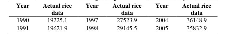
In the section, to verify the effectiveness of the proposed model, the annual data to represent the average rice production (thousand ton/ year) of Viet Nam between 1990-2010 is listed in Table 1 in which it taken from the site www.gso.gov.vn, more precisely from https://www.gso.gov.vn/default.aspx?tabid=717 is used to illustrate the first - order fuzzy time series forecasting process. The step-wise procedure of the proposed model is detailed as follows:
Table 1: The annual data of the average rice production (thousand ton/ year) of Viet Nam
Year Actual rice
data
Year Actual rice
data
Year Actual rice
data
1990 19225.1 1997 27523.9 2004 36148.9
ISSN(E): 2277-128X, ISSN(P): 2277-6451, pp. 75-84
1992 21590.4 1999 31393.8 2006 35849.5
1993 22836.5 2000 32529.5 2007 35942.7
1994 23528.2 2001 32108.4 2008 38729.8
1995 24963.7 2002 34447.2 2009 38950.2
1996 26396.7 2003 34568.8 2010 39988.9
Step 1:Define the universe of discourse U
Assume Y(t) be the historical data of rice production at year t ( 1990≤ 𝑡 ≤ 2010). The university of discourse is defined asU = Dmin, Dmax .In order to ensure the forecasting values bounded in the universe of discourse U, we set Dmin = Imin − N1 and Dmax = Imax + N2; where Imin, Imaxare the minimum and maximum data of Y t ; N1and N2are two proper positive to tune the lower bound and upper bound of the U. From the historical rice production data are shown in Table 1, we obtainImin = 19225.1 và Imax = 39988.9. Thus, the universe of discourse is defined as U= [ Imin− N1, Imax + N2]= [19000, 40000] with N1= 225.1 and N2= 11.1
Step 2: Partition U into equal length intervals
Divide U into equal length intervals. Compared to the previous models in [4], [17], we cut U into seven
intervals, u1, u2, . . . , u7, respectively. The length of each interval is L =
Dmax−Dmin 7 =
40000 −19000
7 = 3000. Thus, the seven intervals are defined as follows:
ui = (Dmin+ (i-1)*L, Dmin + i *L], with (1 ≤ 𝑖 ≤ 7) gets seven intervals as:
u1 = (19000, 22000], u2 = (22000, 25000], …, u6 = (34000, 37000], u7 = (37000, 40000].
Step 3: Define the fuzzy sets for observation of rice production
Each interval in Step 2 represents a linguistic variable of “rice production”. For seven intervals, there are seven linguistic values which are 𝐴1= “very poor rice production”, 𝐴2=“poor rice production”, 𝐴3=“ above poor rice production”, 𝐴4= “average rice production”, 𝐴5= “above average rice production”, 𝐴6= “good rice production”, and 𝐴7=“ very good rice production” to represent different regions in the universe of discourse on U, respectively. Each linguistic variable represents a fuzzy set 𝐴𝑖and its definitions is described in (6) as follows:
A1 = 1 𝑢1+
0.5 𝑢2+
0 𝑢3+ ⋯ +
0 𝑢7
A2 =0.5𝑢1+𝑢21 +0.5𝑢3+ ⋯ +𝑢70 (6)
--- A7 =𝑢10 +𝑢20 + ⋯ +0.5𝑢6+𝑢71
For simplicity, the membership values of fuzzy set Ai either are 0, 0.5 or 1. The value 0, 0.5 and 1 indicate the grade of membership of uj(1 ≤ j ≤ 7). in the fuzzy set Ai(1 ≤ i ≤ 7).
Where, where the symbol „+‟ denotes fuzzy set union, the symbol „/‟ denotes the membership of uj which belongs to Ai. Step 4: Fuzzify all historical data of rice production
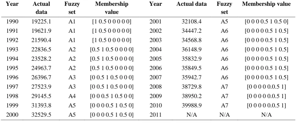
To fuzzify all historical data, it‟s necessary to assign a corresponding linguistic value to each interval first. The simplest way is to assign the linguistic value with respect to the corresponding fuzzy set that each interval belongs to with the highest membership degree. For example, the historical rice data of year 1990 is 19225.1, and it belongs to interval 𝑢1 because 19225.1 is within (19000, 22000]. So, we then assign the linguistic value „„very poor rice production” (eg. the fuzzy set 𝐴1) corresponding to interval 𝑢1 to it. Consider two time serials data 𝑌(𝑡) and 𝐹(𝑡) at year t, where 𝑌(𝑡) is actual data and 𝐹(𝑡) is the fuzzy set of 𝑌 𝑡 . According to formula (6), the fuzzy set 𝐴1 has the maximum membership value at the interval 𝑢1. Therefore, the historical data time series on date Y(1990) is fuzzified to 𝐴1. The completed fuzzified results of rice production are listed in Table 2.
Step 5:Define all 𝛾 – order fuzzy logical relationships.
Based on Definition 2. To establish a 𝛾 - order fuzzy relationship, we should find out any relationship which hasthe F t − 𝛾 , F t − 𝛾 + 1 , . . . , F t − 1 → 𝐹(𝑡), where F t − 𝛾 , F t − 𝛾 + 1 , . . . , F t − 1 and 𝐹(𝑡) are called the current state and the next state of fuzzy logical relationship, respectively. Then a 𝛾 - order fuzzy logic relationship in the training phase is got by replacing the corresponding linguistic values.
ISSN(E): 2277-128X, ISSN(P): 2277-6451, pp. 75-84
Table 2. The results of fuzzification for rice production data
Year Actual
data
Fuzzy set
Membership value
Year Actual data Fuzzy
set
Membership value
1990 19225.1 A1 [1 0.5 0 0 0 0 0] 2001 32108.4 A5 [0 0 0 0.5 1 0.5 0]
1991 19621.9 A1 [1 0.5 0 0 0 0 0] 2002 34447.2 A6 [0 0 0 0 0.5 1 0.5]
1992 21590.4 A1 [1 0.5 0 0 0 0 0] 2003 34568.8 A6 [0 0 0 0 0.5 1 0.5]
1993 22836.5 A2 [0.5 1 0.5 0 0 0 0] 2004 36148.9 A6 [0 0 0 0 0.5 1 0.5]
1994 23528.2 A2 [0.5 1 0.5 0 0 0 0] 2005 35832.9 A6 [0 0 0 0 0.5 1 0.5]
1995 24963.7 A2 [0.5 1 0.5 0 0 0 0] 2006 35849.5 A6 [0 0 0 0 0.5 1 0.5]
1996 26396.7 A3 [0 0.5 1 0.5 0 0 0] 2007 35942.7 A6 [0 0 0 0 0.5 1 0.5]
1997 27523.9 A3 [0 0.5 1 0.5 0 0 0] 2008 38729.8 A7 [0 0 0 0 0.0.5 1]
1998 29145.5 A4 [0 0 0.5 1 0.5 0 0] 2009 38950.2 A7 [0 0 0 0 0.0.5 1]
1999 31393.8 A5 [0 0 0 0.5 1 0.5 0] 2010 39988.9 A7 [0 0 0 0 0.0.5 1]
2000 32529.5 A5 [0 0 0 0.5 1 0.5 0] 2011 N/A N/A N/A
Table 3. The 2rd- order fuzzy logical relationships
No Fuzzy relations No Fuzzy relations No Fuzzy relations No Fuzzy relations
1 A1, A1 → A1 5 A2, A2 → A3 9 A4, A5 → A6 13 A6, A6 → A6
2 A1, A1 → A2 6 A2, A3 → A3 10 A5, A5 → A5 14 A6, A6 → A7
3 A1, A2 → A2 7 A3, A3 → A4 11 A5, A5 → A6 15 A6, A7 → A7
4 A2, A2 → A2 8 A3, A4 → A5 12 A5, A6 → A6 16 A7, A7 → A7
17 A7, A7 → #
Step 6: Establish all 𝛾 – order fuzzy logical relationshipsgroups
Based on [4]all the fuzzy relationships having the same fuzzy set on the left-hand side or the same current state can be put together into one fuzzy relationship group. The fuzzy logical relationship as the same are counted only once. Thus, from Table 3 and based on Definition 4, we can obtain seven 2rd – order fuzzy relationshipgroupsshown in Table 4.
Table 4: The complete result of the 2nd - order fuzzy relationship groups
No Fuzzy relation
group
No Fuzzy relation
groups
No Fuzzy relation
groups
No Fuzzy relation
groups
1 A1, A1 -> A1, A2 4 A2, A3 -> A3 7 A4, A5 -> A5 10 A6, A6 -> A6, A7
2 A1, A2 -> A2 5 A3, A3 -> A4 8 A5, A5 -> A5, A6 11 A6, A7 -> A7
3 A2, A2 -> A2, A3 6 A3, A4 -> A5 9 A5, A6 -> A6 12 A7, A7 -> #
Step 7: Calculate and defuzzify the forecasted output values
In this step, to enhance the forecasting accuracy, we propose a novel forecasting rule which combines the global information of fuzzy relationships with the local information latest fuzzy set appear in current state, named (ILF) to calculate the forecasting output valuesfor the trained patterns in the training phase. In addition to, we use13to calculate the forecasting output values for the untrained patterns in the testing phase
Rule 1: For the training phase, the forecasted value of rice production at year t is computed according to formula (7) as follows:
Forecasted_value = 𝑤1* Global_inf + 𝑤2* Local_inf (7)
Where,
The Global_inf is the global information which can be determined by the fuzzy groups created in Step 6. Supose that there is a 𝛾- order fuzzy relationship group is presented as follows: At−γ, At−γ+1,…, At−1→ At1, At2, … , Atp Base on Chen [ 1], the value of Global_inf is calculated as follows:
𝑮𝒍𝒐𝒃𝒂𝒍_𝒊𝒏𝒇 = 𝑚𝑡1+ 𝑚𝑡2+⋯+𝑚𝑡𝑝 𝑝
ISSN(E): 2277-128X, ISSN(P): 2277-6451, pp. 75-84
The Local_inf is the local information which is derived by the ILF scheme. The ILF scheme is an estimating scheme determined by the next state and the latest past in the current state. Suppose that there is a 𝛾- order fuzzy relationship as follows: At−γ, At−γ+1,…, At−1→ At1, At2, … , Atp. The Local_inf value is formulated as follows:
𝑳𝒐𝒄𝒂𝒍𝒊𝒏𝒇= 𝐿𝑣𝑡𝑘+
𝑈𝑣𝑡𝑘 − 𝐿𝑣𝑡𝑘
2 ∗
𝑚𝑡𝑘− 𝑚𝑡−1 𝑚𝑡𝑘+ 𝑚𝑡−1
Where, At−1 and Atk(1 ≤ 𝑘 ≤ 𝑝) denote the latest past in the current state and the next state, respectively.
Here, 𝑚𝑡−1 and 𝑚𝑡k are midpoints of the fuzzy intervals 𝑢𝑡−1 and 𝑢𝑡k with respective to At−1 and Atk; 𝐿𝑣𝑡𝑘, 𝑈𝑣𝑡𝑘 denote the lower bound and upper bound of interval 𝑢𝑡k , t is forecasting time.
Rule 2: For the testing phase, we calculate forecasted value for a group which contains the unknown linguistic value of the next state at year 2011 according to Eq.(8), where the symbol 𝑤ℎ means the highest votes predefined by user, m is the order of the fuzzy relationship, the symbols 𝑀𝑡1 and 𝑀𝑡𝑖 denote the midpoints of the corresponding intervals of the latest past and other past linguistic values in the current state. From Table 4, it can be shown that group 12 has the fuzzy relationshipA7 , A7 , → # as it is created by the fuzzy relationship F 2009 , F(2010) → F 2011 ; since the linguistic value of F(2011) is unknown within the historical data, and this unknown next state is denoted by the symbol „#„.
𝐹𝑜recatedfor #=
(Mt1∗wh)+Mt2+⋯+Mti+⋯+Mt𝛾
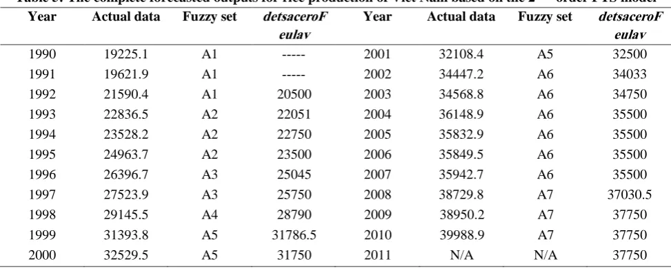
wh+ 𝛾−1 ; with ( 1 ≤ i ≤ 𝛾) (8) From forecasted rules above and based on Table 4, we complete forecasted results rice production of Viet Nam the period from 1990 to 2011 based on 2nd-order FTS model with seven intervals are listed in Table 5.
Table 5: The complete forecasted outputs for rice production of Viet Nam based on the 2nd– order FTS model
Year Actual data Fuzzy set detsaceroF
eulav
Year Actual data Fuzzy set detsaceroF
eulav
1990 19225.1 A1 --- 2001 32108.4 A5 32500
1991 19621.9 A1 --- 2002 34447.2 A6 34033
1992 21590.4 A1 20500 2003 34568.8 A6 34750
1993 22836.5 A2 22051 2004 36148.9 A6 35500
1994 23528.2 A2 22750 2005 35832.9 A6 35500
1995 24963.7 A2 23500 2006 35849.5 A6 35500
1996 26396.7 A3 25045 2007 35942.7 A6 35500
1997 27523.9 A3 25750 2008 38729.8 A7 37030.5
1998 29145.5 A4 28790 2009 38950.2 A7 37750
1999 31393.8 A5 31786.5 2010 39988.9 A7 37750
2000 32529.5 A5 31750 2011 N/A N/A 37750
The performance of proposed model can be assessed by comparing the difference between the forecasted values and the actual values. The widely used indicators in time series models comparisons are the root mean square error (RMSE) according to (9) as follows:
R𝑀𝑆𝐸 = 1
𝑛 (𝐹𝑡− 𝑅𝑡) 2 𝑛
𝑡=γ (9)
Where, Rt denotes actual value at year t, Ft is forecasted value at year t, n is number of the forecasted data, γ is
order of the fuzzy logical relationships
B. Forecasting model based on combined the high – order FTS and PSO algorithm
To improve forecasted accuracy of the proposed, the effective lengths of intervals and fuzzy logical relationship groups which are two main issues presented in this paper. A novel method for forecasting rice production is developed by PSO algorithm to adjust the length each of intervals in the universe of discourse without increasing the number of intervals
ISSN(E): 2277-128X, ISSN(P): 2277-6451, pp. 75-84
Algorithm 2: The FTS-PSO algorithm
1.Initialize all particles‟ positions Xid , velocities Vid and parameters of the proposed method. These parameters are:
Number of particles is 50
Maximum number of iterations is 100
The value of inertial weigh ω be linearly decreased from 𝜔𝑚𝑎𝑥 = 0.9 to𝜔𝑚𝑖𝑛 = 0.4
The coefficient C1 equal C2 as 2
The position of particle id be limited by: 𝑥𝑚𝑖𝑛 + 𝑅𝑎𝑛𝑑 ∗ (𝑥𝑚𝑎𝑥 − 𝑥𝑚𝑖𝑛) ; where 𝑥𝑚𝑖𝑛 𝑎𝑛𝑑 𝑥𝑚𝑎𝑥 are lower and upper bounds of universal set, respectively.
The velocity of particle id be exceeded by 𝑣𝑚𝑖𝑛 + 𝑅𝑎𝑛𝑑 ∗ (𝑣𝑚𝑎𝑥 − 𝑣𝑚𝑖𝑛)
2.While the stop condition (maximum iterations or minimum RMSE criteria) is not satisfied do
2.1. For particle id, (1≤ 𝑖𝑑 ≤ N) do
Define linguistic values according to all
intervals defined by the current position of particle id
Fuzzify all historical data by Step 4 in Subsection 3.1
Create all 𝛾 − order fuzzy relationships by Step 5 in Subsection 3.1
Make all 𝛾 − order fuzzy relationship groups by Step 6 in Subsection 3.1
Calculate forecasting values by Step 7 in Subsection 3.1
Compute the RMSE values for particle id based on Eq. (9)
Update the personal best position of particle id according to the RMSE values mentioned above.
end for
2.2. Update the global best position of all particles according to the RMSE values mentioned above.
3.For particle i, (1≤ 𝑖𝑑 ≤ N) do
move particle id to another position according to (1) and (2)
end for
update 𝜔 according to Eq. (3)
end while
IV. EXPERIMENTAL RESULTS
In this paper, we apply the proposed model to forecast the rice production of Viet Nam with the whole historical data the period from 1990 to 2010 is listed in Table 1 and we also the proposed model to handle other forecasting problems, such as the empirical data for the enrolments of University of Alabama [4] from 1971 to 1992 are used to perform comparative study in the training phase.
A. Experimental results for forecasting rice production of Viet Nam
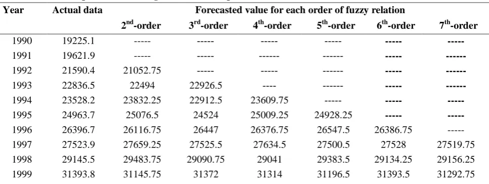
In this section, we apply the proposed method for forecasting the rice production from 1990 to 2010 are listed in Table 1. Our proposed model is executed 20 runs for each order, and the best result of runs at each order is taken to be the final result. During simulation with parameters are expressed in algorithm 2, the number of intervals is kept fix for the proposed model. The forecasted accuracy of the proposed method is estimated using the RMSE value (9). The forecasted results of proposed model under number of interval as 14 and various orders are listed in Table 6.
Table 6: The completed forecasting results for rice production data of Viet Nam under deferent orders of FTS
Year Actual data Forecasted value for each order of fuzzy relation
2nd-order 3rd-order 4th-order 5th-order 6th-order 7th-order
1990 19225.1 --- --- --- --- --- ---
1991 19621.9 --- --- --- --- --- ---
1992 21590.4 21052.75 --- --- --- --- ---
1993 22836.5 22494 22926.5 ---- --- --- ---
1994 23528.2 23832.25 22912.5 23609.75 --- --- ---
1995 24963.7 25076.5 24524 25009.25 24928.25 --- ---
1996 26396.7 26116.75 26447 26376.75 26547.5 26386.75 ---
1997 27523.9 27659.25 27525.5 27634.5 27500.5 27528 27519.75
1998 29145.5 29483.75 29090.75 29041 29383.5 29134.25 29156.25
ISSN(E): 2277-128X, ISSN(P): 2277-6451, pp. 75-84
2000 32529.5 32202.25 32298.25 32360.75 32404.5 32332 32351.5
2001 32108.4 32199.25 32295.25 32346.75 32387.5 32322 32347
2002 34447.2 34855 34334.25 34429 34522.25 34515.75 34495.25
2003 34568.8 34832 34330.25 34422.5 34518.75 34510.75 34489.25
2004 36148.9 35834 35720.75 36023.25 35999.25 35945.75 35981.75
2005 35832.9 35834 35692.25 35998.25 35975.25 35921.25 35955.25
2006 35849.5 35834 35692.25 35998.25 35975.25 35921.25 35955.25
2007 35942.7 35834 36283.6 35998.25 35975.25 35921.25 35955.25
2008 38729.8 38061 38161.6 38805.25 38805.25 38848.25 38833.75
2009 38950.2 39046 38745.5 38795.75 38793.25 38836.25 38826.75
2010 39988.9 39046 39617 39807.75 39959.5 39967 39955
2011 N/A 39046 39572.8 39680.9 39749.9 39687.85 39613.15
RMSE 369.34 297.37 127.5 139.75 108.05 116.2
From Table 6, it can be seen that the performance of the proposed model is improved a lot with increasing number of orders in the same number of interval. Particularly, the proposed model gets the lowest RMSE value of 108.05 with 6th-order fuzzy logical relationship.
B. Experimental results for forecasting enrolments
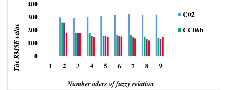
In order to verify the forecasting effectiveness of the proposed model under different number of orders and kept number of intervals of 7 , three FTS models in, C02[6] and CC06[9]and HPSO[17], are examined and compared. The forecasted accuracy of the proposed method is estimated by using the RMSE function (9). From the parameters are expressed in Algorithm 2. Our proposed model is executed 20 runs, and the best result of runs is taken to be the final result. A comparison of the forecasting accuracy of all models mentioned above and the proposed model, are listed in Table 7. where all models use the high-order FTS to forecast enrolments of university of Alabama in the training phase.
Table 7: A comparison of the RMSE value between our model and C02 model, CC06b model, HPSO model under different number of orders and the number of interval is 7.
Models Number of order of fuzzy relations
2 3 4 5 6 7 8 9
C
02 298.48 294.44 298.96 307.47 313.39 322.59 319.65 320.6
CC 06
b 260.45 176.42 178.91 158.06 164.26 164.22 149.63 136.87
OSPH 259.08 177.89 152.55 153.41 153.85 143.7 130.79 134.06
Our model 178.24 177.09 145.63 146.85 149.56 136.09 121.61 144.52
From Table 7, it can be seen that the accuracy of the proposed model is improved significantly. Particularly, our model gets the lower RMSE values than three models presented in C02 [6] and CC06 [9]and HPSO [17]. These finding suggest that the proposed model is able to provide effective forecasting capability for the high – order FTS model with different number of orders in the same number of interval is 7.
To be clearly visualized. From Fig.1, the graphical comparison clearly shows that the forecasting accuracy of the proposed model is more precise than those of existing models with the different number of orders.
Fig. 1. A comparison of the MSE values for 7 intervals with different high-order fuzzy relationships.
0 100 200 300 400
1 2 3 4 5 6 7 8 9
T
h
e
R
MS
E
v
a
lu
e
Number oders of fuzzy relation
C02
ISSN(E): 2277-128X, ISSN(P): 2277-6451, pp. 75-84
V. CONCLUSIONS
In this paper, a new hybrid forecasting model based on combined FTS and PSO is presented to improve forecasting. First, the proposed model is implemented for forecasting of rice production of Viet Nam. Subsequently, we proved correctness and robustness of the proposed model by testing and verifying it on historical enrolments data and comparing with those of existing models in the training phase. The main contributions of this paper are illustrated in the following. First, the author shows that the forecasted accuracy of the fuzzy forecast model can be improved by considering more information of latest fuzzy fluctuation within all current states of all fuzzy relationships. Second, the PSO algorithm for the optimized lengths of intervals is developed to adjust the interval lengths by searching the space of the universe. Third, based on the performance comparison in Tables 7 and Fig 1 the author shows the proposed model outperforms previous forecasting models for the training phase with various orders in this domain. Although this stud y shows the superior forecasting capability compared with the existing forecasting models, but the proposed model is only tested by two problems: enrolments data and rice production dataset based on one factor FTS. To continue considering the effectiveness of the fore-casting model in the future, the proposed model can be extended to deal with multidimensional time series data such as: Stock market prediction, weather forecast, traffic accidentprediction and so on.
REFERENCES
[1] Q. Song and B. S. Chissom, Fuzzy time series and its models, Fuzzy Sets and Systems, vol.54, no.3,(1993a) 269-277.
[2] Q. Song and B. S. Chissom, Forecasting enrolments with fuzzy time series - Part I, Fuzzy Sets and Systems, vol.54, no.1, (1993b) 1-9.
[3] Q. Song and B. S. Chissom, Forecasting enrolments with fuzzy time series - part II, Fuzzy Sets and System, vol. 62, (1994) 1-8.
[4] S.M. Chen, “Forecasting Enrolments based on Fuzzy Time Series,” Fuzzy set and systems, vol. 81, (1996) 311-319.
[5] K. Huarng, Effective lengths of intervals to improve forecasting in fuzzy time series, Fuzzy Sets and Systems, vol.123, no.3, (2001b) 387-394.
[6] S. M. Chen, Forecasting enrolments based on high-order fuzzy time series, Cybernetics and Systems, vol.33, no.1, (2002) 1-16.
[7] H. K. Yu, A refined fuzzy time-series model for forecasting, Physical A: Statistical Mechanics and Its Applications, vol.346, no.3-4, (2005) 657-681.
[8] Chen, S.-M., & Chung, N.-Y. Forecasting enrollments using high-order fuzzy time series and genetic algorithms: Research Articles. International Journal of Intelligent Systems, 21, (2006a) 485–501.
[9] Chen, S.-M., & Chung, N.-Y. Forecasting enrollments of students by using fuzzy time series and genetic algorithms. International Journal of Intelligent Systems, 17, (2006b) 1–17.
[10] Singh, S. R. A simple method of forecasting based on fuzzy time series. Applied Mathematics and Computation, 186, (2007a) 330–339.
[11] Singh, S. R.. A simple method of forecasting based on fuzzy time series. Applied Mathematics and Computation, 186, (2007b) 330–339.
[12] Chen, T.-L., Cheng, C.-H., & Teoh, H.-J., High-order fuzzy time-series based on multi-period adaptation model for forecasting stock markets. Physical A: Statistical Mechanics and its Applications, 387, (2008) 876–888. [13] Chu, H.-H., Chen, T.-L., Cheng, C.-H., & Huang, C.-C. . Fuzzy dual-factor time- series for stock index
forecasting. Expert Systems with Applications, 36, (2009) 165–171
[14] Lee, L.-W. Wang, L.-H., & Chen, S.-M, Temperature prediction and TAIFEX forecasting based on high order fuzzy logical relationship and genetic simulated annealing techniques, Expert Systems with Applications, 34, (2008b) 328–336.
[15] Ling-Yuan Hsu et al. Temperature prediction and TAIFEX forecasting based on fuzzy relationships and MTPSO techniques, Expert Syst. Appl.37, (2010) 2756–2770.
[16] L. A. Zadeh, 1965, Fuzzy sets, Information and Control, vol.8, no.3, pp.338-353.
[17] I. H. Kuo, et al., An improved method for forecasting enrolments based on fuzzy time series and particle swarm optimization, Expert systems with applications, 36 , (2009) 6108–6117.
[18] I-H. Kuo, S.-J. Horng, Y.-H. Chen, R.-S. Run, T.-W. Kao, R.-J. C., J.-L. Lai, T.-L. Lin, Forecasting TAIFEX based on fuzzy time series and particle swarm optimization, Expert Systems with Applications 2(37), (2010) 1494–1502.
ISSN(E): 2277-128X, ISSN(P): 2277-6451, pp. 75-84 [20] Ling-Yuan Hsu et al. Temperature prediction and TAIFEX forecasting based on fuzzy relationships and
MTPSO techniques, Expert Syst. Appl.37, (2010) 2756–2770.
[21] S. Pritpal, B. Bhogeswar, High-order fuzzy-neuro expert system for time series forecasting, Knowl.-Based Syst. 46 (2013) 12–21.
[22] L. Al - Mataneh, A. Senta, S.Bani –Ahmad, J.Alshaer and Al–oqily. Development of temperature based weather forecasting model using Neural network and fuzzy logic. 12 (2014) 343-366.