BAYESIAN IMAGE RESTORATION, USING CONFIGURATIONS
T
HORDISL
INDAT
HORARINSDOTTIRThe T.N. Thiele Centre, Department of Mathematical Sciences, University of Aarhus, Denmark. The MR Research Centre, Skejby University Hospital, University of Aarhus, Denmark.
e-mail: [email protected] (Accepted October 30, 2006)
ABSTRACT
In this paper, we develop a Bayesian procedure for removing noise from images that can be viewed as noisy realisations of random sets in the plane. The procedure utilises recent advances in configuration theory for noise free random sets, where the probabilities of observing the different boundary configurations are expressed in terms of the mean normal measure of the random set. These probabilities are used as prior probabilities in a Bayesian image restoration approach. Estimation of the remaining parameters in the model is outlined for salt and pepper noise. The inference in the model is discussed in detail for 3×3 and 5×5 configurations and examples of the performance of the procedure are given.
Keywords: Bayesian image analysis, configurations, digital image analysis, salt and pepper noise, stochastic geometry.
INTRODUCTION
The comparison of neighbouring grid points in a discrete realisation of a random closed set Z in
R2 has been used for decades to make inference on
various characteristics of the random set. A classical result, cf. Serra (1982), states that the information obtained by comparing pairs of neighbouring grid points can be used to estimate the mean length of the total projection of the boundary of the random set in directions associated with the digitisation. This, in turn, yields certain information about the directional properties of the boundary. Larger configurations, such as grid squares of size 2×2 or 3×3, were used in
Ohseret al.(1998) and Ohser and M¨ucklich (2000) to estimate the area density, length density, and density of the Euler number ofZ.
In Jensen and Kiderlen (2003) and Kiderlen and Jensen (2003), the authors use grid squares of size n×n,n≥2, to estimate the mean normal measure of
the random set Z. The knowledge of this can then be used to quantify the anisotropy of Z. Events of type tB⊂Z,tW ⊂R2\Z are observed, where tBandtW
are finite subsets of the scaled standard gridtZ2. The
probability of such events,
P(tB⊂Z,tW ⊂R2\Z),
can effectively be estimated by filtering the discrete image. In digitised images, B usually stands for “black” points and W for “white” points. Here, we use the notion point for the mid-point of a pixel in the digitised image. We will not distinguish between
a pixel and its mid-point and we use both notions in the following.
Another interesting aspect in the analysis of discrete planar random sets is the restoration of the random set from a noisy image. If the mean normal measure of the random set Z is known, the method in Kiderlen and Jensen (2003) and Jensen and Kiderlen (2003) can be reversed to obtain the prior probabilities for a Bayesian restoration procedure. The fundaments for Bayesian image analysis were developed by Grenander (1981), while the method itself was developed and popularised mainly by Geman and Geman (1984). For further readings on the subject, seee.g.Chalmond (2003) and Winkler (2003).
Hartvig and Jensen (2000) introduce a spatial mixture modelling approach to the Bayesian image restoration. They consider n×n neighbourhoods
around each pixel in the image, where n ≥ 3
This is showed in Kiderlen and Jensen (2003) where, asymptotically, a black and white configuration has a positive prior probability if and only if there exists a line going through the centre of at least two pixels that separates the black and the white points and hits only points of one colour. We use this theory to specify new prior probabilities for the spatial mixture model of Hartvig and Jensen (2000).
PRELIMINARIES
A compact convex subset ofR2is called aconvex
bodyand we denote byK the family of convex bodies
in R2. Theconvex ring, denoted by R, is the family
of finite unions of convex bodies while the extended convex ringis the family of all closed subsetsF∈R2
such thatF∩K∈Rfor allK∈K. Further, we denote
byL(K,·) thenormal measure of K ∈R on the unit
circle S1. For a Borel set A∈B(S1), L(K,A) is the
length of the part of the boundary of K with outer normal inA.Lis thus a Borel measure on S1 and the total mass L(K,S1) is just the boundary length L(K)
ofK. The normal measure is sometimes called the first surface area measure and then denoted byS1(K,·),cf. Schneider (1993).
Now, letZ be a stationary random set inR2 with
values in the extended convex ring. We assume in the following thatZsatisfies the integrability condition
E2N(Z∩K)<+∞, (1)
for all K ∈K . Here, N(U) is the minimal number
k ∈N such thatU =∪ki
=1Ki with Ki ∈K ifU 6= /0 and N(/0) =0. This condition is stricter than most standard integrability conditions, but it guarantees that the realisations of Z do not become too complex in structure. The mean normal measure ofZ is defined by
¯
L(Z,·) = lim
r→+∞
EL(Z∩rK,·)
ν2(rK) ,
where ν2 is the Lebesgue measure on R2. See e.g.
Schneider and Weil (2000) for more details.
A digitisation (or discretisation) of Z is the intersection of Z with a scaled lattice. For a fixed scaling factort>0, we considerZ∩tL, where
L:=Z2={(i,j):i,j∈Z}
is the usual lattice of points with integer coordinates. The lattice square
Ln:=n(i,j):i,j=−n−1
2 , . . . , n−1
2 o
,
consists ofn2 points (n≥3,nodd). Here, we follow the notation in Hartvig and Jensen (2000) and place the lattice square around a centre pixel. As we only consider lattice squares with odd number of points, this should not cause any conflicts in the notation. A line passing through at least two points ofLnwill be called
ann-lattice line.
Let X ⊂tZ2 be a finite set and t >0. A binary
image onX is a function f :X → {0,1}. Here, f is
given by f(x) = {x∈Z∩X} so that f is a random function due to the randomness of the setZ. We call a certain pattern of the values of f on a n×n grid a
configuration. We denote it byCn
t, wheret >0 is the
resolution of the grid, as in the definition of a lattice above. The elements of the configuration are numbered to match the numbering of the elements in the lattice squareLn. Forn=3 this gives
Ct3=
c−1,1 c0,1 c1,1
c−1,0 c0,0 c1,0
c−1,−1 c0,−1 c1,−1
t
,
and similarly for other allowed values ofn. If the size of the configuration is clear from the context, we will omit the indexn. Examples of 3×3 configurations are
h• ◦ ◦
• ◦ ◦ • • ◦
i t
h• ◦ ◦
• ◦ • • • ◦
i t
h◦ • •
• ◦ • • • ◦
i t ,
where the sign•means that f(x) =1 or equivalently z∩ {x} 6= /0, while ◦ means that f(x) = 0 or equivalentlyz∩ {x}= /0. Here, z is the realisation of the random setZ observed in the image f.
CONFIGURATION PROBABILITIES
Let f :X → {0,1}be an image as before and letZ
be a stationary random set that fulfils Eq. 1. In Kiderlen and Jensen (2003), the authors show that forn>0, a
givenx∈X, and a given configurationCt,
lim t→0+
1
tP Z∩t(Ln+x) =Ct
=
Z
S1h(−v)L¯(Z,dv).
(2) The functionhis given by
h(·) = min
x∈Bhx,·i −maxx∈Whx,·i +
where (tB,tW) = Ct is the partitioning of the
configuration Ct in “black” and “white” points, that is, tB⊂Z and tW ⊂R2\Z. Here, g+:=max{g,0}
denotes the positive part of the functiong andhx,yi
denotes the usual inner product of the vectorsxandy. A configurationCt with non-identically zerohis called an informative configuration.Ct is informative if and only if there exists an-lattice line separatingtBandtW not hitting both of them. More precisely,Ct = (tB,tW)
is informative if and only if there exists ann-lattice line g such thattBis on one side ofg,tW is on the other side of g and all the lattice points on g are either all black or all white.
Furthermore, it is shown in Jensen and Kiderlen (2003) that for a given informative configuration Ct, there exist vectorsa,b∈R2such that
h(−v) =min{ha,vi+,hb,vi+},
for all v ∈S1. These results are then used to obtain
estimators for the mean normal measure ¯L(Z,·)based
on observed frequencies of the different types of configurations. If we, on the other hand, assume we have a discrete noisy image in R2, where the
underlying image is a realisation of a stationary random closed set Z with a known mean normal measureL(Z,·), Eq. 2 provides prior probabilities in
a Bayesian restoration procedure.
As an example, let us assume thatZ is isotropic. Then, the mean normal measure ¯L(Z,·) is, up to
a positive constant of proportionality, the Lebesgue measure on[0,2π). Eq. 2 thus becomes
lim t→0+
1
tP Z∩t(Ln+x) =Ct
=k
Z 2π
0 min
ha,y(θ)i+,hb,y(θ)i+ dθ, (3)
where y(θ) = (cosθ,sinθ) and k >0 is a constant.
For t >0 small enough, such that only informative,
all black, and all white configurations have positive probability, this gives the marginal probability of each informative configurations up to a constant of proportionality.
Forn=3, the vectorsaandbare given in Jensen and Kiderlen (2003). We can thus insert those values without further effort into the right hand side of Eq. 3. Forx∈X, this gives
P A=
p0, Ct=
h◦ ◦ ◦
◦ ◦ ◦ ◦ ◦ ◦
i t p1, Ct=
h• • •
• • • • • •
i t p2, Ct∈R
h• ◦ ◦
• ◦ ◦ • ◦ ◦
i t,
h• • ◦
• • ◦ • • ◦
i t
p3, Ct∈R
h◦ ◦ ◦
• ◦ ◦ • • ◦
i t,
h• ◦ ◦
• • ◦ • • •
i t
p4, Ct∈R
h• • ◦
• • • • • •
i t,
h◦ ◦ ◦
◦ ◦ ◦ • ◦ ◦
i t
p5, Ct∈R
h• ◦ ◦
• ◦ ◦ • • ◦
i t,
h• ◦ ◦
• • ◦ • • ◦
i t, h• • ◦
• • ◦ • • •
i t,
h◦ ◦ ◦
• ◦ ◦ • ◦ ◦
i t
0, otherwise,
where A is the event Z∩(tL3+x) =Ct and R(·) is
the set of all possible rotations and reflections. The probabilities p2, . . . ,p5 are determined from Eq. 3 up
to a multiplicative constantc. They are given by p2=c5sin(atan(2))−4,
p3=c5sin(atan(2))−3√2,
p4=c2−√2,
p5=c1+√2−52sin(atan(2)).
As the total probability is 1, we have
p0+p1+8(p2+p3+p4) +32p5=1.
We can thus expressc in terms of the other unknown probabilities,
c=1−p0−p1 16 .
For n=5, we have used the methods described in Jensen and Kiderlen (2003) to determine the informative 5×5 configurations and the vectorsaand
bfor each configuration. We have then calculated the prior probabilities in the same manner as described above for 3×3 configurations. The results from this can be found in Appendix A.
Knowledge of the mean normal measure of Z will not give us information about the probability of observing all white and all black configurations, as the mean normal measure is a property of the boundary of the set. The remaining parameters,p0andp1must thus be estimated from the data. This problem is treated in the next section.
RESTORATION OF A NOISY
IMAGE
LetF :X → {0,1}be a binary image on a finite
as a realisation of an isotropic stationary random setZ with noise. Note that the randomness in the imageF is two-fold. First, the noise free image is random due to the randomness of the setZ. Second, a random noise is added to the image. By Bayes rule we have, forx∈X
and a given configurationCt,
P Z∩(tLn+x) =Ct|F(tLn+x)
∝P Z∩(tLn+x) =Ct
×p F(tLn+x)|Z∩(tLn+x) =Ct.
We assume that F(xi) and F(xj) are conditionally independent given Z for all xi,xj ∈X, and that the
conditional distribution ofF(x)givenZ only depends onZ∩xfor allx∈X. Under these conditions, we get
p F(tLn+x)|Z∩(tLn+x) =Ct
= n2
∏
k=1p F(yk)|Z∩ {yk}={ck}
,
where{yk}nk=21=tLn+xand{ck}nk2=1=Ct.
By summing over the neighbouring states, we obtain the probability ofZhitting a single pointx∈X,
P Z∩ {x} 6=/0|F(tLn+x)
∝
∑
{Ct:c00=•}
P Z∩(tLn+x) =Ct
×
n2
∏
k=1p F(yk)|Z∩ {yk}={ck}
=:S1(x). (4)
The probability ofZ not hitting a single pointx∈X is
obtained in a similar way. It is given by
P Z∩ {x}=/0|F(tLn+x)
∝
∑
{Ct:c00=◦}
P Z∩(tLn+x) =Ct
×
n2
∏
k=1p F(yk)|Z∩ {yk}={ck}
=:S2(x). (5)
As the probabilities in Eq. 4) and Eq. 5 sum to one, we only need to compareS1(x)andS2(x)for determining the restored value of the image for a pixel x. The restored value is 1 ifS1(x)>S2(x)and 0 otherwise.
To compareS1(x)andS2(x), we need to determine the densities p F(x)|Z∩ {x}
which depend on the distribution of the noise. As an example, we consider salt and pepper noise. That is, a black point is replaced
by a white point with probability q, and vice versa. More precisely,
p F(x)|Z∩ {x}
=qF(x)(1−q)1−F(x)
Z∩ {x}=/0 + (1−q)F(x)q1−F(x)
Z∩ {x} 6=/0 ,
for some 0≤q≤1. This noise model has one unknown
parameter,q, which must be estimated from the data. Further, we need to determine the marginal probability P Z ∩(tLn+x) = Ct of observing a
given configuration, Ct. A method to obtain the prior probabilities of observing the different types of boundary configurations, that is configurations that contain both black and white points, is given in the previous section. We still lack information about the prior probabilities of observing configurations that are all black or all white, that is
p0=P
Z∩(tL3+x) =
h◦ ◦ ◦
◦ ◦ ◦ ◦ ◦ ◦
i t
and
p1=P
Z∩(tL3+x) =
h• • •
• • • • • •
i t
ifn=3 and similarly for largern.
We use the parameter estimation approach introduced in Hartvig and Jensen (2000) which is related to maximum likelihood estimation. Within the model, we can calculate the marginal density of an n×nneighbourhood. It is given by
p F(tLn+x);p0,p1,q
=
∑
Ct
p F(tLn+x)|Z∩(tLn+x) =Ct;q
×P Z∩(tLn+x) =Ct;p0,p1
=p0q∑F(yk)(1−q)n2−∑F(yk)
+p1qn2−∑F(yk)(1−q)∑F(yk)
+1−p0−p1 A(n) C
∑
tinform. h
B(Ct)
×
n2
∏
k=1qF(yk)(1−q)1−F(yk) {Z∩ {yk}= /0}
+q1−F(yk)(1−q)F(yk) {Z∩ {y
k} 6=/0} i
,
where the constantB(Ct)is given by the integral on the right hand side of Eq. 3 and A(n) =∑Ctinform.B(Ct). We haveA(3) =16 andA(5) =32.
A possibility for estimating the parameters p0,p1,
andqis to maximise the contrast function γ(p0,p1,q) =
∑
x∈X
This is, however, computationally a very demanding task. We have therefore used a simplified version of the approach. The probability that a single pointx∈X
is in the setZis
P Z∩ {x} 6= /0=
∑
{Ct:c00=•}
P Z∩(tLn+x) =Ct
=1−p0−p1 2 +p1 =1−p0+p1
2 ,
as exactly half of the boundary configurations have a black mid-point. The marginal density of a single point is thus given by
p F(x);p0,p1,q
=P Z∩ {x} 6=/0;p0,p1
p F(x)|Z∩ {x} 6= /0;q +P Z∩ {x}=/0;p0,p1p F(x)|Z∩ {x}=/0;q
=1 2 h
(1−p0+p1)q1−F(x)(1−q)F(x)
+ (1+p0−p1)qF(x)(1−q)1−F(x)i.
The corresponding contrast function
γm(p0,p1,q) =
∑
x∈Xlogp F
(x);p0,p1,q,
can easily be differentiated with repect to the parametersp0,p1, andq. The differentiation yields that the maximum ofγmis obtained when
p1=p0+2∑F(x)− |X| |X|(1−2q) ,
where |X| denotes the number of points in X. In
the examples in the following, we have inserted this into Eq. 6 and maximised γ on a grid with q ∈ [0.05,0.1, . . . ,0.45,0.49] and p0 ∈[0.05,0.1, . . . ,0.9]
under the constraints
2p0+2∑F(x)− |X|
|X|(1−2q) <1, p0+
2∑F(x)− |X| |X|(1−2q) ≥0.
EXAMPLES
We illustrate the method by applying it to two synthetic datasets and one real data set. We use the salt and pepper noise model and isotropic priors for the configuration probabilities in all three examples. The method can not be used directly to restore the values on the edge of an image. In the examples below, we have therefore a one-pixel-wide edge of white (background)
pixels in each restored image for n=3 and a two-pixel-wide edge of white pixels in each restored image for n=5. Another possibility here would be to add either a one-pixel-wide boundary of white pixels for n=3, or a two-pixel-wide boundary of white pixels for n=5, around the noisy image before restoration. This will, however, lead to a slight underestimate of black pixels on the edge. We will quantify the results by the classification error. The classification error is estimated as the percentage of misclassified pixels (either type I or type II errors). The results given for the classification error are based on those pixels from the interior of each image where there are no edge effects. Example 1 (Boolean model with isotropic grains). The first example is based on digitisation of a simulated Boolean model, see Schneider and Weil (2000). Boolean models are widely used as simple geometric models for random sets. The simulation of a Boolean model is a two-step procedure. First, independent uniform points are simulated in a sampling window. Second, a random grain is attached to each point. The grains are independent from one another and from the points. In order to avoid edge effects, the sampling window must be larger than the target window. Here, the target window is the unit square and the grains are circular discs with random radii. The radius of each grain is a uniform number from the interval [0.0375,0.15]. Fig. 1 (left) shows
a realisation of this model. We have then digitised the image with t =0.01 which gives a resolution of
100×100. The digitised image is shown in Fig. 1
(right).
Fig. 1. Boolean model with circular grains. Left: a realisation of the model on the unit square. Right: a digitised image of the realisation with resolution 100×100.
The digitised realisation of the Boolean model from Fig. 1 (right) is now our original image. We have added salt and pepper noise to it for three different values of the noise parameter q. The noisy images are shown in Fig. 2 (top row). In the leftmost image we have q = 0.25, in the middle image q = 0.33,
and in the rightmost imageq=0.4. We have restored
the original image from the noisy images using both 3×3 configurations and 5×5 configurations
as described in the previous section. The resulting images for 3×3 configurations are shown in the
configurations are shown in the bottom row of Fig. 2. The parameter estimates and the classification errors for the restoration are given in Table 1.
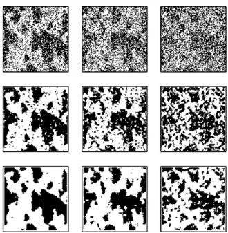
Fig. 2. Restoration of the digitised realisation of the Boolean model with isotropic grains. Top row: the original image disturbed with salt and pepper noise for q equal to0.25,0.33,and0.4. Middle row: estimates of
the true image using3×3configurations. Bottom row:
estimates of the true image using5×5configurations.
Example 2 (Boolean model with non-isotropic
grains). The grains in the Boolean model are here
the right half of circular discs with random radii. The radius of each grain is a uniform number from the interval[0.0375,0.15] and the target window is again
the unit square. A realisation of this model is shown in Fig. 3 (left). As before, we have digitised the image witht =0.01 which gives a resolution of 100×100.
The digitised image is shown in Fig. 3 (right).
Fig. 3.Boolean model with non-isotropic grains. Left: a realisation of the model on the unit square. Right: a digitised image of the realisation with resolution 100×100.
We have proceeded exactly as in the previous example. The noisy images are shown in Fig. 4 (top row). In the leftmost image we have q = 0.25, in
the middle image q=0.33, and in rightmost image
q=0.4. The restored images for 3×3 configurations
are shown in the middle row of Fig. 4 and the restored
images for 5×5 configurations are shown in the
bottom row of Fig. 4. Further, Table 2 shows the parameter estimates and the classification errors for the restoration.
Fig. 4.Restoration of the digitised realisation of the non-isotropic Boolean model. Top row: the original image disturbed with salt and pepper noise for q equal to 0.25,0.33, and 0.4. Middle row: estimates of the
true image using 3×3 configurations. Bottom row:
estimates of the true image using5×5configurations.
Example 3 (Image from steel data). Our last
example is an image showing the micro-structure of steel. The image is from Ohser and M¨ucklich (2000), where it has been analysed to estimate the mean normal measure, see also Jensen and Kiderlen (2003). The thresholded, binary image of the data is shown in Fig. 5. We have used Otsu’s method for the thresholding. This method minimises the intraclass variance of the black and the white pixels, see Otsu (1979). The resolution of the image is 896×1280
pixels.
Table 1.Parameter estimates, true parameter values, and classification errors for the restoration of a Boolean model with isotropic grains. The parameter estimates are based on five independent simulations of the degraded image. The standard errors of the estimates are given in parentheses. The classification errors are given in percentage.
n×n q qˆ p0 p0ˆ p1 p1ˆ Class. error
3×3 0.25 0.25(0) 0.30 0.31(0.02) 0.45 0.45(0.01) 8.98(0.55)
5×5 0.25 0.25(0) 0.20 0.21(0.02) 0.35 0.35(0.01) 5.11(0.39)
3×3 0.33 0.32(0.03) 0.30 0.33(0.08) 0.45 0.48(0.10) 17.79(0.01)
5×5 0.33 0.33(0.03) 0.20 0.22(0.07) 0.35 0.37(0.09) 10.61(0.32)
3×3 0.40 0.40(0) 0.30 0.31(0.08) 0.45 0.45(0.06) 29.19(0.77)
5×5 0.40 0.40(0) 0.20 0.22(0.06) 0.35 0.36(0.05) 21.20(1.02)
Table 2.Parameter estimates, the true parameter values, and classification errors for the restoration of the non-isotropic Boolean model. The parameter estimates are based on five independent simulations of the degraded image. The standard errors of the estimates are given in parentheses. The classification errors are given in percentage.
n×n q qˆ p0 p0ˆ p1 p1ˆ Class. error
3×3 0.25 0.25(0) 0.48 0.47(0.03) 0.31 0.30(0.03) 9.03(0.15)
5×5 0.25 0.25(0) 0.39 0.39(0.02) 0.22 0.22(0.01) 5.05(0.29)
3×3 0.33 0.35(0) 0.48 0.55(0) 0.31 0.36(0.02) 18.27(0.88)
5×5 0.33 0.35(0) 0.39 0.44(0.02) 0.22 0.25(0.03) 10.72(0.60)
3×3 0.40 0.40(0) 0.48 0.48(0.03) 0.31 0.35(0.04) 29.06(0.52)
5×5 0.40 0.40(0) 0.39 0.36(0.04) 0.22 0.23(0.04) 20.62(0.74)
Fig. 6.Restoration of the steel data image. Left column: the original binary image disturbed with salt and pepper noise for q=0.25(upper image) and q=0.33(lower image). Middle column: estimates of the true image using
3×3configurations. Right column: estimates of the true image using5×5configurations.
We have added salt and pepper noise to the binary image for q=0.25 and q=0.33. The noisy images
are shown in Fig. 6 (left column). We have used the method described in the previous section for the restoration of the noisy images, using isotropic
priors for the informative configurations. The resulting images can be seen in Fig. 6 (middle column) for 3×3
configurations and in Fig. 6 (right column) for 5×5
Table 3.Parameter estimates, the true parameter values, and classification errors for the restoration of the steel data image. The parameter estimates are based on five independent simulations of the degraded image. The standard errors of the estimates are given in parentheses. The classification errors are given in percentage.
n×n q qˆ p0 p0ˆ p1 p1ˆ Class. error
3×3 0.25 0.25(0) 0.34 0.35(0) 0.45 0.46(0.002) 8.92(0.03)
5×5 0.25 0.25(0) 0.25 0.25(0) 0.35 0.36(0.002) 4.90(0.03)
3×3 0.33 0.35(0) 0.34 0.40(0) 0.45 0.53(0.003) 17.74(0.03)
5×5 0.33 0.35(0) 0.25 0.30(0) 0.35 0.43(0.003) 10.71(0.05)
COMPARISON WITH OTHER
METHODS
Other models for this type of Bayesian image restoration include Markov random field models. In Besag (1986), the author presented an iterative method for this type of image restoration where the local characteristics of the underlying true image are represented by a non-degenerate Markov random field. The author calls his method iterated conditional modes (ICM). As the name of the method indicates, the estimation under the model is performed iteratively where the possible parameters of the model and the reconstructed point pattern are updated in turn. This method is very flexible, though computationally quite intensive and depends on a smoothing parameter that cannot be directly estimated from the data. An extenstion of this method is the maximum a posteriori (MAP) method proposed in Greig et al.(1989). The MAP method is a special case of the ICM method where the estimated image is given by the image which maximises the posterior density. In this case there exists and efficient algorithm to calculate the estimate. There is though still the problem of a smoothness parameter that cannot be directly estimated from data. Further discussion of models of this type can be found in Chalmond (2003) and Winkler (2003).
In Hartvig and Jensen (2000), the authors proposed three prior models of different complexity for a similar type of restoration method as is described in this paper. These models also reflect the idea, that pixels of one colour tend to cluster rather than appear as single isolated voxels. They, however, do not take the actual spatial pattern of the neighbourhood into account.
In order to compare the method presented here to the methods mentioned above, we have used our method to reconstruct noisy versions of the image of an ”A” by Greiget al.(1989), see Fig. 7(a). The same image was used in Greiget al.(1989) and Hartvig and Jensen (2000) to show the performance of the methods mentioned above.
Fig. 7.The64×64binary image of an ”A” by Greig
et al. (1989) (a), the same image corrupted with salt and pepper noise with parameter q=0.25 (b), the
estimated true image using the method described in this paper with n=3 (c), and the estimate using the same method, but with n=5(d).
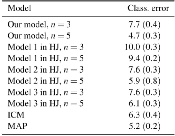
Table 4. Estimated classification errors for the models described above based on five independent reconstructions of noisy versions of the image in Fig. 7 (a). The results are given in percentage, standard errors are given in parentheses. The different models presented in Hartvig and Jensen (2000) (denoted HJ in the table) are denoted as in the orignal paper. All results except for the model presented in this paper are reproduced from Hartvig and Jensen (2000) and Greig et al. (1989).
Model Class. error
Our model,n=3 7.7(0.4)
Our model,n=5 4.7(0.3)
Model 1 in HJ,n=3 10.0(0.3)
Model 1 in HJ,n=5 9.4(0.2)
Model 2 in HJ,n=3 7.6(0.3)
Model 2 in HJ,n=5 5.9(0.8)
Model 3 in HJ,n=3 7.6(0.3)
Model 3 in HJ,n=5 6.1(0.3)
ICM 6.3(0.4)
MAP 5.2(0.2)
In Fig. 7, estimates under our method with noise parameter q = 0.25 are shown. This is the same
amount of noise as was used in the other papers. For comparability, we have added a two-pixel-wide boundary of black pixels to the image before adding the noise. This way, we can restore the whole original image using both 3×3 and 5×5 configurations. The
repetitions of the procedure is given in Table 4. For comparison, we have also reproduced the results on this image from Greiget al. (1989) and Hartvig and Jensen (2000). In the case of the ICM and the MAP methods, we only show the classification error for the value of the unknown smoothing parameter which gave the best results.
DISCUSSION
In the two first examples we have images of a similar type, the only difference is the mean normal measure of the boundary of the objects. In Example 1, the grains have isotropic boundaries which means that the model is using the correct prior probabilities for the configurations. In Example 2, on the other hand, there are some configurations that have much higher probability than suggested in the prior. The configurations
h◦ • •
◦ • • ◦ • •
i t and
h◦ ◦ •
◦ ◦ • ◦ ◦ •
i t
are, for instance, more likely to occur in the image than the configurations
h◦ ◦ ◦
• • • • • •
i t and
h◦ ◦ ◦
◦ ◦ ◦ • • •
i t.
According to the isotropic prior, however, these configurations are all equaly likely to occur. If we compare the results in Table 1 and Table 2, we see that the classification error in Example 2 is very similar to the classification error in Example 1 for the same amount of noise and the same type of model. This suggests that it is not necessary to know the mean normal measure of the boundary of the object precisely for our model to perform in a close to optimal way. Further, it can be seen from Table 4 that our method performs better or equally good as other similar methods, even though the ”random” set in the image in Fig. 7 is far from being isotropic which is assumed in the prior.
It is also clear from the results in Table 1-4 that the model using 5×5 configurations is superior
to the model using 3×3 configurations for all our
examples. This is not surprising since the true images are quite regular with large patches of either black or white pixels. One might suspect that the model using 3×3 configurations would be more appropriate
for images where the object Z consists of relatively small, disconnected components as in the example of simulated fMRI data in Hartvig and Jensen (2000). In this example, the 3×3 configurations give better
results than the 5×5 configurations for all three prior
models discussed in the paper. In our prior model, only informative configurations have a positive probability. That is, a boundary configuration has a positive prior probability if and only if there exists a line going through the centre of at least two pixels that separates the black and the white points and hits only points of one colour. If, however, the components ofZare very small compared to the resolution of the image, only very few boundary configurations will be of this type for large configurations. We would therefore expect similar results as in Hartvig and Jensen (2000).
Another consideration is whether it is of interest to consider larger configurations than 5×5
configurations. As one can see from Appendix A, the model is already quite complicated if we use 5×5 configurations. We think, therefore, that it
is computationally not feasible to consider larger configurations. Further, and maybe more importantly, very large configurations will tend to remove any finer details in the original image.
ACKNOWLEDGEMENTS
The author would like to thank Eva B. Vedel Jensen and Markus Kiderlen for many fruitful discussions and useful suggestions. Also, many thanks to Lars Madsen for the help with some of the technical issues.
REFERENCES
Besag J (1986). On the statistical analysis of dirty pictures. J Roy Statist Soc Ser B 48(3):259-302.
Chalmond B (2003). Modeling and inverse problems in image analysis. New York: Springer.
Geman S, Geman D (1984). Stochastic relaxation, Gibbs distributions, and the Bayesian restoration of images. IEEE Trans Pattern Anal 6:721-41.
Greig D, Porteous B, Seheult A (1989). Exact maximum a posteriori estimation for binary images. J Roy Statist Soc Ser B 51:271-9.
Grenander U (1981). Lectures in pattern theory Vol. I–III. New York: Springer.
Hartvig NV, Jensen JL (2000). Spatial mixture modeling of fMRI data. Hum Brain Mapp 11:233-48.
Jensen EBV, Kiderlen M (2003). Directional analysis of digitized planar sets by configuration counts. J Microsc 212:158-68.
Kiderlen M, Jensen EBV (2003). Estimation of the directional measure of planar random sets by digitization. Adv Appl Probab 35:583-602.
Ohser J, M¨ucklich F (2000). Statistical analysis of microstructures in material science. Chichester: John Wiley.
Ohser J, Steinbach B, Lang C (1998). Efficient texture analysis of binary images. J Microsc 192:20-8.
Otsu N (1979). A threshold selection method from gray-level histograms. IEEE Trans Syst Man Cyb 9:62-6. Schneider R (1993). Convex bodies: the Brunn-Minkowski
theory. Cambridge: Cambridge University Press. Schneider R, Weil W (2000). Stochastische Geometrie.
Stuttgart: Teubner, pp 214-8.
Serra J (1982). Image analysis and mathematical morphology. London: Academic Press.
Winkler G (2003). Image analysis, random fields and Markov chain Monte Carlo methods. 2nd edition. Berlin: Springer.
Woolrich MW, Behrens TEJ, Beckmann CF, Smith SM (2005). Mixture models with adaptive spatial regularization for segmentation with an application to fMRI data. IEEE Trans Med Imaging 24:1-11.
APPENDIX A
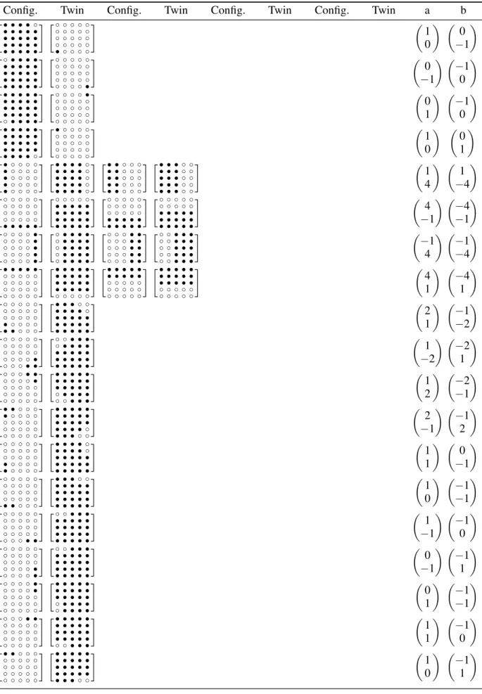
Using the methods described in Jensen and Kiderlen (2003), we have constructed all informative 5×5 configurations and calculated the vectors a and
b which are needed for the calculation of the prior probabilities of the informative configurations. The results are given in Table 5. We have omitted both the index for the resolution of the grid and the index for the size of the configuration to save space in the table.
In the examples presented above, we have used an isotropic prior for the boundary configurations. For x∈X, the prior probabilities for 5×5 configurations
are in this case given by
P A=
p0, Ct =
◦ ◦ ◦ ◦ ◦
◦ ◦ ◦ ◦ ◦ ◦ ◦ ◦ ◦ ◦ ◦ ◦ ◦ ◦ ◦ ◦ ◦ ◦ ◦ ◦
t
p1, Ct =
• • • • •
• • • • • • • • • • • • • • • • • • • •
t 0.5858c, Ct in group nr. 1, . . . ,4
0.2462c, Ct in group nr. 5, . . . ,8
0.2295c, Ct in group nr. 9, . . . ,12
0.1781c, Ct in group nr. 13, . . . ,20
0.1400c, Ct in group nr. 21, . . . ,24
0.1044c, Ct in group nr. 25, . . . ,32
0.1005c, Ct in group nr. 33, . . . ,36
0.0738c, Ct in group nr. 37, . . . ,44
0.0596c, Ct in group nr. 45, . . . ,52
0.0447c, Ct in group nr. 53, . . . ,60
0.0392c, Ct in group nr. 61, . . . ,68
0.0346c, Ct in group nr. 69, . . . ,76
0.0250c, Ct in group nr. 77, . . . ,84
0.0198c, Ct in group nr. 85, . . . ,92
0, otherwise.
Here, A is the event Z∩(tL5+x) =Ct. The prior
probabilities for the informative configurations have been calculated up to a multiplicative constant c by inserting the vectorsa andbin Table 5 into the right hand side of Eq. 3. The unknown constant c can be expressed in terms ofp0andp1by
Table 5.The 92 groups of informative 5 x 5 configurations.
No. Config. Twin Config. Twin Config. Twin Config. Twin a b
1
• • • • ◦
• • • • • • • • • • • • • • • • • • • •
◦ ◦ ◦ ◦ ◦ ◦ ◦ ◦ ◦ ◦ ◦ ◦ ◦ ◦ ◦ ◦ ◦ ◦ ◦ ◦ • ◦ ◦ ◦ ◦
1 0
0
−1
2
◦ • • • •
• • • • • • • • • • • • • • • • • • • •
◦ ◦ ◦ ◦ ◦ ◦ ◦ ◦ ◦ ◦ ◦ ◦ ◦ ◦ ◦ ◦ ◦ ◦ ◦ ◦ ◦ ◦ ◦ ◦ •
0
−1 −
1 0
3
• • • • •
• • • • • • • • • • • • • • • ◦ • • • •
◦ ◦ ◦ ◦ • ◦ ◦ ◦ ◦ ◦ ◦ ◦ ◦ ◦ ◦ ◦ ◦ ◦ ◦ ◦ ◦ ◦ ◦ ◦ ◦
0 1
−1
0
4
• • • • •
• • • • • • • • • • • • • • • • • • • ◦
• ◦ ◦ ◦ ◦ ◦ ◦ ◦ ◦ ◦ ◦ ◦ ◦ ◦ ◦ ◦ ◦ ◦ ◦ ◦ ◦ ◦ ◦ ◦ ◦
1 0
0 1
5
• ◦ ◦ ◦ ◦
• ◦ ◦ ◦ ◦ • ◦ ◦ ◦ ◦ • ◦ ◦ ◦ ◦ • ◦ ◦ ◦ ◦
• • • • ◦ • • • • ◦ • • • • ◦ • • • • ◦ • • • • ◦
• • ◦ ◦ ◦ • • ◦ ◦ ◦ • • ◦ ◦ ◦ • • ◦ ◦ ◦ • • ◦ ◦ ◦
• • • ◦ ◦ • • • ◦ ◦ • • • ◦ ◦ • • • ◦ ◦ • • • ◦ ◦
1 4
1
−4
6
◦ ◦ ◦ ◦ ◦
◦ ◦ ◦ ◦ ◦ ◦ ◦ ◦ ◦ ◦ ◦ ◦ ◦ ◦ ◦ • • • • •
◦ ◦ ◦ ◦ ◦ • • • • • • • • • • • • • • • • • • • •
◦ ◦ ◦ ◦ ◦ ◦ ◦ ◦ ◦ ◦ ◦ ◦ ◦ ◦ ◦ • • • • • • • • • •
◦ ◦ ◦ ◦ ◦ ◦ ◦ ◦ ◦ ◦ • • • • • • • • • • • • • • •
4
−1 −
4
−1
7
◦ ◦ ◦ ◦ •
◦ ◦ ◦ ◦ • ◦ ◦ ◦ ◦ • ◦ ◦ ◦ ◦ • ◦ ◦ ◦ ◦ •
◦ • • • • ◦ • • • • ◦ • • • • ◦ • • • • ◦ • • • •
◦ ◦ ◦ • • ◦ ◦ ◦ • • ◦ ◦ ◦ • • ◦ ◦ ◦ • • ◦ ◦ ◦ • •
◦ ◦ • • • ◦ ◦ • • • ◦ ◦ • • • ◦ ◦ • • • ◦ ◦ • • •
−1
4 −−14
8
• • • • •
◦ ◦ ◦ ◦ ◦ ◦ ◦ ◦ ◦ ◦ ◦ ◦ ◦ ◦ ◦ ◦ ◦ ◦ ◦ ◦
• • • • • • • • • • • • • • • • • • • • ◦ ◦ ◦ ◦ ◦
• • • • • • • • • • ◦ ◦ ◦ ◦ ◦ ◦ ◦ ◦ ◦ ◦ ◦ ◦ ◦ ◦ ◦
• • • • • • • • • • • • • • • ◦ ◦ ◦ ◦ ◦ ◦ ◦ ◦ ◦ ◦
4 1
−4 1
9
◦ ◦ ◦ ◦ ◦
◦ ◦ ◦ ◦ ◦ ◦ ◦ ◦ ◦ ◦ • ◦ ◦ ◦ ◦ • • ◦ ◦ ◦
• • • ◦ ◦ • • • • ◦ • • • • • • • • • • • • • • •
2 1
−1 −2
10
◦ ◦ ◦ ◦ ◦
◦ ◦ ◦ ◦ ◦ ◦ ◦ ◦ ◦ ◦ ◦ ◦ ◦ ◦ • ◦ ◦ ◦ • •
◦ ◦ • • • ◦ • • • • • • • • • • • • • • • • • • •
1
−2 −12
11
◦ ◦ ◦ • •
◦ ◦ ◦ ◦ • ◦ ◦ ◦ ◦ ◦ ◦ ◦ ◦ ◦ ◦ ◦ ◦ ◦ ◦ ◦
• • • • • • • • • • • • • • • ◦ • • • • ◦ ◦ • • •
1 2
−2
−1
12
• • ◦ ◦ ◦
• ◦ ◦ ◦ ◦ ◦ ◦ ◦ ◦ ◦ ◦ ◦ ◦ ◦ ◦ ◦ ◦ ◦ ◦ ◦
• • • • • • • • • • • • • • • • • • • ◦ • • • ◦ ◦
2
−1 −
1 2
13
◦ ◦ ◦ ◦ ◦
◦ ◦ ◦ ◦ ◦ ◦ ◦ ◦ ◦ ◦ • ◦ ◦ ◦ ◦ • ◦ ◦ ◦ ◦
• • • • ◦ • • • • ◦ • • • • • • • • • • • • • • •
1 1
0
−1
14
◦ ◦ ◦ ◦ ◦
◦ ◦ ◦ ◦ ◦ ◦ ◦ ◦ ◦ ◦ ◦ ◦ ◦ ◦ ◦ • • ◦ ◦ ◦
• • • ◦ ◦ • • • • • • • • • • • • • • • • • • • •
1 0
−1
−1
15
◦ ◦ ◦ ◦ ◦
◦ ◦ ◦ ◦ ◦ ◦ ◦ ◦ ◦ ◦ ◦ ◦ ◦ ◦ ◦ ◦ ◦ ◦ • •
◦ ◦ • • • • • • • • • • • • • • • • • • • • • • •
1
−1 −
1 0
16
◦ ◦ ◦ ◦ ◦
◦ ◦ ◦ ◦ ◦ ◦ ◦ ◦ ◦ ◦ ◦ ◦ ◦ ◦ • ◦ ◦ ◦ ◦ •
◦ ◦ • • • • • • • • • • • • • • • • • • • • • • •
0
−1 −
1 1
17
◦ ◦ ◦ ◦ •
◦ ◦ ◦ ◦ • ◦ ◦ ◦ ◦ ◦ ◦ ◦ ◦ ◦ ◦ ◦ ◦ ◦ ◦ ◦
• • • • • • • • • • • • • • • ◦ • • • • ◦ • • • •
0 1
−1 −1
18
◦ ◦ ◦ • •
◦ ◦ ◦ ◦ ◦ ◦ ◦ ◦ ◦ ◦ ◦ ◦ ◦ ◦ ◦ ◦ ◦ ◦ ◦ ◦
• • • • • • • • • • • • • • • • • • • • ◦ ◦ • • •
1 1
−1
0
19
• • ◦ ◦ ◦
◦ ◦ ◦ ◦ ◦ ◦ ◦ ◦ ◦ ◦ ◦ ◦ ◦ ◦ ◦ ◦ ◦ ◦ ◦ ◦
• • • • • • • • • • • • • • • • • • • • • • • ◦ ◦
1 0
−1
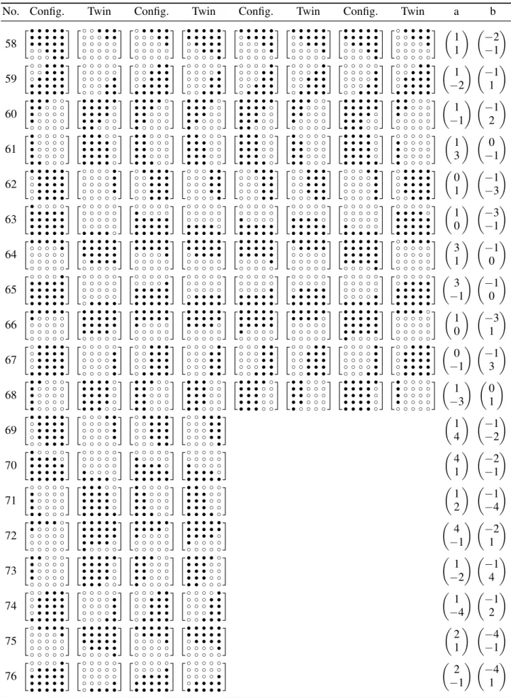
Table 5.The 92 groups of informative 5 5 con gurations (continued).
No. Config. Twin Config. Twin Config. Twin Config. Twin a b
20 • ◦ ◦ ◦ ◦ • ◦ ◦ ◦ ◦ ◦ ◦ ◦ ◦ ◦ ◦ ◦ ◦ ◦ ◦ ◦ ◦ ◦ ◦ ◦ • • • • • • • • • • • • • • • • • • • ◦ • • • • ◦ 1 −1 0 1 21 ◦ ◦ ◦ ◦ ◦ ◦ ◦ ◦ ◦ ◦ • ◦ ◦ ◦ ◦ • • ◦ ◦ ◦ • • • ◦ ◦ • • ◦ ◦ ◦ • • • ◦ ◦ • • • • ◦ • • • • • • • • • • 3 2 −2 −3 22 ◦ ◦ ◦ ◦ ◦ ◦ ◦ ◦ ◦ ◦ ◦ ◦ ◦ ◦ • ◦ ◦ ◦ • • ◦ ◦ • • • ◦ ◦ ◦ • • ◦ ◦ • • • ◦ • • • • • • • • • • • • • • 2
−3 −
3 2 23 ◦ ◦ • • • ◦ ◦ ◦ • • ◦ ◦ ◦ ◦ • ◦ ◦ ◦ ◦ ◦ ◦ ◦ ◦ ◦ ◦ • • • • • • • • • • ◦ • • • • ◦ ◦ • • • ◦ ◦ ◦ • • 2 3 −3 −2 24 • • • ◦ ◦ • • ◦ ◦ ◦ • ◦ ◦ ◦ ◦ ◦ ◦ ◦ ◦ ◦ ◦ ◦ ◦ ◦ ◦ • • • • • • • • • • • • • • ◦ • • • ◦ ◦ • • ◦ ◦ ◦ 3
−2 −
2 3 25 ◦ ◦ ◦ ◦ ◦ ◦ ◦ ◦ ◦ ◦ • ◦ ◦ ◦ ◦ • ◦ ◦ ◦ ◦ • • ◦ ◦ ◦ • • • ◦ ◦ • • • • ◦ • • • • ◦ • • • • • • • • • • 1 1 −1 −3 26 ◦ ◦ ◦ ◦ ◦ ◦ ◦ ◦ ◦ ◦ ◦ ◦ ◦ ◦ ◦ • ◦ ◦ ◦ ◦ • • • ◦ ◦ • • ◦ ◦ ◦ • • • • ◦ • • • • • • • • • • • • • • • 3 1 −1 −1 27 ◦ ◦ ◦ ◦ ◦ ◦ ◦ ◦ ◦ ◦ ◦ ◦ ◦ ◦ ◦ ◦ ◦ ◦ ◦ • ◦ ◦ • • • ◦ ◦ ◦ • • ◦ • • • • • • • • • • • • • • • • • • • 1
−1 −13 28 ◦ ◦ ◦ ◦ ◦ ◦ ◦ ◦ ◦ ◦ ◦ ◦ ◦ ◦ • ◦ ◦ ◦ ◦ • ◦ ◦ ◦ • • ◦ ◦ • • • ◦ • • • • ◦ • • • • • • • • • • • • • • 1
−3 −
1 1 29 ◦ ◦ ◦ • • ◦ ◦ ◦ ◦ • ◦ ◦ ◦ ◦ • ◦ ◦ ◦ ◦ ◦ ◦ ◦ ◦ ◦ ◦ • • • • • • • • • • ◦ • • • • ◦ • • • • ◦ ◦ • • • 1 3 −1 −1 30 ◦ ◦ • • • ◦ ◦ ◦ ◦ • ◦ ◦ ◦ ◦ ◦ ◦ ◦ ◦ ◦ ◦ ◦ ◦ ◦ ◦ ◦ • • • • • • • • • • • • • • • ◦ • • • • ◦ ◦ ◦ • • 1 1 −3 −1 31 • • • ◦ ◦ • ◦ ◦ ◦ ◦ ◦ ◦ ◦ ◦ ◦ ◦ ◦ ◦ ◦ ◦ ◦ ◦ ◦ ◦ ◦ • • • • • • • • • • • • • • • • • • • ◦ • • ◦ ◦ ◦ 3
−1 −
1 1 32 • • ◦ ◦ ◦ • ◦ ◦ ◦ ◦ • ◦ ◦ ◦ ◦ ◦ ◦ ◦ ◦ ◦ ◦ ◦ ◦ ◦ ◦ • • • • • • • • • • • • • • ◦ • • • • ◦ • • • ◦ ◦ 1
−1 −
1 3 33 ◦ ◦ ◦ ◦ ◦ • ◦ ◦ ◦ ◦ • • ◦ ◦ ◦ • • • ◦ ◦ • • • • ◦ • ◦ ◦ ◦ ◦ • • ◦ ◦ ◦ • • • ◦ ◦ • • • • ◦ • • • • • 4 3 −3 −4 34 ◦ ◦ ◦ ◦ ◦ ◦ ◦ ◦ ◦ • ◦ ◦ ◦ • • ◦ ◦ • • • ◦ • • • • ◦ ◦ ◦ ◦ • ◦ ◦ ◦ • • ◦ ◦ • • • ◦ • • • • • • • • • 3
−4 −
4 3 35 ◦ • • • • ◦ ◦ • • • ◦ ◦ ◦ • • ◦ ◦ ◦ ◦ • ◦ ◦ ◦ ◦ ◦ • • • • • ◦ • • • • ◦ ◦ • • • ◦ ◦ ◦ • • ◦ ◦ ◦ ◦ • 3 4 −4 −3 36 • • • • ◦ • • • ◦ ◦ • • ◦ ◦ ◦ • ◦ ◦ ◦ ◦ ◦ ◦ ◦ ◦ ◦ • • • • • • • • • ◦ • • • ◦ ◦ • • ◦ ◦ ◦ • ◦ ◦ ◦ ◦ 4
−3 −
Table 5. The 92 groups of informative 5 x 5 configurations (continued).
No. Config. Twin Config. Twin Config. Twin Config. Twin a b
39 ◦ ◦ ◦ ◦ ◦ ◦ ◦ ◦ ◦ ◦ ◦ ◦ ◦ ◦ ◦ ◦ ◦ ◦ • • • • • • • ◦ ◦ ◦ ◦ ◦ ◦ ◦ • • • • • • • • • • • • • • • • • • ◦ ◦ ◦ ◦ ◦ ◦ ◦ ◦ ◦ ◦ ◦ ◦ ◦ • • • • • • • • • • • • ◦ ◦ ◦ ◦ ◦ ◦ ◦ ◦ ◦ ◦ ◦ ◦ • • • • • • • • • • • • • ◦ ◦ ◦ ◦ ◦ ◦ ◦ ◦ • • • • • • • • • • • • • • • • • ◦ ◦ ◦ ◦ ◦ ◦ ◦ ◦ ◦ ◦ ◦ ◦ ◦ ◦ ◦ ◦ ◦ • • • • • • • • ◦ ◦ ◦ • • • • • • • • • • • • • • • • • • • • • • ◦ ◦ ◦ ◦ ◦ ◦ ◦ ◦ ◦ ◦ ◦ ◦ ◦ ◦ ◦ ◦ ◦ ◦ ◦ ◦ ◦ ◦ • • • 2
−1 −
1 0 40 ◦ ◦ ◦ ◦ • ◦ ◦ ◦ ◦ • ◦ ◦ ◦ ◦ • ◦ ◦ ◦ • • ◦ ◦ ◦ • • ◦ ◦ • • • ◦ ◦ • • • ◦ • • • • ◦ • • • • ◦ • • • • ◦ ◦ ◦ • • ◦ ◦ ◦ • • ◦ ◦ ◦ • • ◦ ◦ • • • ◦ ◦ • • • ◦ ◦ ◦ • • ◦ ◦ ◦ • • ◦ ◦ • • • ◦ ◦ • • • ◦ ◦ • • • ◦ ◦ • • • ◦ ◦ • • • ◦ ◦ • • • ◦ • • • • ◦ • • • • ◦ ◦ ◦ ◦ • ◦ ◦ ◦ ◦ • ◦ ◦ ◦ • • ◦ ◦ ◦ • • ◦ ◦ ◦ • • ◦ • • • • ◦ • • • • ◦ • • • • • • • • • • • • • • ◦ ◦ ◦ ◦ ◦ ◦ ◦ ◦ ◦ ◦ ◦ ◦ ◦ ◦ • ◦ ◦ ◦ ◦ • ◦ ◦ ◦ ◦ • 0
−1 −
1 2 41 ◦ ◦ ◦ • • ◦ ◦ ◦ • • ◦ ◦ ◦ ◦ • ◦ ◦ ◦ ◦ • ◦ ◦ ◦ ◦ • ◦ • • • • ◦ • • • • ◦ • • • • ◦ ◦ • • • ◦ ◦ • • • ◦ ◦ • • • ◦ ◦ • • • ◦ ◦ ◦ • • ◦ ◦ ◦ • • ◦ ◦ ◦ • • ◦ ◦ • • • ◦ ◦ • • • ◦ ◦ • • • ◦ ◦ ◦ • • ◦ ◦ ◦ • • ◦ • • • • ◦ • • • • ◦ ◦ • • • ◦ ◦ • • • ◦ ◦ • • • ◦ ◦ ◦ • • ◦ ◦ ◦ • • ◦ ◦ ◦ • • ◦ ◦ ◦ ◦ • ◦ ◦ ◦ ◦ • • • • • • • • • • • ◦ • • • • ◦ • • • • ◦ • • • • ◦ ◦ ◦ ◦ • ◦ ◦ ◦ ◦ • ◦ ◦ ◦ ◦ • ◦ ◦ ◦ ◦ ◦ ◦ ◦ ◦ ◦ ◦ 0 1 −1 −2 42 • • • • • ◦ ◦ ◦ • • ◦ ◦ ◦ ◦ ◦ ◦ ◦ ◦ ◦ ◦ ◦ ◦ ◦ ◦ ◦ • • • • • • • • • • • • • • • ◦ ◦ • • • ◦ ◦ ◦ ◦ ◦ • • • • • • • • • • ◦ ◦ ◦ • • ◦ ◦ ◦ ◦ ◦ ◦ ◦ ◦ ◦ ◦ • • • • • • • • • • ◦ ◦ • • • ◦ ◦ ◦ ◦ ◦ ◦ ◦ ◦ ◦ ◦ • • • • • • • • • • • • • • • ◦ ◦ ◦ • • ◦ ◦ ◦ ◦ ◦ • • • • • ◦ ◦ • • • ◦ ◦ ◦ ◦ ◦ ◦ ◦ ◦ ◦ ◦ ◦ ◦ ◦ ◦ ◦ • • • • • • • • • • • • • • • • • • • • ◦ ◦ ◦ • • ◦ ◦ • • • ◦ ◦ ◦ ◦ ◦ ◦ ◦ ◦ ◦ ◦ ◦ ◦ ◦ ◦ ◦ ◦ ◦ ◦ ◦ ◦ 2 1 −1 0 43 • • • • • • • ◦ ◦ ◦ ◦ ◦ ◦ ◦ ◦ ◦ ◦ ◦ ◦ ◦ ◦ ◦ ◦ ◦ ◦ • • • • • • • • • • • • • • • • • • ◦ ◦ ◦ ◦ ◦ ◦ ◦ • • • • • • • • • • • • ◦ ◦ ◦ ◦ ◦ ◦ ◦ ◦ ◦ ◦ ◦ ◦ ◦ • • • • • • • • • • • • • ◦ ◦ ◦ ◦ ◦ ◦ ◦ ◦ ◦ ◦ ◦ ◦ • • • • • • • • • • • • • • • • • ◦ ◦ ◦ ◦ ◦ ◦ ◦ ◦ • • • • • • • • ◦ ◦ ◦ ◦ ◦ ◦ ◦ ◦ ◦ ◦ ◦ ◦ ◦ ◦ ◦ ◦ ◦ • • • • • • • • • • • • • • • • • • • • • • ◦ ◦ ◦ • • • ◦ ◦ ◦ ◦ ◦ ◦ ◦ ◦ ◦ ◦ ◦ ◦ ◦ ◦ ◦ ◦ ◦ ◦ ◦ ◦ ◦ ◦ 1 0 −2 1 44 • • ◦ ◦ ◦ • • ◦ ◦ ◦ • ◦ ◦ ◦ ◦ • ◦ ◦ ◦ ◦ • ◦ ◦ ◦ ◦ • • • • ◦ • • • • ◦ • • • • ◦ • • • ◦ ◦ • • • ◦ ◦ • • • ◦ ◦ • • • ◦ ◦ • • ◦ ◦ ◦ • • ◦ ◦ ◦ • • ◦ ◦ ◦ • • • ◦ ◦ • • • ◦ ◦ • • • ◦ ◦ • • ◦ ◦ ◦ • • ◦ ◦ ◦ • • • • ◦ • • • • ◦ • • • ◦ ◦ • • • ◦ ◦ • • • ◦ ◦ • • ◦ ◦ ◦ • • ◦ ◦ ◦ • • ◦ ◦ ◦ • ◦ ◦ ◦ ◦ • ◦ ◦ ◦ ◦ • • • • • • • • • • • • • • ◦ • • • • ◦ • • • • ◦ • ◦ ◦ ◦ ◦ • ◦ ◦ ◦ ◦ • ◦ ◦ ◦ ◦ ◦ ◦ ◦ ◦ ◦ ◦ ◦ ◦ ◦ ◦ 1 −2 0 1 45 • ◦ ◦ ◦ ◦ • ◦ ◦ ◦ ◦ • • ◦ ◦ ◦ • • ◦ ◦ ◦ • • • ◦ ◦ • • ◦ ◦ ◦ • • • ◦ ◦ • • • ◦ ◦ • • • • ◦ • • • • ◦ ◦ ◦ ◦ ◦ ◦ • ◦ ◦ ◦ ◦ • ◦ ◦ ◦ ◦ • • ◦ ◦ ◦ • • ◦ ◦ ◦ • • • ◦ ◦ • • • ◦ ◦ • • • • ◦ • • • • ◦ • • • • • • • ◦ ◦ ◦ • • ◦ ◦ ◦ • • • ◦ ◦ • • • ◦ ◦ • • • • ◦ • ◦ ◦ ◦ ◦ • • ◦ ◦ ◦ • • ◦ ◦ ◦ • • • ◦ ◦ • • • ◦ ◦ 2 3 −1 −3 46 • • • • • ◦ • • • • ◦ • • • • ◦ ◦ • • • ◦ ◦ • • • ◦ ◦ ◦ • • ◦ ◦ ◦ • • ◦ ◦ ◦ ◦ • ◦ ◦ ◦ ◦ • ◦ ◦ ◦ ◦ ◦ ◦ • • • • ◦ ◦ • • • ◦ ◦ • • • ◦ ◦ ◦ • • ◦ ◦ ◦ • • ◦ ◦ • • • ◦ ◦ • • • ◦ ◦ ◦ • • ◦ ◦ ◦ • • ◦ ◦ ◦ ◦ • ◦ • • • • ◦ • • • • ◦ ◦ • • • ◦ ◦ • • • ◦ ◦ ◦ • • ◦ ◦ • • • ◦ ◦ ◦ • • ◦ ◦ ◦ • • ◦ ◦ ◦ ◦ • ◦ ◦ ◦ ◦ • 1 3 −2 −3 47 • ◦ ◦ ◦ ◦ • • • ◦ ◦ • • • • • • • • • • • • • • • ◦ ◦ ◦ ◦ ◦ ◦ ◦ ◦ ◦ ◦ ◦ ◦ ◦ ◦ ◦ • • ◦ ◦ ◦ • • • • ◦ ◦ ◦ ◦ ◦ ◦ • ◦ ◦ ◦ ◦ • • • ◦ ◦ • • • • • • • • • • ◦ ◦ ◦ ◦ ◦ ◦ ◦ ◦ ◦ ◦ • • ◦ ◦ ◦ • • • • ◦ • • • • • ◦ ◦ ◦ ◦ ◦ ◦ ◦ ◦ ◦ ◦ • ◦ ◦ ◦ ◦ • • • ◦ ◦ • • • • • ◦ ◦ ◦ ◦ ◦ • • ◦ ◦ ◦ • • • • ◦ • • • • • • • • • • 3 1 −3 −2 48 • • • • • ◦ ◦ • • • ◦ ◦ ◦ ◦ • ◦ ◦ ◦ ◦ ◦ ◦ ◦ ◦ ◦ ◦ • • • • • • • • • • ◦ • • • • ◦ ◦ ◦ • • ◦ ◦ ◦ ◦ ◦ • • • • • • • • • • ◦ ◦ • • • ◦ ◦ ◦ ◦ • ◦ ◦ ◦ ◦ ◦ • • • • • ◦ • • • • ◦ ◦ ◦ • • ◦ ◦ ◦ ◦ ◦ ◦ ◦ ◦ ◦ ◦ • • • • • • • • • • • • • • • ◦ ◦ • • • ◦ ◦ ◦ ◦ • ◦ • • • • ◦ ◦ ◦ • • ◦ ◦ ◦ ◦ ◦ ◦ ◦ ◦ ◦ ◦ ◦ ◦ ◦ ◦ ◦ 3 2 −3 −1 49 ◦ ◦ ◦ ◦ • ◦ ◦ • • • • • • • • • • • • • • • • • • ◦ ◦ ◦ ◦ ◦ ◦ ◦ ◦ ◦ ◦ ◦ ◦ ◦ ◦ ◦ ◦ ◦ ◦ • • ◦ • • • • ◦ ◦ ◦ ◦ ◦ ◦ ◦ ◦ ◦ • ◦ ◦ • • • • • • • • • • • • • ◦ ◦ ◦ ◦ ◦ ◦ ◦ ◦ ◦ ◦ ◦ ◦ ◦ • • ◦ • • • • • • • • • ◦ ◦ ◦ ◦ ◦ ◦ ◦ ◦ ◦ ◦ ◦ ◦ ◦ ◦ • ◦ ◦ • • • • • • • • ◦ ◦ ◦ ◦ ◦ ◦ ◦ ◦ • • ◦ • • • • • • • • • • • • • • 3
−2 −13 50 • • • • • • • • ◦ ◦ • ◦ ◦ ◦ ◦ ◦ ◦ ◦ ◦ ◦ ◦ ◦ ◦ ◦ ◦ • • • • • • • • • • • • • • ◦ • • ◦ ◦ ◦ ◦ ◦ ◦ ◦ ◦ • • • • • • • • • • • • • ◦ ◦ • ◦ ◦ ◦ ◦ ◦ ◦ ◦ ◦ ◦ • • • • • • • • • ◦ • • ◦ ◦ ◦ ◦ ◦ ◦ ◦ ◦ ◦ ◦ ◦ ◦ ◦ • • • • • • • • • • • • • • • • • • ◦ ◦ • ◦ ◦ ◦ ◦ • • • • ◦ • • ◦ ◦ ◦ ◦ ◦ ◦ ◦ ◦ ◦ ◦ ◦ ◦ ◦ ◦ ◦ ◦ ◦ ◦ 3
−1 −
3 2 51 • • ◦ ◦ ◦ • • ◦ ◦ ◦ • ◦ ◦ ◦ ◦ • ◦ ◦ ◦ ◦ ◦ ◦ ◦ ◦ ◦ • • • • • • • • • ◦ • • • • ◦ • • • ◦ ◦ • • • ◦ ◦ • • • ◦ ◦ • • ◦ ◦ ◦ • • ◦ ◦ ◦ • ◦ ◦ ◦ ◦ • ◦ ◦ ◦ ◦ • • • • ◦ • • • • ◦ • • • ◦ ◦ • • • ◦ ◦ • • ◦ ◦ ◦ • • • ◦ ◦ • • • ◦ ◦ • • ◦ ◦ ◦ • • ◦ ◦ ◦ • ◦ ◦ ◦ ◦ • • • • ◦ • • • ◦ ◦ • • • ◦ ◦ • • ◦ ◦ ◦ • • ◦ ◦ ◦ 2
−3 −
1 3 52 ◦ ◦ • • • ◦ ◦ • • • ◦ • • • • ◦ • • • • • • • • • ◦ ◦ ◦ ◦ ◦ ◦ ◦ ◦ ◦ • ◦ ◦ ◦ ◦ • ◦ ◦ ◦ • • ◦ ◦ ◦ • • ◦ ◦ ◦ • • ◦ ◦ • • • ◦ ◦ • • • ◦ • • • • ◦ • • • • ◦ ◦ ◦ ◦ • ◦ ◦ ◦ ◦ • ◦ ◦ ◦ • • ◦ ◦ ◦ • • ◦ ◦ • • • ◦ ◦ ◦ • • ◦ ◦ ◦ • • ◦ ◦ • • • ◦ ◦ • • • ◦ • • • • ◦ ◦ ◦ ◦ • ◦ ◦ ◦ • • ◦ ◦ ◦ • • ◦ ◦ • • • ◦ ◦ • • • 1
−3 −
2 3 53 • • • • • ◦ • • • • ◦ ◦ • • • ◦ ◦ • • • ◦ ◦ ◦ • • ◦ ◦ • • • ◦ ◦ ◦ • • ◦ ◦ ◦ • • ◦ ◦ ◦ ◦ • ◦ ◦ ◦ ◦ ◦ • • • • • • • • • • ◦ • • • • ◦ ◦ • • • ◦ ◦ • • • ◦ ◦ ◦ • • ◦ ◦ ◦ • • ◦ ◦ ◦ ◦ • ◦ ◦ ◦ ◦ ◦ ◦ ◦ ◦ ◦ ◦ ◦ • • • • ◦ ◦ • • • ◦ ◦ ◦ • • ◦ ◦ ◦ • • ◦ ◦ ◦ ◦ • ◦ • • • • ◦ ◦ • • • ◦ ◦ • • • ◦ ◦ ◦ • • ◦ ◦ ◦ ◦ • ◦ ◦ • • • ◦ ◦ ◦ • • ◦ ◦ ◦ ◦ • ◦ ◦ ◦ ◦ • ◦ ◦ ◦ ◦ ◦ • • • • • ◦ • • • • ◦ • • • • ◦ ◦ • • • ◦ ◦ ◦ • • 1 2 −1 −1 54 • ◦ ◦ ◦ ◦ • • ◦ ◦ ◦ • • • • ◦ • • • • • • • • • • ◦ ◦ ◦ ◦ ◦ ◦ ◦ ◦ ◦ ◦ • ◦ ◦ ◦ ◦ • • • ◦ ◦ • • • • ◦ ◦ ◦ ◦ ◦ ◦ • ◦ ◦ ◦ ◦ • • ◦ ◦ ◦ • • • • ◦ • • • • • ◦ ◦ ◦ ◦ ◦ • ◦ ◦ ◦ ◦ • • • ◦ ◦ • • • • ◦ • • • • • ◦ ◦ ◦ ◦ ◦ ◦ ◦ ◦ ◦ ◦ • ◦ ◦ ◦ ◦ • • ◦ ◦ ◦ • • • • ◦ • ◦ ◦ ◦ ◦ • • • ◦ ◦ • • • • ◦ • • • • • • • • • • • • ◦ ◦ ◦ • • • ◦ ◦ • • • • • • • • • • • • • • • ◦ ◦ ◦ ◦ ◦ ◦ ◦ ◦ ◦ ◦ ◦ ◦ ◦ ◦ ◦ • • ◦ ◦ ◦ • • • ◦ ◦ 2 1 −1 −1 55 ◦ ◦ ◦ ◦ ◦ • ◦ ◦ ◦ ◦ • ◦ ◦ ◦ ◦ • • ◦ ◦ ◦ • • • ◦ ◦ • • ◦ ◦ ◦ • • • ◦ ◦ • • • • ◦ • • • • ◦ • • • • • • ◦ ◦ ◦ ◦ • • ◦ ◦ ◦ • • ◦ ◦ ◦ • • • ◦ ◦ • • • • ◦ • ◦ ◦ ◦ ◦ • • ◦ ◦ ◦ • • • ◦ ◦ • • • ◦ ◦ • • • • ◦ • • • ◦ ◦ • • • ◦ ◦ • • • • ◦ • • • • • • • • • • ◦ ◦ ◦ ◦ ◦ ◦ ◦ ◦ ◦ ◦ • ◦ ◦ ◦ ◦ • • ◦ ◦ ◦ • • ◦ ◦ ◦ • • ◦ ◦ ◦ • • • ◦ ◦ • • • ◦ ◦ • • • • ◦ • • • • • ◦ ◦ ◦ ◦ ◦ • ◦ ◦ ◦ ◦ • • ◦ ◦ ◦ • • ◦ ◦ ◦ • • • ◦ ◦ 1 1 −1 −2 56 ◦ ◦ ◦ • • ◦ ◦ • • • • • • • • • • • • • • • • • • ◦ ◦ ◦ ◦ ◦ ◦ ◦ ◦ ◦ ◦ ◦ ◦ ◦ ◦ ◦ ◦ ◦ ◦ • • ◦ ◦ • • • ◦ ◦ ◦ ◦ • ◦ ◦ ◦ • • ◦ • • • • • • • • • • • • • • ◦ ◦ ◦ ◦ ◦ ◦ ◦ ◦ ◦ ◦ ◦ ◦ ◦ ◦ • ◦ ◦ • • • ◦ • • • • ◦ ◦ ◦ ◦ ◦ ◦ ◦ ◦ ◦ • ◦ ◦ ◦ • • ◦ • • • • • • • • • ◦ ◦ ◦ ◦ ◦ ◦ ◦ ◦ ◦ • ◦ ◦ • • • ◦ • • • • • • • • • ◦ ◦ ◦ ◦ ◦ ◦ ◦ ◦ ◦ ◦ ◦ ◦ ◦ ◦ • ◦ ◦ ◦ • • ◦ • • • • ◦ ◦ ◦ ◦ • ◦ ◦ • • • ◦ • • • • • • • • • • • • • • 1
−1 −
2 1 57 • • • • ◦ • • ◦ ◦ ◦ • ◦ ◦ ◦ ◦ ◦ ◦ ◦ ◦ ◦ ◦ ◦ ◦ ◦ ◦ • • • • • • • • • • • • • • ◦ • • • ◦ ◦ • ◦ ◦ ◦ ◦ • • • • • • • • • ◦ • • ◦ ◦ ◦ • ◦ ◦ ◦ ◦ ◦ ◦ ◦ ◦ ◦ • • • • • • • • • ◦ • • • ◦ ◦ • ◦ ◦ ◦ ◦ ◦ ◦ ◦ ◦ ◦ • • • • • • • • • • • • • • ◦ • • ◦ ◦ ◦ • ◦ ◦ ◦ ◦ • • • • ◦ • • • ◦ ◦ • ◦ ◦ ◦ ◦ ◦ ◦ ◦ ◦ ◦ ◦ ◦ ◦ ◦ ◦ • • • • • • • • • • • • • • • • • • ◦ ◦ • • ◦ ◦ ◦ • • • ◦ ◦ • • ◦ ◦ ◦ ◦ ◦ ◦ ◦ ◦ ◦ ◦ ◦ ◦ ◦ ◦ ◦ ◦ ◦ ◦ 2
−1 −
1 1