A COUNTING PROCESS WITH GENERALIZED
EXPONENTIAL INTER-ARRIVAL TIMES
Sahana Bhattacharjee1
Department of Statistics, Gauhati University, Guwahati, Assam, India
1. INTRODUCTION
The Poisson process is one of the most popular counting processes, which is based on the postulates viz. stationary and independent increments and the number of events in any interval of length ‘t’ is Poisson distributed with mean ‘λt’, whereλis the mean number of occurrences per unit time (Ross, 1995). Another important characteristic of the Poisson process is that the inter-arrival times are exponentially distributed. It has found extensive applications in queuing theory (Kingman, 1963), modeling scoring in a hockey game (DeJardine, 2013), modeling vehicles involved in road toll (Vong, 2013) etc.
However, the Poisson count model suffers from a major drawback of being valid only when the underlying data is equi-dispersed, i.e. when the mean and variance of the count data are the same (McShaneet al., 2008). This limitation has been addressed by many statisticians and over the years, count models have been developed which allow modeling of over-dispersed data (variance greater than the mean) and under-dispersed data (mean greater than the variance). A heterogeneous gamma Poisson or the negative binomial count model is the oldest model which addressed the issue of over-dispersion. Out of the several models developed for handling under-dispersed data, the one proposed by Winkelmann (1995) is based on gamma distributed inter-arrival times, which beau-tifully explores the Poisson-exponential connection. McShaneet al.(2008) proposed a count model assuming Weibull distributed inter-arrival times, which handles both over-dispersed and under-over-dispersed data. Also, this model nests the Poisson model and the negative binomial count model as special cases.
The inter-arrival time of the Poisson count model is exponentially distributed, and so, has a constant hazard function. But in real-life, the hazard may not remain con-stant over time. In such a case, the Poisson model will not be appropriate. The hazard function which expresses the instantaneous exit probability, conditional on survival,
captures the underlying time dependence of the count model (Jose and Abraham, 2013). Winkelmann (1995) carried out an extensive analysis of the timing model hazard func-tion and the dispersion in the equivalent count model and found that a decreasing haz-ard function (corresponding to negative duration dependence of the inter-arrival time distribution) leads to an over-dispersed count model, an increasing hazard function (cor-responding to positive duration dependence) leads to an under-dispersed count model and a constant hazard function (corresponding to no duration dependence) leads to an equi-dispersed count model (Jose and Abraham, 2011). Thus, a new count model can be derived by assuming some other inter-arrival time distribution, which possesses a non-constant hazard function.
In this paper, a new generalized count model is developed assuming the generalized exponential (GE) distribution as the inter-arrival time distribution, of which the expo-nential distribution is a special case. A corresponding count model is formulated which nests the traditional Poisson count model. The advantage of using the GE distribution over the exponential distribution is that the hazard function is non-constant and hence, the distribution is duration dependent. This allows the corresponding count model to account for over-dispersed and under-dispersed data. Some properties of the new pro-posed model are explored and simulation from the model is carried out. Finally, the application of the new model is illustrated with the help of two real-life data sets.
2. GENERALIZED EXPONENTIAL DISTRIBUTION
The three-parameter generalized exponential (GE) distribution (the parameters being location, scale and shape parameter) was proposed by Gupta and Kundu (1999), as an alternative to the gamma and Weibull distribution. The gamma distribution has the lim-itation of not having a closed form of the cumulative distribution function (and hence, the survival functions and the hazard function). The Weibull distribution, although has a easily computable form of the cumulative distribution, survival and hazard function, does not possess the likelihood ratio ordering property. In addition, there does not ex-ist a UMP test for testing the one-sided hypothesis on the shape parameter when the other two parameters are known. The GE distribution takes care of these limitations and have properties similar to those of gamma and Weibull distribution. It has found use in analyzing lifetime data and in the field of medical science, among numerous other applications.
The random variableX has a GE distribution with parametersα,λandµif it has the distribution function
FGE(x;α,λ,µ) =h1−expn−x−λµoiα x> µ,α,λ >0. (1)
The density function corresponding to the distribution function (1) is fGE(x;α,λ,µ) =α
λ
h
1−expn−x−µ
λ
oiα−1
expn−x−µ
λ
o
Here,α,λ,µis the shape parameter, scale parameter and location parameter respec-tively and it is denoted by GE(α,λ,µ).
Puttingα=1 andµ=0 in (2) yields the p.d.f of the exponential distribution with scale parameterλ, which is
f(x;λ) = 1
λexp
−x
λ
. (3)
As discussed in Gupta and Kundu (1999), the hazard function of the GE(α,λ, 0) dis-tribution is given by
h(x;α,λ, 0) =α
λ
1−e−xλα−1 e−λx
1−1−e−xλα .
h(x;α,λ, 0)is an increasing function ifα <1, a decreasing function forα >1 and con-stant for α= 1. The same authors have displayed the use of the GE distribution in modeling the endurance of deep groove ball bearings.
3. GENERALIZED EXPONENTIAL COUNT MODEL
LetZndenotes the interval between the(n−1)t handnt hoccurrence of a process{N(t), t≥0}and let the sequenceZ1,Z2, . . . ,Znbe independently and identically distributed random variables having the GE(α,1,0) distribution. Then, the sumWn=Z1+Z2+. . .+ Znrepresents the waiting time up to thent h occurrence or the time from the origin of the process to thent hsubsequent occurrence.
IfZ0
isare independently and identically distributed such thatZi∼GE(α, 1, 0), then it can be seen thatZ =Pni=1Zi has the density function given by (Gupta and Kundu, 1999)
gZ(z) = X∞ j=0
Cj(nα+j)exp(−z){1−exp(−z)}nα+j−1
= X∞
j=0
CjfGE(z;nα+j, 1, 0) (4)
where the constantsCjare defined as C0=[ΓΓ((1α+n+1α)])n,Cj= C0nα
(nα+j)C(n)j ;j=1, 2, . . . ,C (2) j = [
(α)j]
2
j!(2α)j,
Cj(k)=({k−1}α)j
(kα)j
Pj i=0
(α)i
i! C (k−1)
Thus,Wn, the waiting time up to thent h occurrence of the process{N(t),t≥0} has the density function given in (4). The distribution function of the waiting timeWn is given by
Fw
n(t) = P{Wn≤t}
= 1−P(Wn(t)}
= 1−P{N(t)<n} = 1−P{N(t)≤(n−1)}
= 1−FN(t)(n−1). Therefore
FN(t)(n−1) = 1−Fw
n(t)
= 1−
∞
X
j=0
Cj{1−exp(−t)}nα+j. (5)
Finally, the probability law ofN(t)is pn(t) = P{N(t) =n}
= FN(t)(n)−FN(t)(n−1)
= 1−
∞
X
j=0
Cj{1−exp(−t)}(n+1)α+j−1+
∞
X
j=0
Cj{1−exp(−t)}nα+j
= X∞
j=0
Cj{1−exp(−t)}nα+j[1− {1−exp(−t)}α].
THEOREM1. If the inter-arrival times are independently and identically distributed as generalized exponential distribution with parametersα,λ=1andµ=0, then the count model probabilities are given by
pn(t) =P{N(t) =n}= ∞
X
j=0
Cj{1−exp(−t)}nα+j[1− {1−exp(−t)}α], (6)
where C0=[ΓΓ((α1+n+1α)])n,Cj= C0nα
(nα+j)Cj(n);j=1, 2, . . . ,C (2) j = [
(α)j]
2
j!(2α)j,
Cj(k)=({k−1}α)j
(kα)j
Pj i=0
(α)i
i! C (k−1)
j−i ;k=3, . . .n.
In particular, whenα=1, the count model probabilities in (6) reduce to pn(t) =P{N(t) =n}=
∞
X
j=0
where
C0= 1
Γ(1+n), Cj= C0n
(n+j)C (n)
j ; j=1, 2, . . . , Cj(2)= [Γ(1+j)]
2
j!(2)j , C (k) j =
(k−1)j
(k)j j X
i=0
Γ(1+i) i! C
(k−1)
j−i , k=3, . . .n, which is the probability function of Poisson distribution with unit rate parameter.
3.1. Characteristics of the generalized exponential count model
1. The model handles both over-dispersed and under-dispersed data
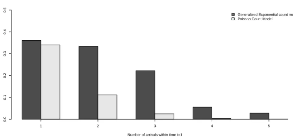
The hazard function of the GE distribution is a decreasing function of time whenα <1 and so, the distribution displays negative duration dependence. This, in turn, causes over-dispersion in the generalized exponential count model. Forα >1, the hazard func-tion is an increasing funcfunc-tion of time, so that the distribufunc-tion displays positive durafunc-tion dependence and causes under-dispersion in the generalized exponential count model. There is no duration dependence whenα= 1, which gives the Poisson count model having equal mean and variance. Figure 1 shows the hazard rate plot of GE(α,λ,0) for different values ofαandλ=1, which supports this result. As a validation of these
find-Figure 1 –Hazard rate plot of GE(α,λ,0) for different values ofαandλ=1.
ings, Figures 2 and 3 display the probability functions for the generalized exponential and Poisson count models for different parameter values. In both the cases, the general-ized exponential and Poisson models are chosen so as to have identical means.
of the model in this case is smaller than the mean. Figure 3 displays the over-dispersed generalized exponential model withα=0.5 and Poisson model with mean 0.655 and the variance of the model in this case is greater than the mean, as expected.
1 2 3 4 5
Number of arrivals within time t=1
Probability
0.0
0.2
0.4
0.6
0.8
Generalized Exponential count model Poisson Count Model
Figure 2 –Probability function for the generalized exponential model(α=1.5)and Poisson count model (mean=0.566), displaying under dispersion.
1 2 3 4 5
Number of arrivals within time t=1
Probability
0.0
0.1
0.2
0.3
0.4
0.5
Generalized Exponential count model Poisson Count Model
2. The model is computationally feasible to work with and the probabilities and moments can be estimated without taking resort to time-consuming simulation based methods
The summations which appear in the expressions for the count model probabilities, its mean and variance, are not quite sensitive to the number of terms which are used in sum-mations to approximate the values. The required number of terms is easily identifiable through empirical testing. Therefore, the count model probabilities and mean, variance of the count model can be conveniently estimated.
3. Researchers who deal with data having GE inter arrival times now have a cor-responding count model to use
Equation (6) shows the count model probabilities when the inter arrival time isGE(α, 1, 0,t), and thus, the link between the timing model and its count model is maintained. Using this link between the timing model and the count model, one can also predict the next inter arrival time, when only the count data is available.
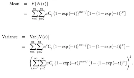
4. The mean and variance of the generalized exponential count model exist The mean and variance of the model exist and are given by
Mean = E[N(t)]
= X∞
n=1
∞
X
j=0
nCj{1−exp(−t)}nα+j[1− {1−exp(−t)}α]
Variance = Var[N(t)]
= X∞
n=1
∞
X
j=0
n2Cj{1−exp(−t)}nα+j[1− {1−exp(−t)}α]−
∞
X
n=1
∞
X
j=0
nCj{1−exp(−t)}nα+j[1− {1−exp(−t)}α] !2
.
Table 1 gives the generalized exponential count model probabilities for different val-ues ofαatt=1, 2. The values are approximated by retaining 10 terms in the summation of the expression for count model probabilities in (6).
TABLE 1
Values of the generalized exponential count model probabilities for different values ofαat t=1, 2.
t=1 t=2
α P1(t) P2(t) P3(t) P1(t) P2(t) P3(t)
0.3 0.1380 0.0928 0.0717 0.0569 0.0385 0.0336 0.6 0.2543 0.1172 0.0615 0.1284 0.0653 0.0444 0.8 0.3138 0.1126 0.0440 0.1786 0.0764 0.0423 1 0.3382 0.1070 0.0358 0.2287 0.0827 0.0366 1.3 0.4033 0.0768 0.0133 0.3016 0.0849 0.0259 1.7 0.4271 0.0485 0.0042 0.3914 0.0784 0.0139 2 0.4259 0.0326 0.0016 0.4519 0.0696 0.0080
TABLE 2
Values of mean and variance of the generalized exponential count model for different values ofαat t=1, 2.
t=1 t=2
4. APPLICATION TO REAL DATA SETS
In this section, the application of the generalized exponential count model to two real data sets is shown. The simulation of the generalized exponential count model prob-abilities and calculation of its mean and variance are carried out using theRsoftware, version 3.4.0, through the user-contributed packages viz. reliaR(Kumar and Ligges, 2015) with the help of self-programmed codes. ThemaxLikpackage (Toomet and Hen-ningsen, 2015) is used to obtain the maximum likelihood estimates of the parameters of the inter-arrival time distribution.
4.1. Data set-I: Arrival of patients at a clinic
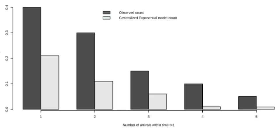
Data set-I is comprised of inter arrival times of patients arriving at a clinic situated at Adabari Tiniali, Guwahati, Assam, India on a given day. The time period of the collec-tion of data is from 07:00 PM to 09:00 PM, during which the concerned doctor attends to the patients. The inter-arrival times are positively skewed, having a long tail towards the right side of the peak and they are expressed in minutes. The number of patients ar-riving in the clinic on the randomly selected day is 32. It is further found that the there is usually very little gap between the arrival of consecutive customers, but in a very few instances, there is a considerable gap between the successive arrivals. In the data set considered, inter-arrival time exceeding 10 minutes or more is highly improbable.
The mean of the data set is found to be 0.53845 whereas the variance is found to be 0.57048. Given these information extracted from the data set, the goodness of fit test of theGE(α, 1, 0)distribution to the given data set is carried out. Assuming that the data set is from GE(α, 1, 0), the m.l.e ofαis found to be ˆα=0.50987. Now, to test the hypothesisH01 :GE(α, 1, 0)with ˆα=0.50987 is a good fit to the given data, the Kolmogorov-Smirnov one sample test is used. The p-value of the test is found to be 0.7075> 0.05. Hence, H01 is accepted at 5% level of significance and it is concluded that the assumption ofGE(α, 1, 0)distributed inter arrival times with ˆα=0.50987 is valid. Therefore, the number of patients arriving in an interval can be estimated using the over-dispersed generalized exponential count model.
Figure 4 shows the probability of observed counts and predicted generalized expo-nential model counts of patients arriving in the clinic in a time interval of length 1 minute.
4.2. Data set-II: Arrival of customers in a departmental store
1 2 3 4 5
Number of arrivals within time t=1
Probability
0.0
0.1
0.2
0.3
0.4
Observed count
Generalized Exponential model count
Figure 4 –Probability of observed counts and predicted generalized exponential model counts of patients arriving in the clinic.
1 2 3 4 5
Number of arrivals within time t=1
Probability
0.0
0.2
0.4
0.6
0.8
Observed count
Generalized Exponential model count
Figure 5 –Probability of observed counts and predicted generalized exponential model counts of customers arriving in the departmental store.
is not much gap between the arrival of the consecutive customers and only in a few instances, there is a fairly good gap between the successive arrivals. In the data set, inter-arrival time exceeding 8 minutes of more is highly unlikely.
ˆ
α=1.52752 is a good fit to the given data, the Kolmogorov-Smirnov one sample test is used. Thep-value of the test is found to be 0.3536>0.05. Hence,H02is accepted at 5% level of significance and it is concluded that the assumption ofGE(α, 1, 0)distributed inter arrival times with ˆα=1.52752 is valid. Therefore, the number of customers ar-riving in an interval can be estimated using the under-dispersed generalized exponential count model.
Figure 5 shows the probability of observed counts and predicted generalized expo-nential model counts of customers arriving in the departmental store in a time interval of length 1 minute.
5. CONCLUSION
In this article, a new count model based on generalized exponential (GE) inter arrival time process is introduced. This model is based on generalized exponentially distributed inter arrival times and is a generalization of the traditional Poisson count model. An-other advantage of this new model lies in its ability to model under-dispersed, equi-dispersed as well as over-equi-dispersed count data, owing to the non-constant hazard func-tion of the corresponding GE inter arrival time distribufunc-tion. The simulafunc-tion of count model probabilities and calculation of the mean and variance of the model can be car-ried out using theRsoftware. Finally, the proposed model is applied to two real life data sets, where the inter arrival times are generalized exponentially distributed. It is seen that the generalized exponential count model is able to model both over dispersed and under dispersed count data, in addition to the equi-dispersed count data.
6. ACKNOWLEDGEMENTS
I would like to thank the reviewers for their valuable comments which helped in signif-icantly improving the contents of the paper.
REFERENCES
Z. V. C. DEJARDINE (2013). Poisson Processes and Applications in Hockey. Lakehead University, Thunder Bay, Ontario, Canada. URL https://www.lakeheadu.ca/sites/default/files/uploads/77/docs/ DejardineFinal.pdf.
R. D. GUPTA, D. KUNDU(1999). Generalized exponential distributions. Australian & New Zealand Journal of Statistics, 41, no. 2, pp. 173–188.
K. K. JOSE, B. ABRAHAM (2011). A count model based on Mittag-Leffler interarrival times. Statistica, 71, no. 4, pp. 501–514.
J. F. C. KINGMAN(1963).Poisson counts for random sequences of events. The Annals of Mathematical Statistics, 34, no. 4, pp. 1217–1232.
V. KUMAR, U. LIGGES(2015). Package for some probability distributions. R package version 0.01, URL: https://cran.r-project.org/web/packages/reliaR/reliaR.pdf. B. MCSHANE, M. ADRIAN, E. T. BRADLOW, P. S. FADER(2008). Count models based
on Weibull interarrival times. Journal of Business and Economic Statistics, 26, no. 3, pp. 369–378.
S. M. ROSS(1995). Stochastic Processes. John Wiley & Sons, New York.
O. TOOMET, A. HENNINGSEN (2015). Maximum Likelihood Estima-tion and Related Tools. R package version 1.3-4, URL: https:// cran.r-project.org/web/packages/maxLik/maxLik.pdf.
I. K. VONG (2013). Theory of Poisson Point Process and its Application to Traffic Modelling. Department of Mathematics and Statistics, The University of Melbourne, Parkville, Victoria 3010, Australia. URL https://pdfs.semanticscholar.org/0044/7f6f9f3c2809934604c9f99c583 313e3f270.pdf.
R. WINKELMANN(1995). Duration dependence and dispersion in count data models. Journal of Business and Economic Statistics, 13, pp. 467–474.
SUMMARY
This paper introduces a new counting process which is based on generalized exponentially dis-tributed inter-arrival times. The advantage of this new count model over the existing Poisson count model is that the hazard function of the inter arrival time distribution is non-constant, so that the distribution is duration dependent and hence, is able to model both under dispersed and over dispersed count data, as opposed to the exponentially distributed inter arrival time of the Poisson count model, which is not duration dependent and the corresponding count model is able to model only equi-dispersed data. Further, some properties of this model are explored. Simulation from this new model is performed to study the behavior of count probabilities, mean and variance of the model for different values of the parameter. Use of the proposed model is illustrated with the help of real life data sets on arrival times of patients at a clinic and on arrival times of customers at a departmental store.