Dynamic decision-making under uncertainties: algorithms based on linear decision rules and applications in operating models

(1)

c

(2)

DYNAMIC DECISION-MAKING UNDER UNCERTAINTIES: ALGORITHMS BASED ON LINEAR DECISION RULES AND APPLICATIONS IN

OPERATING MODELS

BY LIMENG PAN

DISSERTATION

Submitted in partial fulfillment of the requirements

for the degree of Doctor of Philosophy in Systems and Entrepreneurial Engineering in the Graduate College of the

University of Illinois at Urbana-Champaign, 2014

Urbana, Illinois

Doctoral Committee:

Associate Professor Xin Chen, Chair Professor Ximing Cai

Associate Professor Carolyn L. Beck Associate Professor Qiong Wang

(3)

Abstract

This thesis is to propose efficient and robust algorithms based on Linear Decision Rule (LDR), which expand the applicability of the existing LDR methods. Representative and complex operation models are analyzed and solved by the proposed approaches. The research motivation and scope are provided in Chapter 1.

Chapter 2 introduces the generic LDR method and the contributions of this thesis to the LDR literature. To extend the LDR method to nonlinear objectives, two methods are proposed. The first is an iterative LDR (ILDR) method that tackles general concave differentiable nonlinear terms in the ob-jective function. The second treats quadratic terms in the obob-jective function by a Second-Order Cone approximation. The details and implementation of the proposed methods are presented in Chapter 3 and Chapter 4.

Chapter 3 utilizes the Robust Optimization approach to derive an ILDR solution for a multi-period hydropower generation problem that has a non-linear objective function. The methodology results in tractable second-order cone formulations. The performance of the ILDR approach is compared with the Sampling Stochastic Dynamic Programming (SSDP) policy derived using historical data.

In Chapter 4, a joint pricing and inventory control problem of a perishable product with a fixed lifetime is analyzed. Both the backlogging and lost-sales cases are discussed. The analytic results shed new light on perishable inventory management, and the proposed approach provides a significantly simpler proof of a classical structural result in the literature. Two heuristics were proposed, one of which is a modification and improvement of an exist-ing heuristic. The other one is an LDR based approach, which approximates the dynamics and the objective function by robust counterparts. The robust counterpart for the backlogging case is tight, and it leads to a satisfactory performance of less than 1% loss of optimality. Although the robust

(4)

coun-terpart for the lost-sales case is not tight in the current numerical study, the gap between the LDR method and the SDP benchmark is less than 5% on average.

Chapter 5 summarizes the contributions of the thesis and discusses about potential improvements. One important working project, an approximate dynamic programming based on LDR (ADP-LDR) approach, is introduced for future research.

(5)

(6)

Acknowledgments

I would like to sincerely thank my thesis committee members, Professor Car-olyn Beck, Professor Ximing Cai, Profess Xin Chen, and Professor Qiong Wang. Their valuable insights are critical to the success of this thesis.

I am indebted to my advisor Professor Xin Chen for guiding me on my research, study, and life in the past five years. Although words are not enough to express my gratitude, his wisdom, vision, generosity, and all the efforts should be acknowledged. Whenever I encounter obstacles, he always provides vital support. Before I established my specific research interest, he found proper papers for me to read. When I could not secure the Teaching Assistant financial support, he provided me with Research Assistantship even when I was not mature enough to handle the research problems. He organized research teams so I can learn while doing research. Without his expertise and kindness, it would take me much longer before I could conduct research independently. His efforts are especially appreciated given that he has a very busy schedule. In the mean time, as a wise, positive, and happy person, Professor Chen shares a lot of wonderful time with us at his home during holidays. In a word, it is really rewarding and enjoyable to be his student.

I want to especially thank Professor Ximing Cai, Professor Zhan Pang (Lancaster University, UK), Professor Pan Liu (Wuhan University, China), Dr. Mashor Housh, and Wenbo Chen, who are coauthors of my research papers. Besides the inspiring discussion, their expertise and inputs are im-portant part of this thesis. Professor Pang is a major contributor of the paper on perishables. He also gave me valuable advice on my career planning. Pro-fessor Cai guided me in two major revisions of the reservoir operations’ paper. Dr. Housh and Wenbo Chen are active researchers and good communicators. I learned a lot from all the coauthors.

While studying and working at the Department of Industrial and Enter-prise Systems Engineering, I was blessed with a wonderful line of

(7)

administra-tion: Professor Rakesh Nagi, Holly Kizer, Professor Ramavarapu Sreenivas, and many others. I sincerely thank these people for their dedicated work and valuable advice.

I am also very fortunate to meet friends such as Shahzad Bhatti, Jingnan Chen, Wenbo Chen, Zisheng Chen, Xiangyu Gao, Tinghao Guo, Peng Hu, Zhenyu Hu, Hao Jiang, Seyed Mohammad Nourbakhsh, Ross Peterson, Tyler Refsland, Dane Schiro, Xinxin Shu, Alok Tiwari, Katrina Underwood, Youyi Wei, Yunwen Xu, Fan Ye, Yuhan Zhang, Tao Zhu and many others.

Finally, I want to thank my family for their numerous sacrifices. My wife, Yuechang Mei, always gives me love and encouragement. This thesis could not have been finished without her support and sacrifices.

(8)

List of Tables

3.1 Policies comparison with consecutive historical inflows. . . 35

3.2 Policy Comparison with Consecutive Generated Inflows . . . . 38

3.3 Policies comparison with Trinity-Shasta inflows from Oc-tober 1912 to OcOc-tober 2012, recorded and artificially generated. 41 4.1 Demand models (a >0, b >0) . . . 66

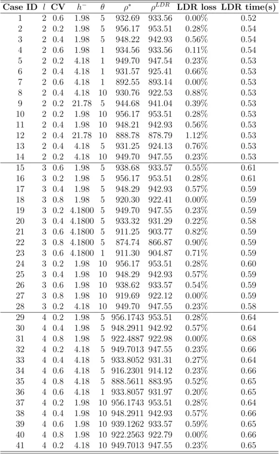
4.2 Case studies by LDR for backlogging models . . . 88

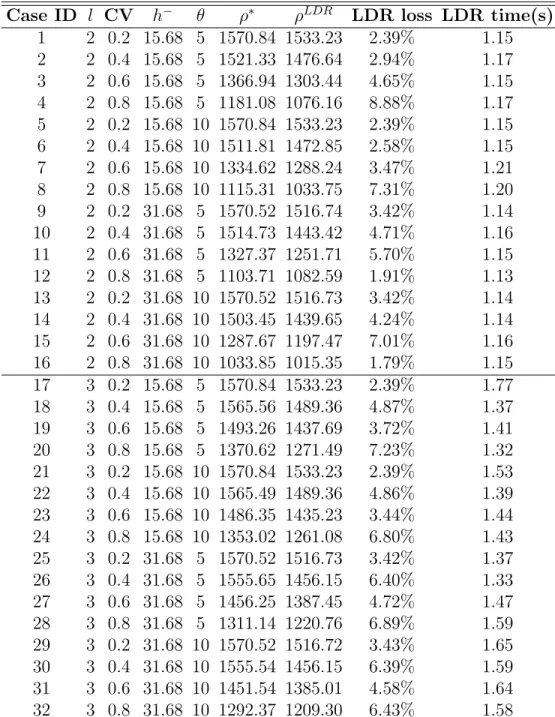
4.3 Case studies by LDR for lost-sales models . . . 89

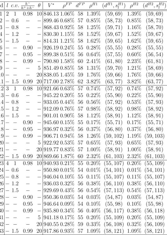
B.1 Long-Run Average Profits Per Period . . . 100

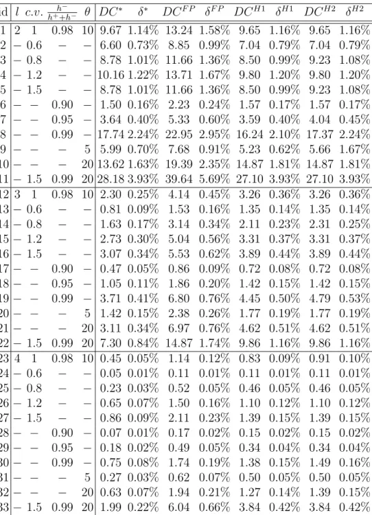
B.2 Average Disposal Costs Per Period . . . 101

B.3 Finite-Horizon Models with Non-Stationary Demand . . . 102

B.4 Average Costs and Disposal Costs Per Period for Cost-Minimization Problems . . . 103

(11)

List of Figures

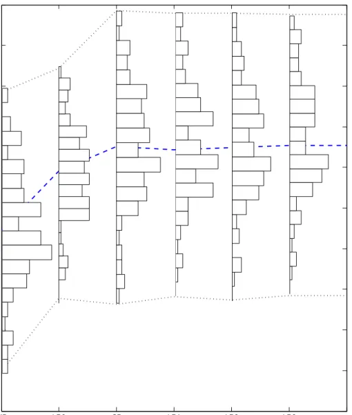
3.1 An example of segregation with Nt = 7 andτ4t≤qt≤τ5t. . . . 31 3.2 The location of the Three Gorges Reservoir basin in China. . . 33 3.3 Histogram comparison of the policies with consecutive

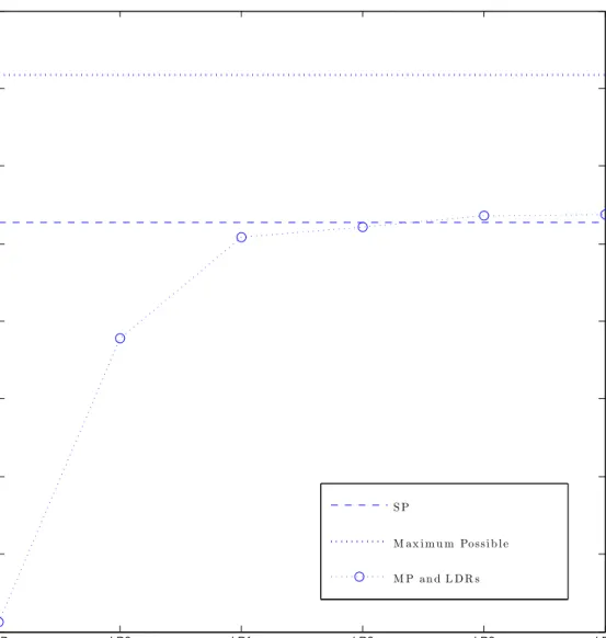
his-torical inflows. . . 36 3.4 The performance comparison of the policies on TGR with

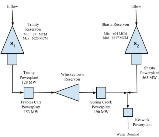
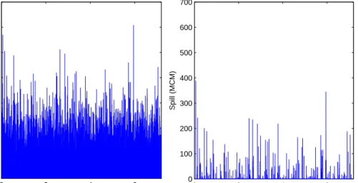
historical inflows.. . . 37 3.5 The schematic diagram of the Shasta-Trinity subsystem. . . . 42 3.6 Potential spills (infeasibility) from SSDP and LR4. . . 43

(12)

Chapter 1 Introduction

The research in this thesis is motivated by the complexity of dynamic deci-sion making under uncertainty and the limitations of the existing stochastic optimization solutions. Thus the intention of this thesis is twofold: to design generic methodologies for dynamic decision making under uncertainty and to model, analyze, and solve representative operation models.

1.1 Characterizing the Difficulties of Dynamic Decision

Making under Uncertainty

Dynamic decision making problems arise in many settings, from the control of an aircraft to the management of a retailer’s supply chain. In some en-gineering settings, the status of the system is continuously monitored and the decisions/actions can be made at any time in a continuous space. These problems are usually addressed by “control theory”. Alternatively, many other operation models, especially those for business management, consider discrete time decision making and only review the status of the system at discrete times. This thesis addresses problems in the latter setting. Given its generality, Dynamic decision making under uncertainty often faces four difficulties.

First, it is important to study dynamic decision making. Single period optimization does not solve all problems especially those concerning future. For example, a product may be very popular when it is introduced because it is a new technology electronic device or a fresh food product. Its value decreases as it becomes older. On the contrary, for instance, a product may become more popular as consumers become more familiar with it and get used to it. To plan the production, distribution and pricing of this product, its entire lifetime should be considered. The planning horizon can be long and

(13)

multiple decisions need to be made at different stages. Thus a multi-stage model is needed.

Second, it is important to incorporate randomness in the model, because randomness widely exists and so do the techniques to measure, collect, and access observations of randomness (i.e. data). Given the length of the plan-ning horizon, randomness usually comes up in operation models. Explicitly modeling uncertainties leads to more realistic models. Some randomness is from the physical world. For example, river flows of the coming week are stochastic. Others can come from human behaviors. Humans as consumers have been greatly liberalized by consistent gains in productivity and the market has become highly diversified because of the innovation of manu-facturers. Thus consumers have increasing freedom when consuming. This freedom combined with the nature of human behavior, leads to drastic uncer-tainties in the market. It may be argued that all parties in the supply chain, including the manufacturers, have more freedom due to the development of economy and technology. However, rational participants should transfer this freedom into profit by making correct decisions under uncertainty.

Uncertainties can be classified into two categories based on whether they will be revealed within the planning horizon. The degree of noise in the mea-surements of a physical instrument remains unknown until a more accurate physical instrument is applied. This type of uncertainty is not considered to be revealed by the planning horizon in this thesis. However, many other un-certainties will be revealed. For example, the reservoir inflows, the demand and supply capacities are revealed in the next stage. Recent advances in information technologies such as Enterprise Resource Planning (ERP) sys-tems and Radio-Frequency Identification (RFID) tags have enabled compa-nies to gather information about the observation of these revealed uncertain-ties from its supply chain more effectively and make real-time adjustment with a smaller amount of cost.

Third, the complex dynamic decision making under uncertainty problems usually lead to high dimensional state space in the model and put the “curse of dimensionality” obstacle on the path of solving these problems. Due to two factors, the dimension of the state variable in such problems is large. One reason is that the complexity of this problem requires a high dimen-sional variable to properly describe the state. For instance, a supermarket sells various categories of product; there are various brands and expiration

(14)

dates for each product category. At any time, a state variable in a space of thousands of dimensionality is needed to describe the inventory of this super-market. Actually, the supermarket also has a pipeline inventory that is being transported from their suppliers. The second reason is that the uncertainties are usually correlated. Time series analysis in our study by auto-regressive-moving-average (ARMA) and seasonal ARMA models show the data need to be modeled with a lag greater than 1. To properly incorporate this correla-tion in Stochastic Dynamic Programming (SDP), the dimension of the state variable can be significantly increased.

Lastly, the objective function in operation models can be nonlinear. For instance, to optimize the profit, we need to include the revenue term which is the product of sales and price. Sales and price are both affected by the operation policy, especially in a dynamic setting where the variables in the current stage are usually functions of the decisions in the past. Non-linearity in the complex stochastic dynamic setting is not trivial to tackle.

1.2 Research Scope

In the previous section, the difficulties of dynamic decision making under uncertainty have been characterized as: dynamic, stochastic, high dimen-sion, and non-linearity. This research focuses on developing algorithms and modeling methodologies to tackle these difficulties.

The uncertainties can be modeled in two approaches. The first assumes a probability distribution and optimizes the expected value of the objective function. This is a large and active research field. One good introduction can be found from (Birge and Louveaux 2011). The second approach is dis-tributionally robust and its result does not depend on the assumption of a specific distribution function. Instead, it only assumes the uncertainty’s dis-tribution belongs to a family of disdis-tributions that share certain properties: such as the support, the mean, and the covariance matrix. The problem is reformulated to optimize the outcome when the true distribution is the “worst” distribution member in this family. Notice that the outcome can be the expected value or the worst-case value. The former is a typical form of objective function in Stochastic Optimization; and the latter is a typical Robust Optimization objective function. Interested readers can refer to the

(15)

book (Ben-Tal et al. 2009) for comprehensive theory in Robust Optimization. There isn’t an absolute boundary between Stochastic and Robust Optimiza-tion. The methodology developed in this thesis belongs to their intersection: using the philosophy and skills of Robust Optimization to solve Stochastic Optimization problems.

The dynamics are modeled by discrete time multi-stage models. We focus on the second category of uncertainties, which are due to be revealed within the planning horizon and the decision to be made after the observation of the revealed uncertainties are called recourse decisions. The recourse decision should not be modeled as static variables because they are contingent on uncertainties revealed by the time this new decision is being made. To be more precise, the recourse decision is a function of the existing information. Although more realistic, modeling dynamic decision making in this way will exponentiate the complexity of resulting optimization problem. To solve it, a tractable approximation is needed. Linear Decision Rule (LDR) is a natural choice to approximate the recourse decision. There has been active research on this topic. This thesis answers some interesting research questions and proposes more versatile approaches which extend the capability of algorithms based LDR.

The approaches proposed in this thesis are applied to representative and difficult operation models and this forms the second line of our research. The models we selected are not only suitable for our methodology, but are also among those that raise interesting questions and draw attention from the research community. One application is about reservoir operations. The un-certain inflows are correlated and the objective function is nonlinear. Then another proposed method is applied to perishable inventory control and pric-ing. This is the first LDR approach that solves coordinated inventory control and pricing problems. Analysis and simplified proof are also obtained to char-acterize the properties of this complex dynamic system. Finally, to improve the accuracy, we propose the LDR based approximate dynamic programming approach (ADP-LDR). It is one of the most important research projects that I will continue to work on in the future.

(16)

1.3 Organization of the Thesis

Chapter 2 introduces the generic LDR method and our new approaches and findings. Existing LDR method is restricted to linear models: linear objective and linear constraints, except for the positive and negative parts: (·)+ ₌ max(0,·) and (·)− ₌ ₋_min(0_,_{·). Iterative Linear Decision Rule (ILDR)}

is proposed to solve a more general stochastic optimization problem with nonlinear objective function. When the nonlinear term is quadratic, such as the revenue term in coordinated pricing and inventory control problem. A neat second-order cone approximation is proposed.

Chapter 3 utilizes ILDR to solve the multi-stage reservoir operation prob-lem. The methodology results in tractable linear or nonlinear (Second-Order Cone) formulations. Both single and multi-reservoir systems are studied and the latter is an interesting and difficult problem recognized by the water re-source research community. The performance of the ILDR approach is com-pared with the Sampling Stochastic Dynamic Programming (SSDP) policy derived using historical data. The results show that the ILDR outperforms the SSDP policy when tested on generated data. At the same time the ILDR performs as well as the SSDP policy when tested on historical data. These results indicate that the proposed approach is both tractable and robust to the probability distribution of the uncertain data.

In Chapter 4, a joint pricing and inventory control problem of a perishable product with a fixed lifetime is analyzed. This is the first study of coordinated pricing and inventory control by LDR. The details of the SOC treatment of the quadratic term in the objective function is presented. Both the lost-sale and backlogging cases are discussed. Our analytic results shed new light on perishable inventory management, and our approach provides a significantly simpler proof of a classical structural result in the literature. Moreover, we identify bounds on the optimal order-up-to levels and develop an effective heuristic policy. Numerical results show that our heuristics perform well in both stationary and non-stationary settings. Finally, we show that our ap-proach also applies to models with random lifetimes and inventory rationing models with multiple demand classes.

(17)

Chapter 2 Development on Linear Decision Rules

2.1 Background and Literature Review

Chapter 1 introduces the background and difficulties of dynamic decision making under uncertainty that we are addressing: dynamic, stochastic, “curse of dimensionality”, and possible non-linearity in objective functions.

SDP is one of the most classical and versatile approaches for dynamic de-cision making under uncertainty. It models the dynamic through Bellman’s recursion. If the uncertainty distribution is known, the transition proba-bility can be calculated and the problem can be solved by induction. For infinite horizon, forward induction through value iteration or policy iteration can find the optimal policy in a stationary setting. By stationary setting, it means the parameters and uncertainty distributions are the same for all time periods. For finite horizon problems, SDP can solve them by backward induction in both the stationary and non-stationary settings. However, SDP requires full knowledge of the uncertainties’ distribution functions. To avoid estimating the probability density function (PDF) explicitly, SSDP was intro-duced, which uses the sample time series directly to construct the transition probability. Unfortunately, both SDP and SSDP suffer from the “curse of dimensionality” (Labadie 2004). When the time series of the uncertainties throughout the planning horizon is correlated, statistical models of lag great than one are needed to properly model the uncertainty process. This will further increase the dimension of the problem. Therefore, SDP and SSDP only apply to small-scale problems.

To tackle the “curse of dimensionality” and avoid reliance on complete distribution knowledge assumptions, Soyster (1973) introduces Robust Op-timization (RO), which draws considerable attention in the past decade. As indicated by its name, RO provides optimal policy that immunizes against

(18)

all possible outcomes, i.e., to optimize the worst case. It is directly related to the first category of uncertainties described in Chapter 1 and the policy is static. To properly model the dynamic and the recourse decisions, Ben-Tal et al. (2004) introduce the Adjustable Robust Counterpart (ARC). Optimal decisions from ARC are functions and the function value can be adjusted after the decision makers observe the realization of the uncertainties in pre-vious time periods. For most dynamic systems, finding the optimal policy in a general functional space is not tractable. Ben-Tal et al. (2004) propose

Affinely-Adjustable Robust Counterpart (AARC) which models recourse deci-sions as affine functions of the uncertainties. Chen and Zhang (2009) propose

Extended Affinely-Adjustable Robust Counterpart (EAARC) where the deci-sion variables are modeled as piece-wise linear functions of the uncertainties. The decision variables in AARC are referred to Linear Decision Rule (LDR) in this thesis. For linear systems, LDR leads to tractable formulations. To improve the performance of LDR, Deflected Linear Decision Rule (DLDR) is introduced by Chen et al. (2008). In terms of loss of optimality, Bertsi-mas et al. (2010) prove LDR policy is optimal for a certain class of min-max robust optimization problems. For the stochastic optimization, which opti-mizes the expectation of a function, Kuhn et al. (2011) propose a primal-dual approach of LDR to find both the upper and lower bounds of the optimal objective value for simple linear dynamic systems. Bertsimas et al. (2011) extend LDR by approximating the recourse decisions as polynomial functions and the resulted formulation is a semidefinite programming problem, while the previous RO approaches reformulated the original problems into Linear

Programming orSecond-Order Cone (SOC) problems.

Contributions to the related literature While the existing LDR ap-proaches have provided complex algorithms and proofs to tackle the dynamic, stochastic, and high-dimensional difficulties, they require the system to be linear except for the positive parts (piece-wise linear) in the objective func-tion and the performance should be further improved. There are also many interesting analytic questions to be answered. In this thesis, we study the generic LDR method and propose, (1) iterative LDR and (2) LDR for coor-dinated pricing and inventory control. (1) and (2) extend the LDR method to problems with nonlinear objective functions, which are implemented on two complex operation models.

(19)

are denoted by lower case letters. Subscripts are used to identify the com-ponent of a vector. If the comcom-ponent of a vector is also a vector, multiple subscripts are used to denote the component of a vector, for example (·)ij.

2.2 General Model

Modeling a stochastic dynamic decision making problem is not a trivial task because it combines the evolution of the dynamic system, the evolution of the exogenous uncertainty, the sequential decision process, and the interaction between them. In this section, we present a general setting in which our methodologies will be developed. A more comprehensive description of how to frame such problems can be found in Powell (2011).

We only discuss about the finite horizon problem with T time periods. At the beginning of time period t, the dynamic system is in state st and an exogenous uncertainty process has just revealed the realizations of the un-certainties [ξt−1,1, ξt−1,2, . . . , ξt−1,nt−1]

0

, where the first subscript t−1 in ξt−1,j indicates that this uncertainty occurs in period t−1; the second subscript j

meansξt−1,j is thejthuncertainty in periodt−1; there arent−1 uncertainties in period t−1.

Define

ξ(t−1) ,[ξ1,1, ξ1,2, ξ1,n1, ξ2,1, . . . , ξ2,n2, . . . , ξt−1,1, ξt−1,nt−1]

0

,

and ξ(t−1) consists of all the uncertainties that can be observed by the end of time period t−1. Notice that the parenthesis in the subscript of ξ(t−1) is to separate it fromξt−1which is thet−1thelement ofξ ,ξ(T). Letm,

PT t=1nt and ξ∈_Rm_{. Similar to} _ξ_t,_s

t, xt can also be vectors and multiple subscripts are used to represent its elements. For instance,st,i is theithcomponent ofst. Denote by s andx, the vectors whose components are st andxt respectively. Notice that ξ, ξt and ξ(t) is defined differently from those for s and x. This is because, for the simplicity of notations, the uncertainties always enter the calculation as a one-dimensional vector in our development.

Based on the observable information of st and ξ(t−1), the decision maker chooses a decision xt = xt(st, ξ(t−1)). After this decision xt is made, the system evolves fromsttost+1 by a transition functionst+1 =st+1(st, xt, ξ(t)).

(20)

Here we only consider linear transition functions. While the system evolves, a value gt is obtained from operating the system in period t. gt can be any differentiable concave function. The decision maker need to consider all the remaining planning horizon when searching for an optimal policy. A policy is a sequence of decisions that will be made through out the planning horizon. At the beginning of period t, the policy is

[xπ_t(st, ξ(t−1)), xπt+1(st+1, ξ(t)), . . . , xT(sT, ξ(T−1))]. Here the superscript π ∈ Π in xπ

t(st, ξ(t−1)) is an identifier of the candidate policy. Sincexπ

t(st, ξ(t−1)) can be any function ofstandξ(t−1), Π is an infinite dimension space and it is uncountable. To summarize, the mathematical abstraction of the problem can be written as

f0(s0) = max π∈Π E[ T X t=1 γtgt(st, xπt(st, ξ(t−1)), ξ(t))|s0] (2.1a) s.t. st=st(st−1, xtπ−1, ξ(t−1)), t= 1, . . . , T, (2.1b) st∈ St, t= 1, . . . , T. (2.1c) where s0 is the initial state of the system and St characterizes the physical and operational restrictions on st.

When the uncertainty distribution can be accurately estimated, formula-tion (2.1) also accurately models the dynamic decision making problem.

To understand this general setting better, we apply it on a single-product multi-period inventory control problem. At the beginning of the tth time period, the inventory manager observes the inventory stock yt and previous periods’ demands d1, d2, . . . , dt−1. Based on these observations, the manager places an order of xt at variable cost ct. We assume there is no lead time and the demand dt is realized at the end of period t and the inventory at beginning of period t+ 1 becomesyt+1 =yt+xt−dt. If yt+1 >0, it means there is excess inventory, which incurs a holding cost ht per unit. On the other hand, if yt+1 <0, each unit of unsatisfied demand is backlogged with a per-unit backlogging penalty cost bt. To minimize the inventory cost, the following problem can be formulated:

(21)

min x T X t=1 E(ctxt+htyt++1+bty−t+1) (2.2a) s.t. yt+1 =yt+xt−dt, t= 1, . . . , T, (2.2b) 0≤xt ≤xmax, t= 1, . . . , T, (2.2c) where xmax is the supplier’s capacity andx= [x1, x2, . . . , xT]0.

The demand dt is affected by nt uncertain factors ξt,1, ξt,2, . . . , ξt,nt. We

assume dt is an affine function of [ξt,1, ξt,2, . . . , ξt,nt]

0_. dt =αt,0+ nt X i=1 αt,iξt,i.

2.3 Development in Linear Decision Rule

Finding the optimal policy in {xπ_t(st, ξ(t−1))}π∈Π is usually intractable be-cause Π is infinite and uncountable. Thus a natural simplification is to restrict the candidate policy to certain form of functions, for example, linear or polynomial functions. Therefore decision variables become the parameters of those functions of restricted formats, which belong to a finite dimensional space. When the state transition equation is linear or piece-wise linear, linear functions are good candidates to approximate the original decision variables.

Definition 2.3.1. An LDR is an affine function of the exogenous uncertainty process and the initial state variables of the system. A general LDR can be written as: y(ξ) = y0+ m X i=1 yiξi, (2.3) here m =PT t=1nt.

Notice that, some of the coefficients yi_{’s are assigned to be zeros if} _ξ i can not be observed when the decision y is made.

Since we only consider linear state transition equations and the LDR ap-proximation of xt(st, ξ(t−1)) is a linear function of the observed uncertainties, the state variable st will also be affinely dependent on the values of the

(22)

ob-served uncertainties. And both of them are linear functions of the initial state s0 and the uncertaintiesξ.

2.3.1 Assumptions on Uncertainties

Although it has been claimed that LDR policies are immunized against inac-curate uncertainty assumptions, the LDR approach still requires some readily available distributional information. The smallest and largest value can be observed or estimated. These two values lead to the range of the uncertainty value which is called the box support. The mean values and convariance matrix can also be calculated given sufficient amount of data.

Assumption 2.3.1. It is assumed that ξi is not degenerate, i.e., not

single-valued and it is bounded. The support of ξ, denoted by W , can be written as,

W ={ξ|ξi ∈[ξ_i, ξi], ξ_i < ξi, i= 1,2, . . . , m}.

Assumption 2.3.2. It is further assumed that the expectation and covari-ance matrix of ξ are known as ξˆand Σ respectively.

2.3.2 Four Basic Formats and the Corresponding Robust

Counterparts

In this section, we follow the existing literature and assume gt only contains terms that are linear combinations of s, x, and ξ and the positive parts of those linear combinations. It is not difficult to see (through the more concrete example (2.2)) that, after plugging LDR into (2.1), a general LDR

y(ξ) =y0₊Pm

k=1ykξk exists in the following four basic formats:

E[y0+ m X k=1 ykξk], (2.4a) E[(y0+ m X k=1 ykξk)+], (2.4b) y0+ m X k=1 ykξk = 0, (2.4c) y0+ m X k=1 ykξk ≥0.. (2.4d)

(23)

From assumption 2.3.2, the expectation in format (2.4a) is given as,E[y0₊ Pm

k=1y

k_ξ_{k] =}_y0₊Pm

k=1y

k_ξˆ_{k. The tractable counterparts for formats (2.4b),} (2.4c) and (2.4d) require additional techniques.

Proposition 2.3.1. If two linear decision rules are equal, their coefficients are also equal for each ξk respectively. That is, y0 +

Pm

k=0ykξk = 0 is

equivallent to yi _{= 0}_{, i}_{= 0}_,₁_{, . . . , m.}

Proof. Notice that ξ = [ξ1, . . . , ξm]. By Assumption 2.3.1, for any k ∈ {1,2, . . . , m}, there exists another uncertainty vector ξ0 which is only dif-ferent from ξ by the component ξk. Thus we have y(ξ) = y(ξ0) = 0 which leads to yk₍_ξ

k−ξk0) = 0 thus yk = 0.

Proposition 2.3.2. (2.4d) is equivalent to the robust counterpart:

y0+ T X k=1 (ykξk+ξk 2 + ξ_k−ξ k 2 θ k₎_≤₀_, ₋_θk_≤_yk_≤_θk_,

where θk _{is an artificial variable.}

Proof. This has been shown in Ben-Tal et al. (2004).

In terms of (2.4b), a simpler but still tight upper bound for _E[(y0 ₊ Pm

k=1y

k_ξ_k)+_{] can be obtained. Theorem 2 of (Goh and Sim 2010), which} is a generalization of Theorem 1 in (Chen et al. 2008), can serve this pur-pose:

Proposition 2.3.3. Let _F be the family of all distributions _P such that the uncertainty vector ξ has mean ξˆand covariance matrix Σ, i.e.

F={P:EP(ξ) = ˆξ,EP((ξ−ξˆ)(ξ−ξˆ)

0

) = Σ}.

Then π(y0, y) is a tight upper bound for _E_P[(y0+y0ξ)+_]_{over all distributions}

P∈F, where π(y0, y), 1 2(y 0₊_y0_ˆ ξ) + 1 2 q (y0₊_y0_ξˆ₎2₊_y0_Σ_y, and y = [y1_{, . . . , y}m_]0_.

(24)

2.3.3 Formulating as a Second-Order Cone Problem

After applying Proposition 2.3.1, Proposition 2.3.2, and Proposition 2.3.3 on the four basic formats of expressions in LDR formulation, (2.1) can be formulated (see the reformulations in Chapter 3 and 4 for details of how it can be done) into a Second-Order Cone Problem (SOCP) whose standard form can be written as:

min u c T u (2.5a) s.t. cT_iu+di ≥ kAiu+bik2, i= 1, . . . , m0, (2.5b) F u=g. (2.5c)

where the decision variable is u ∈ _Rn_{, which consists of the intercepts and} coefficients of the uncertainties in LDRs. Problem (2.5) has constant param-eters Ai ∈ Rmi×n, bi ∈ Rmi, ci ∈ Rn, di ∈ R, F ∈ Rp×n, and g ∈ Rp. Because of the linearity of the state transition equation, s0 only has additive relation with the LDRs. The decision variables of (2.5) are the coefficients and intercepts of the LDRs, therefore s0 enters problem (2.5) in bi, di org in the form of Pmi

j=1s0j +constant.

2.3.4 LDR Approaches to Address Problems with Nonlinear

Objective functions

Until now, we only allow linear terms and their positive parts in the objective function. In this section, we generalize the existing LDR method to nonlinear objective functions. If it is a general differentiable concave function, the Iterative LDR method is proposed. If the objective function only contains quadratic terms other than the linear terms and positive parts, we propose a new SOC approximation. To introduce these two methods, especially the second one, a concrete problem and model are needed. Therefore, we leave the detailed development to Chapter 3 and Chapter 4. Under the above general setting, the iterative linear decision rule (ILDR) can be introduced as follows.

Iterative Linear Decision Rule: For the nonlinear but differentiable and concave terms in the objective function gt(st, xt, ξ(t)), we can use its first order Taylor’s expansion as its linear approximation. However, the Taylor’s

(25)

expansion depends on the expansion point (˜st,x˜t,ξ˜(t)) which is not trivial to find. We propose the following Algorithm 1 which gives both the LDR reformulation and the best point (˜s∗,x˜∗,ξ˜∗) for Taylor’s expansion.

Algorithm 1 Iterative Linear Decision Rule

1: Choose any feasible (s, x, ξ) as the starting point (˜s0_,_x_˜0_,_ξ˜0_{). One possible} one is the middle of the ranges of s, x, and ξ. Expand g at (˜s0,x˜0,ξ˜0). Set iteration counter it = 0. Set error > tolerance where tolerance is predefined.

2: while error > tolerance do

3: Solve the LDR reformulation problemfit_{with parameters (˜}_sit_,_x_˜it_,_ξ˜it₎ and get the optimal rule xit_.

4: Implementxitwith a uncertainty realization trajectory of ˆξ. And find the trajectory of s and xin this implementation: sit+1 _and _xit+1_.

5: Calculate the relative difference between (sit+1_{, x}it+1_{) and (}_sit_{, x}it_). Assign this relative difference to error.

6: it ←it+ 1 7: end while

(26)

Chapter 3 Robust Stochastic Optimization for Reservoir

Operation

Reservoirs are built to regulate variable water inflows for water uses (e.g. wa-ter supply and hydropower generation) and flooding control. Unfortunately, many reservoirs fail to provide the level of economic benefits to justify their high investment (World Commission on Dams 2000) due to various factors and obstacles. Some are from institutional restrictions, for example, the safety and environmental regulations ( as identified by Oliveira and Loucks (1997)) which are beyond the scope of this chapter. Labadie (2004) char-acterizes the difficulties in optimizing large-scale reservoir operation prob-lems as “high-dimensional, dynamic, nonlinear, and stochastic”. The reser-voir operation optimization problem is “among the most intractable classes in numerical computation” (Escudero 2000). These difficult problems have been studied by various methods. Early approaches include Stochastic Dy-namic Programming (SDP) (Stedinger et al. 1984) and chance-constrained linear programming (ReVelle et al. 1969, Takeuchi 1986), as reviewed in (Yeh 1985). Bhaskar and Whitlatch (1987) conclude that the policies from SDP achieve lower average annual losses while maintaining equal or higher re-liability levels when compared to policies derived from chance-constrained linear programming methods. While SDP is designed to solve dynamic and stochastic problems and to be flexible with nonlinear objective functions, it requires full distributional information, i.e., the PDF of reservoir inflows. To avoid estimating the probability density function (PDF) explicitly, Sampling Stochastic Dynamic Programming (SSDP) was introduced to the reservoir management literature by Kelman et al. (1990), which uses the sample time series directly to construct the transition probability. However both SDP and SSDP suffer from the “curse of dimensionality” (Labadie 2004). To build the transition probability matrix, it usually requires statistical models with long lag correlations. This is because inflows from the current time pe-riod are correlated with inflows from the previous “lag” time pepe-riods and the

(27)

consideration of the correlation is necessary in stochastic reservoir operation studies, for instance, studying the effect of droughts. To incorporate the long lag correlation, a high order (for example, autoregressive models with many autoregressive terms) is needed, which leads to high-dimensional state space in SDP and causes a heavy computational burden. Moreover, both SDP and SSDP approaches require the state space discretization of state space. Reser-voir operation optimization problems usually have a long planning horizon to include the entire seasonal cycle. Suppose the inflow and each state variable are discretized into d segments and the planning horizon is T, the objective function would be evaluated O(T dlag+1) times in SDP and SSDP.

Many studies tried to tackle the “curse of dimensionality”. To list a few, Trezos and Yeh (1987) propose a stochastic differential dynamic program-ming approach to maximize the electricity production without discretizing the state space to avoid the “curse of dimensionality”; Cervellera et al. (2006) propose an approach based on efficient discretization of the state space and approximation of the value functions over the continuous state space by means of a flexible feed-forward neural network. Tilmant et al. (2008) pro-pose a sampled hyperplane which suggests an outer approximation to the benefit-to-go function. However all these methods heavily depend on the ac-curacy of the uncertainty distribution assumption. This chapter proposes a new method which does not rely on the full knowledge of PDF and attempts to address computational difficulties for a certain class of reservoir operation optimization problems.

To tackle the “curse of dimensionality”, avoid the risk of arbitrary assump-tion on the uncertainty distribuassump-tion funcassump-tion, and maintain the capability for accurately maximizing concave nonlinear objective functions, distribu-tionally robust Iterative Linear Decision Rule (ILDR) is proposed in this chapter. With ILDR, every decision variable is modeled by a linear func-tion (LDR) of the hydrologic variables. One example of an LDR for release at time t can be written as rt = r0t +

Pt−1

k=1r k

tqk where qk, k ≤ t −1 are the inflows that have been observed; rk

t, k = 0,1, . . . , t−1 are the coeffi-cients that will be determined by solving the optimization problem. With LDR, the observed realizations of the uncertainties are dynamically adopted, and thus new information revealed from the uncertain process is utilized to achieve a good performance. The LDR leads to a Second-Order-Cone prob-lem (SOCP) which is tractable and can be efficiently solved by interior point

(28)

methods. The existing LDR approach in RO literature requires a piecewise linear objective and linear constraints. ILDR is designed to solve problems with nonlinear objective functions. The case studies show that problems with concave nonlinear objectives can be successfully solved. Since only the bounds, mean, and the covariance of the inflows are needed in the ILDR formulation, the proposed method is immunized against inaccurate PDF as-sumptions required by SDP. Compared to SSDP, ILDR does not need to construct transition probability and thus it is not heavily dependent on time series data. Thus when the test data set is different from the sample data set, ILDR may outperform SSDP.

The proposed ILDR method is closely related to the nonprobabilistic RO literature. RO can be classified into two categories, probabilistic RO (Mul-vey et al. 1995) and nonprobabilistic RO. The former quantifies uncertainty by probability distribution functions and the latter seeks an optimal solu-tion that is feasible for any realizasolu-tion of the uncertainty and optimizes the worst case scenario. Although nonprobabilistic RO immunizes the solution very well, it can be too conservative. To overcome this drawback, Ben-Tal et al. (2004) introduce the Adjustable Robust Counterpart (ARC), to model the decisions that are made after decision makers observe the uncertainties in previous time periods. These decisions are called recourse decisions. In general the ARC is not tractable, however a tractable formulation is obtained when the recourse decisions are modeled as a linear function of the uncer-tainties, i.e. Affinely-Adjustable Robust Counterpart (AARC). The decision variable in AARC is modeled by LDR. To capture the asymmetry of the uncertainty distribution, Chen et al. (2007) define forward and backward de-viations and use them to derive better approximations of chance constraints. To further improve the performance, Chen et al. (2008) propose Deflected Linear Decision Rule (DLDR). Chen and Zhang (2009) propose Extended Affinely-Adjustable Robust Counterpart (EAARC), where the decision vari-ables are modeled as piece-wise linear functions of the uncertainties. The essential idea of these approaches is to model and incorporate the distribu-tional information while maintaining the tractability.

It is necessary to notice that the ILDR method in this study is different from the well known scenario-based RO, which belongs to probabilistic RO. One recent application provided by Escudero (2000) studies a multi-period reservoir planning problem by generating a multistage scenario tree and a

(29)

solution is calculated for each scenario. Similar to SDP, this scenario-based RO also requires the assumption of the uncertainty distribution and thus it is subject to the risk of inaccurate PDF assumption. Another disadvantage of scenario-based RO is the potential loss of tractability. As pointed out by Watkins and McKinney (1997), “One disadvantage of RO is the potential size and complexity of the resulting model. As a result, special solution algorithms may be required”.

It is also necessary to mention that the ILDR presented in this study is different from the traditional LDR in reservoir management literature, as introduced by ReVelle et al. (1969). First, in (ReVelle et al. 1969), the rules are linear functions of the state variables while in this study the LDR is a function of the uncertainties. Second, our method utilizes the distributional information of the uncertainty, such as the support (The support of an un-certainty is the smallest closed set whose complement has zero probability), mean and covariance matrix which can be easily obtained from the historical data, while the traditional LDR may not be able to include the information of uncertainties distribution; even when they are able to, they require a com-plete specification of the distribution. Third, the proposed formulation ends up with a tractable conic optimization problem instead of a linear program-ming problem as in the traditional LDR. Fourth, as an extension of LDR, we generalize the LDR as a piece-wise linear functions of the uncertainties.

This is not the first study of reservoir operations by nonprobabilistic RO. Housh et al. (2012) apply the static version of the nonprobabilistic RO within a folding horizon framework to a multi-year management of water supply system. Folding horizon is a concept in multiple periods optimization. The optimal policy is for all the periods in the optimization horizon but only the first one (few) period(s) in the optimal policy is implemented. A new optimization is conducted at the end of the last period that has been imple-mented; the second implementation follows the second optimization, and so forth. However, to the best of our knowledge, this work represents the first study of reservoir operation by adjustable nonprobabilistic RO. Moreover, the proposed ILDR method is an extension to the existing adjustable non-probabilistic RO literature because it allows nonlinear objective functions.

Parameterization-Simulation-Optimization (PSO), (Economou 2003), is another parameterized rule method for reservoir management. Unlike LDR

(30)

approaches, which parameterizes decisions into linear or piece-wise linear functions, PSO can parametrize them into any general functions. It uses sample paths to simulate the system with the parametrized decision rules. The simulation output forms an optimization problem of the parameters, which is then solved by some proper optimization methods. The PSO ap-proach has some advantages over the proposed method. First, because it does not require linearity of the objective functions, state transition equations, or the constraints, it can be applied onto more general problems. Second, it can be easily extended to multi-objective problems, for example, through evolutionary algorithms (Pianosi et al. 2011). Finally, by proper choices of the decision rules, it can be viewed as an improvement of the management system, which increases its acceptability to actual decision-makers (Oliveira and Loucks 1997). However, as all simulation or scenario-based approaches, PSO requires a large data set to make the simulation meaningful. PSO usu-ally provides an approximate solution to the optimization problem, while the proposed method gives a nearly exact one. Thus there is a trade-off between having an approximate solution to a more general problem (PSO) or an exact solution to a more restricted problem (ILDR). In the conclusion section, po-tential improvements are suggested to extend the proposed method to more general problems.

In summary, the proposed method is preferred when the objective is con-cave and the constraints are linear, all the four difficulties (high-dimensional, dynamic, nonlinear, and stochastic) exist with the problem; especially when the distribution of the inflows is unknown or the inflows are correlated with long lag or the scale of the problem is large. Two case studies are provided to illustrate the advantage of the proposed method. One is a single reservoir study on the Three Gorges Reservoir (TGR) in China. As a single reser-voir problem with a nonlinear objective function, it can be solved by SSDP. The proposed method performs as well as SSDP when tested with histori-cal inflows and outperforms SSDP when they are simulated with generated inflows. The PDF of the generated inflows is different from the recorded historical data but still maintains the same mean and covariance matrix. The proposed method is only compared with SSDP because SSDP gives the most accurate results and accommodate nonlinear objective functions the best among existing methods. The second study is a multiple-reservoir case from the Central Valley Project system (CVP) in the United States. In this

(31)

case study, since SSDP is no longer applicable due to computational time and computer memory limitations, the objective value from a deterministic optimization problem, OP, is used as the benchmark. In OP, all the future inflows are revealed. Thus the objective value of OP represents the highest that could possibly be obtained. Our proposed method achieves more than 95% of that of OP in the multi-reservoir case study.

The remaining of this chapter is organized as follows. Section 2 introduces the reservoir optimization problem. Section 3 uses hydro-power generation maximization problem to introduce the ILDR method. In section 4, the ILDR approach is tested with two case studies. Throughout the chapter, bold lower case letters denote vectors and upper case letters represent matrices. For a general variable x, overline ¯x and underlinex denote the upper and lower bounds of x, respectively; ˆxrepresents the expected value of x.

3.1 Reservoir Optimization Problem

For simplicity, a single reservoir optimization problem is used to introduce our approach, which is then applied on a multi-reservoir system. The reservoir starts with s1 representing the storage. T releases will be made throughout the planning horizon which is divided into T time periods with exactly one release in one period. During time periodt, the amount of inflow is a random variable qt whose value is not revealed until the beginning of time period

t−f + 1. Here f ≥ 0 is the number of periods into the future that can be accurately forecasted. f = 0 means there is no forecast. At the beginning of time periodt, a releasert is decided based on the available information. This information includes the realized and forecasted inflowsq1, q2, . . . , qt−1+f and the storage volumes s1, . . . , st. Thus rt can be viewed as a function that maps the available information to a release in the amount of rt. Here the function name and its value are both denoted by rt to keep the notations in the chapter concise. rt is restricted by a maximum and minimum bound release, r_t ≤ rt ≤ rt. During period t, an economical benefit of bt(rt, st) is generated. Here bt is a function of st and rt. The goal is to maximize the sum of expected benefits in all periods:

(32)

Eq[

T

X

t=1

bt(rt, st) +bT+1(sT+1)],

where bT+1(sT+1) is the terminal condition that prevents the optimization from leaving only the minimum required water (s_T₊₁) at the end of the planning horizon.

To summarize, the multi-period stochastic optimization problem for reservoir operations can be formulated as

max r Eq[ T X t=1 bt+bT+1(sT+1)] (3.1a) s.t.st+1 =st+qt−rt, (3.1b) r_t≤rt≤rt, t= 1,2, . . . , T, (3.1c) s_t ≤st≤st, t= 1,2, . . . , T + 1. (3.1d) where constraint (3.1d) is based on regulations for safety, floods, and drought control; r is a policy consisting of T releasing decisions r , [r1, r2, . . . , rT]0. Each of its components, rt, is a function of the information that is available when rt is decided. This functional relationship can be described in greater details using the state transition equation (3.1b). At the beginning of period 1, the optimal release depends on s1. If f ≥1, r1 also depends on q1, . . . , qf. Based on (3.1b), one can recursively find that both rt and st are determined by s1 and q1, . . . , qt−1+f.

To simplify the notation, defineq0 =s1 and the hydrologic variable available to the decision maker at the beginning of period t, denoted by qt, can be written as

qt,[q0, q1, q2, . . . , qt−1+f]0. (3.2) Thus

rt ,rt(qt), (3.3)

(33)

Dyer and Stougie (2006) show that the model represented by (3.1) is in-tractable even when the exact distribution is known and the benefit function is linear. In addition, as indicated by Labadie (2004), the benefit function

bt(·) can be highly nonlinear especially for the case of maximizing hydro-power generation.

Because of the uncertainties and the fact that the policy is a vector of functions, problem (3.1) has infinite dimension. But if we restrict (3.3) to be linear on qt, it becomes a linear decision rule (LDR). Because of the linearity of state transition equation and (3.4), st will also be an LDR. This restriction reduces the dimension of decisions’ functional space from infinite to finite. The optimization reduces to search for the optimal coefficients of

qt for rt. This leads to a tractable Second-Order Cone Problem (SOCP) as to be shown in section 3.2.3.

3.2 Iterative Linear Decision Rule Approach

Although formulating the problem by LDR utilizes the linearity of the state transition equation and leads to a tractable optimization problem, it requires the objective function to be linear. In this section, we introduce an iterative LDR (ILDR) approach which solves problems with nonlinear objective func-tions such as the reservoir operation problems considered herein. A hydro-power generation planning problem is chosen to illustrate how ILDR solves a high-dimensional, nonlinear, dynamic and stochastic problem of reservoir operation.

Hydro-power Generation Problem: The dam blocks water in the reservoir to reach a certain height above the turbine. This height creates water head which is used to turn the turbines of the power plants. The larger the head and the faster water flows through the turbines, the more en-ergy is generated. This enen-ergy corresponds to the benefit in the optimization problem. In time period t, it is

bt= min(ht, bmaxt ), (3.5) where

(34)

ht=K(rt−rt)(zt−et). (3.6) In (3.6), K is a constant coefficient depicting generating efficiency and unit conversion; zt is the reservoir water elevation determined byst; et is the tail water elevation and a function of rt; bmax

t is the per period maximum output under equipped turbines. r_t is subtracted fromrt because rt is from navigation lock and evaporation and does not generate any power. Both ht and bt are functions of rt and st.

ht=ht(rt, st),

bt =bt(rt, st).

These nonlinear relations vary for different reservoirs. Analysis of the geo-graphic data shows that the elevation-storage curve for TGR could be esti-mated as a quadratic function:

zt(st)≈ −0.017s2_t + 2.359st+ 109.529, (3.7) and et follows a linear function of rt:

et(rt)≈0.022rt+ 62.870, . (3.8) With (3.7) and (3.8) plugged into (3.6), we can explicitly write bt as a non-linear function of rt and st. In terms of bT+1(sT+1), the potential benefit from the terminal water storage sT+1, its value depends on how the water is managed in the future. We assume the next cycle will be planned by a similar optimization, and a valid estimation would be:

bT+1(sT+1) = PT

t=1bt

s1

sT+1. (3.9)

Because bt is nonlinear, bT+1 is also a nonlinear function of s and r.

3.2.1 Taylor Approximation

Arbitrary nonlinearity in the objective function often leads to non-solvable optimization problems. This also applies to the existing LDR approach, and

(35)

ILDR is proposed to tackle this limitation. ILDR obtains an optimization problem Z∗, which can be solved by the existing LDR approach and the resulting optimal policy is also near optimal for the original problem with a nonlinear objective function. To do so, ht(st, rt) is approximated by its first-order Taylor expansion. At point (˜st,r˜t), this linear approximation, denoted by ˜ht(st, rt,˜st,r˜t) is, ˜ ht(st, rt,s˜t,r˜t) , ht(˜st,r˜t) + (st−s˜t) ∂ht ∂st (˜st,r˜t) + (rt−r˜t) ∂ht ∂rt (˜st,˜rt). Following ˜ht, ˜bt can be defined as

˜ bt(st, rt,s˜t,r˜t),min(˜ht(st, rt,s˜t,r˜t), bmaxt ). (3.10) If we further fix PTt=1bt s1 in (3.9) as ˜α, problem (3.1) becomes Z = max r Eq[ T X t=1 ˜_b_t_{+ ˜}_αs_T₊₁_] _(3.11a) s.t. st+1=st+qt−rt, (3.11b) r_t≤rt ≤rt, t= 1,2, . . . , T, (3.11c) s_t≤st ≤st, t= 1,2, . . . , T + 1. (3.11d) Problem (3.11) can be effectively approximated as a tractable SOCP prob-lem by the existing LDR approach and this claim will be discussed in sec-tion 3.2.3. The parameters that identify (3.11) are ˜r , [˜r1,r˜2, . . . ,r˜T]0,

˜s , [˜s1,s˜2, . . . ,s˜T]0, and ˜α. Each set of these parameters defines a prob-lem Z(˜r,˜s,α˜), which can be solved by the existing LDR approach.

The question is how to find˜r∗,˜s∗,α˜∗ such that the solution forZ(˜r∗,˜s∗,α˜∗) approximates the solution of (3.1). Yoo (2009) also uses Taylor expansion to linearize the hydro-power generation function, but he assumes that the expansion points (˜r∗_,_˜_s∗_,_α_˜∗ _{in our study) are known before the optimization}

(36)

3.2.2 Iteration Scheme

The principles of the iteration are first explained, which are followed by the description of the iteration process. Finally, each step of the iteration process is explained.

A candidate set of parameters˜r,˜s, and ˜αdetermines a candidate optimiza-tion problem Z(˜r,˜s,α˜), and the solution of Z(˜r,˜s,α˜) is a release policy. If this policy is applied to a sample path of inflows, realized values of r,s, and

α = PTt=1bt

s1 can be calculated. For concave objective functions, if the param-eters,˜r,˜s, and ˜α, are correctly chosen, they should be close to their realized values, r,s, andα. To understand this, consider the deterministic case under which there exists a static optimal vector r∗ _{and the corresponding} _s∗_{. If}

parameters˜rand˜s chosen are different fromr∗ _and _s∗_{, the gradient at (}_˜_r_,_˜_s₎

is nonzero and it points towards (r∗_,_s∗_{). The Taylor’s approximation is the}

same as the tangent line and the optimization problem with this Taylor’s expansion will give a solution on the direction from (˜r,˜s) towards (r∗_,_s∗_{). If}

we expand the nonlinear objective at this solution, a new trial starts. This iteration will eventually stop when the expansion point (˜r,˜s) is close enough to the origin point of the gradient, which is also the optimal value (r∗_,_s∗_).

Following the discussion on this deterministic case, we design the iteration for the stochastic optimization problem as follows.

(0) Start with initial parameters [˜r0

1,˜r02, . . . ,r˜T0] 0 _{= [ˆ}_q 1,qˆ2, . . . ,qˆT]0 and ˜α0 _{= 0, [˜}_s0 1,s˜02, . . . ,s˜0T] 0 _{= [}s1+s₁ 2 , s2+s₂ 2 , . . . , sT+sT 2 ] 0_{, where} ˆ

qt is the average inflow in time period t. Set it = 0 and go to step (1).

(1) Solve the problem Zit _{(see formulation (3.13)) with parameters} ˜

αit_{, [˜}_sit

1,s˜it2, . . . ,s˜itT]

0 _{and [˜}_rit

1,˜rit2, . . . ,r˜itT]

0 _{to obtain the optimal}

release policyrit _{= [}_rit

1(q1), rit2(q2), . . . , rTit(qT)]0. Go to step (2). (2) Implement the optimal rule rit _{from step (1) with the inflows} [ˆq1,qˆ2, . . . ,qˆT]0 and calculate the storage and release in each of the T periods. Assign them to [˜sit₁+1,s˜₂it+1, . . . ,s˜it_T+1₊₁]0 _and

[˜r₁it+1,˜r₂it+1, . . . ,r˜_Tit+1]0 _{respectively. Calculate the approximated}

generation [˜bit

1,˜bit2, . . . ,˜bitT]

0 _{and real generation [}_bit

1, bit2, . . . , bitT]

0_.

˜

αit+1 ₌ PTt=1bitt

T . Go to step (3).

(37)

errors in (3.12). δit ,δit s +δrit+δitb +δ˜_bit, where δ_sit_, √ PT+1 t=1(˜s it+1 t −˜sitt)2 √ PT+1 t=1(sitt)2 , δ_rit_, q PT t=1(˜r it+1 t −˜ritt)2 q PT t=1(r it t )2 , δ_bit _, √ PT t=1(b it+1 t −bitt)2 √ PT t=1(bitt)2 , δ˜_bit, q PT t=1(˜b it+1 t −˜bitt)2 q PT t=1(˜b it t)2 .(3.12)

Record the error from linearization δ_Lit _,

√ PT t=1(˜bitt−bitt)2 √ PT t=1(bitt)2 . Go to step (4).

(4) If δit _{> tolerance}_{, set} _it₌_it_{+ 1 and go to step (1). Otherwise,} stop.

It can be seen that, there are four series of convergences: • [rit 1, rit2, . . . , rTit] 0 _{converges to [}_r∗ 1, r ∗ 2, . . . , r ∗ T] 0_, • [sit 1, sit2, . . . , sitT, sitT+1] 0 _{converges to [}_s∗ 1, s ∗ 2, . . . , s ∗ T, s ∗ T+1] 0_, • [˜bit 1,˜bit2, . . . ,˜bitT] 0 _{converges to [˜}_b∗ 1,˜b ∗ 2, . . . ,˜b ∗ T] 0_, • [bit 1, bit2, . . . , bitT] 0 _{converges to [}_b∗ 1, b∗2, . . . , b∗T] 0_.

In step (0), the initial parameters can be any feasible values and we choose the most simple and natural ones. The sample path in step (2) does not have to be [ˆq1,qˆ2, . . . ,qˆT]0 for all the iterations, but the numerical study shows slower convergence (more iterations) when different sample paths are used in different iterations. The intuition is that if the inflow sample path is different by iteration, the optimal release will approach to the optimal value under that inflow sample path; the effect of “average” inflow will not reflect until a sufficient number of sample paths (iterations) are implemented.

The approximated generation [˜bit₁,˜b₂it, . . . ,˜bit_T]0_{is calculated by formula (3.10)}

and true generation [bit₁, bit₂, . . . , bit_T]0 _{is calculated by (3.5) and (3.6). In step}

(3), the iteration error δit is designed such that sit_, _rit_, _bit_{, and} ˜_bit _all con-verge when the iteration stops. Furthermore, in the numerical study with

tolerance = 0.001, we observe thatδit

L is also less than thetolerancewhen the iteration stops. This means [˜b∗₁,˜b∗₂, . . . ,˜b∗_T]0 _{is close to [}_b∗

1, b ∗ 2, . . . , b ∗ T] 0 _{and the}

(38)

Taylor’s approximation is also converging to the original hydropower func-tion. Furthermore, ˜αit _{automatically converges to ˜}_α? _{when [}_bit

1, bit2, . . . , bitT]

0

converges to [b∗₁, b∗₂, . . . , b∗_T]0_.

3.2.3 Linear Decision Rule Formulation

In iteration it,Zit _{is formulated as:}

max r Eq[ T X t=1 ut+ ˜bT+1(sT+1)] (3.13a) s.t. st+1 =st+qt−rt, t= 1,2, . . . , T, (3.13b) r_t≤rt ≤rt, t = 1,2, . . . , T, (3.13c) s_t≤st≤st, t = 1,2, . . . , T + 1, (3.13d) ut≤˜ht, ut≤bmaxt , t= 1,2, . . . , T. (3.13e) where constraint (3.13e) follows from the fact that ˜bt = min(˜ht, bmaxt ) is a concave piecewise linear function of st and rt. Constraint (3.13d) is from the physical limitations of the reservoir. It integrates some other functions of the reservoir, such as flood control and irrigation. Modeling it as a hard constraint in the robust optimization formulation would mean st must stay in [s_t, st] under any circumstances. This can make the optimization over con-servative. Alternatively, they can be modeled as soft constraints — penalties in the objective function. And the penalty coefficient M is set to be suffi-ciently large such that the maximum possible gain in energy generation by violating those constraints is less than the penalty of the violation. In fact, constraint (3.13d) is rarely violated in the numerical experiments and the violation amount is less than 0.001 units. After the above reformulation, the problem becomes

(39)

max r∈_R Eq[ T X t=1 (ut−M(st+1−st+1)+−M(st+1−st+1)+)+ ˜ α?(¯sT+1−(¯sT+1−sT+1)+)] (3.14a) s.t. st+1 =st+qt−rt,∀t= 1,2, . . . , T, (3.14b) ut≤˜ht,∀t = 1,2, . . . , T, (3.14c) ut≤bmaxt ,∀t= 1,2, . . . , T, (3.14d) rt≥rt,∀t = 1,2, . . . , T, (3.14e) rt≤rt,∀t = 1,2, . . . , T, (3.14f) u,r,s≥0. (3.14g)

The notation (x)+ _{= max(0}_{, x}_{) and the term ˜}_α?_(¯_s

T+1 −(¯sT+1−sT+1)+) is from

˜_b_T₊₁₍_s_T₊₁_{) = ˜}_α?_min(_s

T+1,¯sT+1) = ˜α?(¯sT+1−(¯sT+1−sT+1)+).

It has been discussed thatrtandstare functions of the hydrologic variable

qt in equations (3.3) and (3.4). bt is a function of rt and st and thus a function of theqt. utinherits frombtthe dependency onqt. These “wait and see” decisions in a multi-period stochastic optimization problem are called recourse decisions and their coefficient matrix in the equality constraint is called recourse matrix. In formulation (3.14),rt, st, utare all recourse decision variables. The coefficient matrix corresponding to rt, st, ut in constraints (3.14b) is the recourse matrix. Since all the entries in the recourse matrix are constant numbers, the problem is a fixed recourse problem. These recourse decisions are functions which are in an infinite dimensional space. The idea of LDR is to restrict them as linear functions of the hydrologic variable qt and the recourse decisions would be in a finite dimensional space. To be specific, rt(qt) = r−_t1+ t−1+f X k=0 rk_tqk, (3.15) wherer_t−1, r0 t, . . . , r t−1+f

(40)

The superscript −1,0, . . . , k, . . . , t−1 +f correspond to the intercept and the coefficients of qt. Similarly, the LDR for the other variables are defined as: st(qt) = s−_t1+ t−1+f X k=0 sk_tqk, (3.16a) ut(qt) =u−_t1+ t−1+f X k=0 uk_tqk. (3.16b) Plugging (3.15), (3.16a) and (3.16b) into formulation (3.14) will give the ini-tial LDR formulations whose decision variables are the coefficients in (3.15), (3.16a) and (3.16b). The searching space is no longer an infinite-dimensional functional space. In addition to this dimension reduction, recent advance in RO has developed techniques which can successfully solve the LDR reformu-lation of (3.1) with a linear benefit function bt(·). These techniques and the related assumptions have been introduced in Chapter 2.

After finding the robust counterparts based on Section 2.3 of Chapter 2, we have the following theorem.

Theorem 3.2.1. Under Assumption 1 and 2, there exists a Second-Order Cone problemZLDRwhich is a tight and tractable approximation forZ.˜ ZLDR

can be formulated by the LDR techniques.

Proof. Apply Proposition 1,2 and 3 to formulation (3.14), the expressions and constraints with uncertainties can be converted into their deterministic counterparts. Thus formulation (3.14) becomes

(41)

ˆ ZSOCP = max T X t=1 (y₆−_T1₊_t₊₁+ t−1+f X k=0 yk₆_T₊_t₊₁qˆk)− T X t=1 M(π_tu+M π_t`)−απ+ ˜α?¯sT+1, (3.17a) s.t. Wtyt =ht, ∀t ∈ {0, . . . , T}, (3.17b) y−_t1+ T X k=0 (y_tkqk+qk 2 + q_k−q k 2 θ k t)≤0, −θ k t ≤y k t ≤θ k t, k ∈ {1, . . . , T}, t∈ {1,2, . . . ,7T + 1}, (3.17c) 1 2 q (y−₄_T1₊_t₊₁−¯st+1+y0₄_T₊_t₊₁qˆ)2+y₄0_T₊_t₊₁Σy4T+t+1 ≤ π_t`−1 2(−y −1 4T+t+1−y 0 4T+t+1qˆ), t∈ {1,2, . . . , T}, (3.17d) 1 2 q (s_t₊₁−y₄−_T1₊_t₊₁−y0 4T+t+1qˆ)2+y40T+t+1Σy4T+t+1 ≤ π_tu−1 2(−st+1+y −1 4T+t+1+y 0 4T+t+1qˆ), t∈ {1,2, . . . , T}, (3.17e) 1 2 q (sT+1−y5−T1+1−y 0 5T+1ˆq)2+y 0 5T+1Σy5T+1 ≤ π−1 2(−sT+1+y −1 5T+1+y 0 5T+1ˆq). (3.17f) where yt = [yt1, y2t, . . . , ytT] 0 _and _yt _{= [}_yt 1, y2t, . . . , y7tT+1] 0_. _Wt _and _ht _is con-structed by comparing the coefficients on the two sides of equality constraints in formulation (3.14).

Since a Second-Order Cone problem can be solved efficiently in practice and in polynomial time in theory, our distributionally robust LDR provides a tractable method to solve the nonlinear, dynamic and stochastic reservoir operations problem.

3.2.4 Segregated Linear Decision Rules

While the Linear Decision Rule formulation (3.17a) in the Appendix leads to a tractable SOCP, the linear restriction on the solution space can make its performance substantially undermined or even result in infeasible

(42)

formu-τ₀t ζt 1 =τ1t τ₁t ζt 2 =τ2t τ₂t ζt 3 =τ3t τ₃t ζt 4 =τ4t τ₄t ζt 5 =qt τ₅t ζt 6 =τ5t τ₆t ζt 7 =τ6t τ₇t

Figure 3.1: An example of segregation with Nt= 7 and τ4t ≤qt ≤τ5t. lations (see, e.g., Example 1 in (Chen and Zhang 2009)). To improve the performance and maintain tractability, a larger solution space is considered, where each candidate policy y is a piecewise linear function of q. Based on the work by Chen et al. (2008) and Goh and Sim (2010), each original uncertainty qt, t= 0, . . . , T can be segregated into multiple uncertainties.

Suppose the support of qt is [q_t,q¯t], where q_t can be −∞ and qt can be +∞. Given a partition (τ₀t, τ₁t, . . . , τ_Nt_t) of [q t,q¯t] with qt = τ t 0 < τ1t < . . . < τt Nt−1 < τ t

Nt = qt, the segregated uncertainties from qt can be written as

ζt_,{ζt j(qt)} Nt j=0: ζ_jt(qt) =            1, if j = 0, τt j−1, if qt ≤τjt−1, j = 1, . . . , Nt, τt j, if qt ≥τjt, j = 1, . . . , Nt, qt, otherwise, j = 1, . . . , Nt,

where we write “(qt)” inζ_jt =ζ_jt(qt) to emphasize the dependency ofζ_jtonqt. Figure 3.1 shows an example with Nt = 7 and τ4t ≤ qt ≤ τ5t. Notice that the partition points (τt

0, τ1t, . . . , τNtt) are not necessarily evenly distributed.

After segregation, there will beT uncertainty vectorsζt, t = 1, . . . , T, which are stacked together as a vector ζ. It is not difficult to see qt = PN_j₌₁t ζjt−

PNt−1 k=1 τ t k ,Ftζ whereFt= [0, . . . ,0,− PNt−1 k=1 τ t k,1,1, . . . ,1,0, . . . ,0]. A ma-trix F can be constructed such that the tth _{row of} _F _{is the row vector} _F_t, thus q=Fζ. The LDR on the segregated uncertainties ζ can be written as

β0+ PN

i=1 PNi

j=1βijζji which can be seen as a piecewise linear function of the original uncertaintyqsinceβ0+

PT t=1 PNt j=1βtjζjt=β0+ PT t=1 PNt j=1βtjζjt(qt). Thus the solution space of y is enlarged and the flexibility of the rules and feasibility of the model are improved. The Segregated LDR formulation is basically the same as the LDR formulation except that the primitive uncer-taintiesqare replaced by the segregated uncertaintiesFζ. And the expecta-tion vector and covariance matrix for segregated LDR are calculated by the segregated data.

A natural way to choose the segregation partition, (τt