Bilingual Language Models using Word Embeddings for Machine Translation

(1)

Bilingual Language Models using Word

Embeddings for Machine Translation

by

Jasneet Singh Sabharwal

B.Tech., Guru Gobind Singh Indraprastha University, 2010

Thesis Submitted in Partial Fulfillment of the Requirements for the Degree of

Master of Science in the

School of Computing Science Faculty of Applied Sciences

© Jasneet Singh Sabharwal 2016 SIMON FRASER UNIVERSITY

Summer 2016

However, in accordance with theCopyright Act of Canada, this work may be reproduced without authorization under the conditions for “Fair Dealing.” Therefore, limited reproduction of this work for the purposes of private study, research, education, satire, parody, criticism, review and news reporting is likely

(2)

Approval

Name: Jasneet Singh Sabharwal

Degree: Master of Science (Computing Science)

Title: Bilingual Language Models using Word

Embeddings for Machine Translation

Examining Committee: Chair: Ryan Shea

University Research Associate Simon Fraser University

Anoop Sarkar Co-Senior Supervisor

Professor, School of Computing Science Simon Fraser University

Fred Popowich Co-Senior Supervisor

Professor, School of Computing Science Simon Fraser University

Jiannan Wang Internal Examiner

Assistant Professor, School of Computing Science

Simon Fraser University

(3)

Abstract

Bilingual language models (Bi-LMs) refer to language models that are modeled using both source and target words in a parallel corpus. While translating a source sentence to a target language, the decoder in phrase-based machine translation system breaks down the source sentence into phrases. It then translates each phrase into the target language. While decoding each phrase, the decoder has very little information about source words that are outside the current phrase in consideration. Bi-LMs have been used to provide more in-formation about source words outside the current phrase. Bi-LMs are estimated by first creating bitoken sequences using a parallel corpus and the word alignments between the source and target words in that corpus. When creating the bitoken sequences, the vocab-ulary expands considerably and Bi-LMs suffer due to this huge vocabvocab-ulary which in turn increases the sparsity of the language models. In previous work, bitokens were created by first replacing each word in the parallel corpus either by their part-of-speech tags or word classes after clustering using the Brown clustering algorithm. Both of these approaches only take into account words that are direct translations of each other as they only depend on word alignments between the source word and target word in the bitokens. In this thesis, we propose the use of bilingual word embeddings as a first step to reduce the vocabulary of the bitokens. Bilingual word embeddings are a low dimensional representation of words trained on a parallel corpus of aligned sentences in two languages. Using bilingual word embeddings to build Bi-LMs for machine translation is significantly better than the previous state of the art that uses Bi-LMs with an increase of 1.4 BLEU points in our experiments.

(4)

Dedication

(5)

Acknowledgements

First, I would like to express my gratitude towards my supervisor and mentor Dr. Anoop Sarkar. This thesis would not have been possible without his guidance, support and brilliant insights. My achievements during the Master’s career would have never been possible without his understanding, encouragement and patience. I am very fortunate to have Dr. Fred Popowich as my supervisor. His advice and valuable comments not only made this thesis possible but also helped me in my professional adventures.

I am grateful to Dr. Hieu Hoang, Dr. Kenneth Heafield and Dr. Karl Mortiz Hermann for patiently answering my queries during the development work for this thesis. I would like to extend thanks to Dr. George Foster, Dr. Roland Kuhn, Darlene Stewart and Eric Joanis for their insights into their system which became a base for this thesis. I am also grateful to Te Bu for patiently looking at the bilingual word embeddings and helping me choose the best embeddings. Without Te, this thesis would have been very frustrating.

I wish to thank all my fellow Natural Language Lab colleagues, specially Bradley Ellert, Ramtin Mehdizadeh, Rohit Dholakia, Anahita Mansouri, Maryam Siahbani, Mark Schmidt, Hassan Sharavani, Milan Tofiloski, Bruce Krayenhoff, Lydia Odilinye and Ann Clifton. Discussions with them lead to the development of ideas which helped me in this thesis and other endeavours.

I have had an amazing time in Vancouver and I owe it to Gladys We, Carolyn Hanna, Diljot Grewal, Rejaa Dar and Amir Yaghoubi Shahir for their immense support and for making my life here exciting and colourful.

I specially thank Milica Videnović for being extremely patient, supportive and for stand-ing by me through my thick and thin since I have known you. Also, special thanks to my friends Gagan Bindra and Tejdeep Bawa who have stood by me through the best and worst of times in my life.

Finally, I would like to express my gratitude towards my family. I am extremely fortu-nate for having been blessed with incredible parents who have always supported me with their unconditional love and have pushed me to embrace opportunities, to ask questions, to learn from others, to push harder when facing big challenges and that cannot is never an option.

(6)

List of Tables

Table 1.1 All possible phrase pairs consistent with the alignments shown in Fig.1.1 6 Table 1.2 A sample entry in the translation model (phrase table) . . . 6 Table 3.1 Number of target words vs. number of bitokens in our data . . . 23 Table 3.2 Feature combinations used in Baseline, Embed-Brown,

Embed-Embed-Reduced-Vocab and Embed-Embed-Full-Vocab SMT systems. . . 29 Table 4.1 Corpus Statistics: Chinese-English Parallel Corpus . . . 33 Table 4.2 5-gram language model for English and counts of each gram. . . 40 Table 4.3 Results comparing the baseline system 4.1 and three of our proposed

(9)

List of Figures

Figure 1.1 A sample alignment between a Spanish sentence and English

sen-tence [41] . . . 3

Figure 1.2 A sample German source sentence broken into possbile phrases and the top four translation options for each of the source phrase [41, p. 159] . . . 8

Figure 1.3 A sample German source sentence broken into possbile phrases and the top four translation options for each of the source phrase [41, p. 160] . . . 9

Figure 1.4 An example of modified n-gram precision. . . 11

Figure 2.1 WordEmbeddingsViz upload screen: Here, the user can upload bilin-gual word embeddings, word list, training corpus and alignments (optional) . . . 18

Figure 2.2 WordEmbeddingsViz: A scatter plot of word embeddings of Zh-En parallel corpus. Orange squares represent English words and blue circles represent Chinese words. . . 19

Figure 2.3 WordEmbeddingsViz: Alignments of English wordsbroadcast, braod-cast, broadcastingwith their Chinese counterparts. . . 19

Figure 2.4 WordEmbeddingsViz: Alignments of English wordsclocks, timepiece & chiming with their Chinese counterparts. . . 20

Figure 3.1 Source and target sentences with their alignments for creating bito-kens [61] . . . 22

Figure 3.2 Bitokens created from the parallel sentences and their alignments shown in Fig. 3.1 . . . 22

Figure 3.3 Creating bitokens, word clusters and bitoken clusters [61] . . . 24

Figure 3.4 CreatingBrown Coarse LM 100 [61] . . . 25

Figure 3.5 CreatingBrown Coarse LM 1600 [61] . . . 25

Figure 3.6 CreatingBrown Coarse Bi-LM (400, 400)[61] . . . 26

Figure 3.7 CreatingBrown-Brown Coarse Bi-LM (400, 400). It uses the bitoken sequences created in Fig 3.4 [61] . . . 26

(10)

Figure 3.9 CreatingEmbed Coarse Bi-LM (400, 400) . . . 28

Figure 3.10 CreatingEmbed-Brown Coarse Bi-LM 400(400, 400) . . . 29

Figure 3.11 CreatingEmbed-Embed Coarse Bi-LM 400(400, 400) . . . 29

(11)

Chapter 1

Introduction

Statistical Machine Translation (SMT) enables translation between various languages, such as French, German, Chinese, English, etc. With the advent of Google Translate and their support for translation between 81 languages, translation services have become available to the masses for day to day use. Current state of the art SMT utilize words, sub-phrases and phrases in the parallel text (corpora containing translations of the same text in two lan-guages) to build fluent and accurate translation systems. In order to create such translation systems, machine learning methods are applied over the statistical information extracted from parallel text to develop models for translation.

Phrase-based SMT [43] uses contiguous sequence of words (phrases) as the unit of trans-lation. In this, each source phrase is translated to a non-empty target phrase, where the source and target phrases can be of different lengths. The translation process of phrase-based SMT can be divided into three steps, as described in the survey by Adam Lopez [44]:

1. Split the sentence into phrases. 2. Translate each phrase

3. Permute over each translated phrase to get the final order.

When translating each source phrase to the target language, the SMT system only has information of source words in the current source phrase. Information from source words outside the current source phrase is incorporated only indirectly, via target words that are translations of these source words, if the relevant target words are close enough to the current target word to affect the language model probability scores. SMT systems use language models to determine how fluent is the translation. To add more information about source outside the current source phrase [51] introduced bilingual language models that use alignments between source words and target words to create bitokens. A language model was then estimated using the bitokens. When using bitokens, the vocabulary expands

(12)

significantly. To counter this, [51] replaced words in the corpus with their part-of-speech tags and then created the bitokens. [61] extended this work by clustering the words in the original corpus using a Brown clustering algorithm. They also clustered the bitokens before estimating the bilingual language models.

But, in these approaches, bilingual information is available only through word align-ments. And, state of the art word alignment algorithms have a high error rate. In order to compensate for the alignment errors and to add more information from source words which are not only direct translations of target words but are also semantically similar to the target words, we introduce a new approach to train bilingual language models using monolingual and bilingual word embeddings. In this thesis, we propose to use the bilingual word embeddings as a first step to reduce the vocabulary of the bitokens. Using bilingual word embeddings to build Bi-LMs for machine translation is significantly better than the previous state of the art that uses Bi-LMs with an increase of 1.4 BLEU points in our experiments.

In the next section we give an introduction to statistical machine translation and the steps involved in building an SMT system.

1.1 Statistical Machine Translation

The process of building a phrase-based SMT system using a parallel corpus can be broadly divided into five modules:

1. Learn bi-directional alignments of words.

2. Extract phrase pairs from the alignments and calculate probability of each translation pair, called the translation model.

3. Estimate language models.

4. Tune the parameters for features used in the system.

5. Using the language model and translation model, decode the translation of a new source language sentence into a target language sentence.

In this thesis, we focus on Module 3 and 5, that are, estimating language models and using language models while decoding a new source language sentence. In the next sub-sections, we give a brief overview on each of the modules in an SMT system.

1.1.1 Word Alignments

Word alignment is the task of identifying translation relationships between words of sentence aligned parallel corpora. By sentence aligned parallel corpora, we mean a parallel corpus in which each sentence in the source language is aligned with the same sentence in the target

(13)

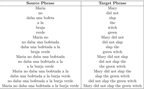
language. Word alignments do not have to be a one-to-one mapping. Words in one language can be aligned to more than one words or no words at all in the other language. Figure 1.1 shows alignment matrix between a Spanish sentence and English sentence. As shown in the example, the English word slapis aligned to three Spanish words daba una bofetada.

Figure 1.1: A sample alignment between a Spanish sentence and English sentence [41] It is not easy to find accurate alignments between words of two languages. Specially, for some function words which may or may not have an equivalent word in the other language. Also, it is important that content words in source language are aligned to the corresponding content word in the target language.

Approaches for learning word alignments can be classified into two general categories, as described by [53], (a) statistical alignment models, and(b) heuristic models. As, statistical alignment models are currently the state of the art, we only focus on them and look at various methods in this category.

In statistical alignment models, we collect statistics from the sentence aligned paral-lel corpus to generate word alignment models. We are given a source language string

f₁J =f1, ..., fj, ..., fJ and a target language string eI1 =e1, ..., ei, ..., eI. In SMT, we have a translation modelP(f₁J|eI₁), which is the translation probability describing the relationship between a source language string and target language string. In this translation model, we introduce a hidden alignment aJ₁ which describes the mapping between word fj and ei. This gives us the statistical alignment model asP(f₁J, aJ₁|eI₁). As shown by [53], the relation between translation model and statistical alignment model is

P(f₁J|eI₁) =∑ aJ

1

(14)

To account for the unknown parameters θ learnt from training data, the statistical alignment model is represented as pθ(f1J, aJ1|e1I). For each sentence pair (fn,en), for n =

1, ..., N, where N is the size of parallel corpus, the alignment is denoted as a=aJ

1. We find

the unknown parameters θ by maximizing the likelihood on the parallel corpus:

ˆ θ= argmax θ N ∏ n=1 ∑ a pθ(fn,a|en) (1.2)

To perform the maximization, Expectation Maximization (EM) [19] or some variant of it is used. After finding the unknown parameters, the best alignment for a pair of sentences can be calculated as:

ˆ

aJ₁ = argmax aJ

1

p_θˆ(f1J, aJ1|eI1) (1.3)

Such statistical alignment models are called generative models and are generally created using unsupervised learning techniques. A major drawback of generative models is that in-corporating arbitrary features is difficult. For example, if we want to include orthographic similarity between two words, presence of the pair in some dictionary, etc. Another draw-back of unsupervised generative models based on EM is that they require large amount of data and processing to converge to a good solution. Discriminative models on the other hand allow us to have arbitrary features. In discriminative models the features do not have to adhere to the independence assumption, that is, features can be dependent on other fea-tures. Whereas, generally in generative EM based algorithms, we assume that the features are independent of each other.

There are various ways to create discriminative models for getting word alignments. Word alignment problem can also be thought of as a maximum weighted matching problem where each pair of words in parallel sentences would be assigned a score depending on how likely they are to be aligned. The word alignment problem can also be considered as a maximum weight bipartite matching problem [63], where nodes correspond to words in the two parallel sentences. Aside from graph matching algorithms, discriminative approaches also use perceptron algorithm [50], support vector machines [14], conditional random fields [6] or neural networks [3].

1.1.2 Translation Model

In phrase-based SMT, continuous sequence of words (phrases) are the atomic units of lation. The source sentence is first broken down into phrases and each phrase is then

(15)

trans-lated. To get the translation of source phrase, a phrase table is learnt from the parallel corpora. [41] states the following advantages of using phrases as atomic units:

• Many-to-many translation can handle non-compositional phrases. • Use of local context in translation.

• Longer phrases can be learnt if more data is available.

The learning of the phrase table can be broken down into three steps:

• Get alignments (as described in Section 1.1.1) of words from parallel corpora in both directions (bi-directional alignments). To combine the alignments from two runs, there are various heuristics in the literature, but for our work, we use the most widely used approach outlined in [43] called grow-diag-final-and. This heuristic has several steps. In the first step, allintersectionalignment points are selected. In thegrow-diag

step, neighbouring and diagonally neighbouring alignment points which are in the union but not in the intersection of the two runs are selected. And, in final-andstep, alignment points which are unaligned and present in theintersectionare selected. For our work, we use GIZA++ [53] to get the bidirectional alignments.

• Using the bidirectional alignments from step 1, extract all possible phrase pairs which are consistent with the alignments [54, 43]. A phrase pair is consistent with the alignments if words within the source phrase are only aligned to words in the target phrase. Table 1.1 shows all the possible phrase pairs that are consistent with the alignments shown in Fig 1.1.

• Assign probabilities to phrase pairs using their relative frequencies:

ϕ( ¯f|¯e) = ∑count(¯e,f¯) ¯ ficount(¯e, ¯ fi) (1.4)

Here, f¯ is a source phrase and e¯ is the target phrase. Along with ϕ( ¯f|¯e), other features likeinverse lexical weighting,direct phrase translation probability and direct lexical weighting are also calculated.

At the end of these steps, we get a phrase table containing the bilingual phrase pairs, the alignments within those phrase pairs and feature scores as shown in table 1.2.

1.1.3 Language Model

The language model is an integral part of an SMT system. The job of a language model is to measure how likely a string of words (sentence) in a language would be uttered by a human speaker, that is, how fluent is the sentence. For example, we have two sen-tences in English, ”this is a house” and ”this a house is”. The language model should

(16)

Source Phrase Target Phrase

Maria Mary

no did not

daba una bofeta slap

a la the

bruja witch

verde green

Maria no Mary did not

no daba una bofetada did not slap

daba una bofetada a la slap the

bruja verde green witch

Maria no daba una bofetada Mary did not slap no daba una bofetada a la did not slap the

a la burja verde the green witch

Maria no daba una bofetada a la Mary did not slap the daba una bofetada a la burja verde slap the green witch no daba una bofetada a la burja verde did not slap the green witch Maria no daba una bofetada a la burja verde Mary did not slap the green witch Table 1.1: All possible phrase pairs consistent with the alignments shown in Fig.1.1

Source Phrase Target Phrase Feature Scores Alignments

in europa in europe 0.829007 0.207955 0.801493 0.492402 0-0 1-1 Table 1.2: A sample entry in the translation model (phrase table)

(17)

tell us that the probability of former sentence should be higher than the latter, that is,

pLM(this is a house) > pLM(this a house is). From this example, we notice that language models along with telling how fluent a sentence is, they also help in deciding the right order of words. They also help in choosing the right words for translation. For example,

pLM(I am going home)> pLM(I am going house).

For an SMT system, the language model is trained on large monolingual corpora of the target language. This is because we want to aid the translation system in deciding a good translation for a source sentence. Due to the abundance of data available in a single language, the amount of training data used in training the language model is generally orders of magnitude more than the parallel corpora used to train the translation model.

The state of the art method to train a language model isn-gram language modelling. In n-gram language models, we compute the probability of a sentenceW =w1, w2, w3, ..., wn. The probability of sentencep(W)can be represented as a joint probability of words in the sentence:

p(W) =p(w1, w2, ..., wn) (1.5)

Using the chain rule, we can break this down:

p(W) =p(w1)p(w2|w1)p(w3|w1, w2)...p(wn|w1, w2, ..., wn−1) (1.6)

Here, we have broken down the probability of a sentence into the probability of words depending on the preceeding words. To be able to calculate these probabilities easily, we limit the history of each word tom words.

p(W) =p(w1)p(w2|w1)p(w3|w1, w2)...p(wn|wn−m, ..., wn−2, wn−1) (1.7)

This model in which we step through a sequence of words and consider a limited history for each transition is called aMarkov chain. Here mis the order of the model. For example, a 3 gram language model would be:

p(W) =p(w1)p(w2|w1)p(w3|w1, w2)p(w4|w2, w3)...p(wn|wn−2, wn−1) (1.8)

To estimate the probability of the n-grams, we collect the required counts from the monolingual corpora and use maximum likelihood estimation:

p(w3|w1, w2) =

count(w1, w2, w3) ∑

wcount(w1, w2, w)

(1.9) Even though we use a large monolingual corpora to train the language model, we still cannot cover every word and its usage. To tackle the problem of unseen words, the literature

(18)

describes various smoothing techniques like add-one smoothing, add-α smoothing, Good-Turing smoothing [26], Witten-Bell smoothing[69], Kneser-Ney smoothing [38], etc.

1.1.4 Decoder

[43] states the mathematical model for translation asp(e|f). The job of the decoder is to find the translation ebest with the highest probability. This can be mathematically formulated as:

ebest=argmaxep(e|f) (1.10)

Figure 1.2: A sample German source sentence broken into possbile phrases and the top four translation options for each of the source phrase [41, p. 159]

When the decoder proposed by [43] has to translate a source sentence, it first breaks the sentence down into the atomic units of phrase-based SMT, that is, phrases as shown in Fig 1.2. The target sentence is then generated left to right in the form of partial translations called hypothesis and it employs a beam search algorithm. The decoder starts with an initial empty hypothesis. A new hypothesis is expanded from an existing hypothesis by selecting the next untranslated source phrase, finding it’s possible target phrase from the translation model. The target phrase is appended to the existing target sentence. The hypothesis is then scored using weighted combination of scores from certain feature functions and the source phrase is marked as translated. The final hypothesis in the search tree which has the highest probability is chosen as the best translation for the source sentence as shown in Fig 1.3

A limitation of this approach is that for each source sentence, an exponential number of hypothesis are generated. Searching through these hypothesis is an NP-complete problem [39]. To tackle this problem, [43] proposed using the hypothesis recombination strategy as in [55]. Along with this, hypotheses are also pruned by comparing their current score and the future score proposed by [43]. Histogram pruning and threshold pruning proposed by [40] are also used to prune the search tree.

(19)

Figure 1.3: A sample German source sentence broken into possbile phrases and the top four translation options for each of the source phrase [41, p. 160]

We mentioned above that the decoder scores each hypothesis using a weighted combi-nation of scores from various feature functions. We also mentioned above that the decoder uses translation model in its process. In addition to the feature scores from the translation model, the decoder also uses the language model we described earlier, a reordering model which is created using the alignments extracted earlier and various feature functions.

[43] proposed a weighted model comprising the phrase translation model (ϕ( ¯f|e¯)), a reordering model (d), and language model (pLM(e)), which is mathematically formulated as: ebest=argmaxe I ∏ i=1 ϕ( ¯fi|e¯i)λϕd(ai−bi1 −1)λd |e| ∏ i=1 pLM(e)λLM (1.11) Hereai andbi1 are the starting and ending position of the source phrase that was translated to the ith target phrase and i−1th target phrase. λϕ, λd and λLM are the weights for translation model, reordering model and language model respectively. These scores are calculated incrementally for each hypothesis.

Such a weighted model is actually a log-linear model of the form:

p(x) =exp

n

∑

i=1

λihi(x) (1.12)

When working with probabilities, it is easier to deal with log values to avoid floating point underflow problems. We can rewrite equation 1.11 as:

p(e, a|f) =exp[λϕ I ∑ i=1 logϕ( ¯fi|e¯i) +λd I ∑ i=1 logd(ai−bi−1−1) +λLM |e| ∑ i logpLM(ei|e1...ei−1)] (1.13)

(20)

This formulation allows us to add more independent feature functions, that is, feature functions that are independent of other feature functions. In practice, Moses [42], a popular SMT toolkit that we use in our work, uses 15 features which are as follows:

• Unknown word penalty (1 feature) • Word penalty (1 feature)

• Phrase penalty (1 feature) • Translation model (4 features) • Lexical reordering (6 features) • Distortion (1 feature)

• Language model (1 feature)

Each of these features have a weight associated with them and it is the job of a tuning algorithm which we will look at in the next section to optimize them.

1.1.5 Tuning

A simple SMT system utilizes number of features during its decoding stage. Each of these features has a weight associated with them, and a default value for each of these weights. To understand which of these features are better indicators of a good translation and vice-versa, we need to tune these weights (also called parameters). While tuning, we need to understand the affect of the parameters on translation performance. A popular metric that is used for this is Bilingual Evaluation Understudy (BLEU) [56]. BLEU compares the output translation with reference translations according to the equation:

BLEUscore =BP ·exp n

∑

i=1

wilog(precisioni) (1.14)

Here, BP is called brevity penalty and is formulated as:

BP = min(1, output−length

reference₋length) (1.15)

wi are the weights associated with different n-gram precisions. These weights are gen-erally set to 1. Brevity penalty is used to penalize phrases that are much shorter compared to the reference translation. A thing to note is that BLEU score is 0 if any of the n-gram precisions is 0. To calculate precision, one simply counts the number of n-grams of system translation which occur in reference translations divided by the total number of n-grams in the system translation. The beauty of this precision based metric is that it allows the

(21)

use of multiple reference translations. Note, reference translations are human generated translations for the source sentence under test.

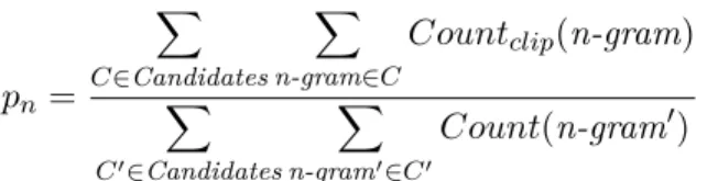
MT systems can easily over-generate reasonable words, which would result in high pre-cision for sentences like the one in example 1.4. To counter this issue, modified n-gram precision exhausts a reference n-gram once it is matched, that is, a reference n-gram once matched cannot be matched again. Fig. 1.4 also shows the output of modified n-gram precision.

System Translation: the the the the the the the. Reference 1: The cat is on the mat.

Reference 2: There is a cat on the mat. Modified unigram precision: 2

7.

Figure 1.4: An example of modified n-gram precision. Modified n-gram precision is given as follows:

pn=

∑

C∈Candidates ∑ n-gram∈C

Countclip(n-gram)

∑

C′∈Candidates ∑ n-gram′_∈C′

Count(n-gram′) (1.16)

Candidates refers to the target set of sentences. Where, Countclip =min(Count,

M ax_Ref_Count), that is, do not exceed the largest count of the n-gram in any single reference.

When tuning the parameters of the feature functions, we always use a small parallel corpora that was not used during the training of the models. This small parallel corpora is called the tuning set or dev set. Tuning algorithms can be divided into two main classes:

• Batch tuning algorithms: In batch tuning algorithms, the complete tuning set is decoded with some initial weights. Generally an n-best list of decoded output is generated. The tuning algorithm then updates the weights based on the decoder output. The tuning set is again decoded based on the updated weights. This procedure is repeated to optimize the weights until we reach convergence or up to a certain number of iterations. Various such tuning algorithms have been described in the literature, Minimum Error Rate Training (MERT) [53] is the most widely used tuning algorithm. Lattice MERT [45] is a variant of MERT that uses lattices instead of n-best list. Pairwise ranked optimization (PRO) [32] works by ranking learning the weight set that ranks the n-best list in the same order as BLEU. Batch MIRA [13] is a type of margin based classification algorithm that works in the batch tuning setting. • Online tuning algorithms: Online algorithms work together tightly with the decoder.

(22)

next sentence is decoded. The MIRA tuning algorithm [13] is the most widely used tuning algorithm in this setting.

1.2 Bi-LMs and why do we need them?

In phrase-based SMT, during the decoding process, the decoder decodes a partial hypothesis containing a phrase from the source sentence into the target language. During this process, it has very little information from source words outside the current phrase pair. [61] states that information from source words outside the current phrase pair is incorporated only indirectly, via target words that are translations of these source words, if the relevant target words are close enough to the current target word to affect the language model scores. To add more information about the source words, [51] introduced part-of-speech basedbilingual language models (Bi-LMs) which were extended by [61]. Bilingual language models are generated by aligning each target word in the parallel training corpus with source words to create bitokens. These bitokens are then used to estimate an n-gram language model. Coarse Bi-LMs are Bi-LMs which are estimated by first clustering the bitokens and then estimating the language model. Similarly, coarse LMs are also language models which are estimated by clustering the words and then estimating the language model based on the clustered data. [51] generated the Bi-LMs by first replacing the words in the parallel corpus with part-of-speech tags. Using this augmented corpus and alignments, the bitokens were created to estimate the Bi-LMs. Similarly, [61] used MKCLS [52] to create word classes.

In this thesis, we propose a new method of generating Bi-LMs. We create word em-beddings and bilingual word emem-beddings (Chapter 2 will give an introduction to word embeddings and bilingual word embeddings) of words in our training data. These embed-dings are clustered using a spectral clustering algorithm. This allows us to group together words which are semantically similar. These clusters are used to augment the original cor-pus, hence reducing the vocabulary of the original parallel training corpus. The augmented corpora are used to training Coarse LMs and Bi-LMs (Chapter 3 explains in detail the steps to create Coarse LMs and Bi-LMs). We call these LMs & Bi-LMs coarse because they are estimated using data whose vocabulary has been reduced by using certain clusters. In the literature, work has been done to use part-of-speech tags or monolingual clusters of words using Brown clustering algorithm [9].

In our work we propose three new approaches of creating and using coarse LMs and Bi-LMs to improve statistical machine translation task. We show that our best approach which was based on our original hypothesis of using bilingual word embeddings and monolingual word embeddings achieves+1.4 BLEU pointsin the Chinese-English SMT task and two of our approaches achieve an increment in BLEU score by0.1and 0.4.

(23)

1.3 Summary

In this chapter we introduce the individual steps in training a statistical machine translation system. We then give an introduction to bilingual language models and how they can be helpful in statistical machine translation. In the end we introduce our idea of learning bilingual language models using word embeddings. In Chapter 2 we will discuss about word embeddings, bilingual word embeddings and a method to judge the best bilingual word embeddings. In Chapter 3, we will discuss in detail about bilingual language models. We will also introduce our baseline system and our approaches to develop bilingual language models. Later, in Chapter 4 we describe our experimental setup and results from our approaches. Finally, in Chapter 5 we conclude this thesis and introduce ideas that would be natural extensions of our work which we would like to do in the future.

(24)

Chapter 2

Word Embeddings

2.1 What are word embeddings?

Semantic relations between words denote how two words are related or how close their meanings are. One way to represent this relation is by representing each word as a vector (also called word embeddings) such that, words which are similar, their vectors would lie closer to each other in somendimension space. Whereas, vectors of dissimilar words would lie far apart. When creating the word embeddings, we assume that words are characterized by the words that surround it, that is the company that the word keeps [28]. The relation between two vectors (words) is represented by using a displacement vector, that is, a vector between two vectors. The displacement vector can help us find relations likequeen:king ::

woman:man, which would mathematically be denoted as vqueen−vking =vwoman−vman. Here,vi means ann-dimension vector of the word i.

Learning word embeddings broadly falls into two categories. Clustering based repre-sentations, often use hierarchical clustering methods to group similar words based on their contexts. Brown Clustering [9] and [57] are the two most dominant approaches. Hidden Markov Models can also be used to induce clustering on words [36]. The problem with clustering approach is that the representations generated are sparse vectors. The reason they are sparse is because the vectors generated would generally be one-hot vectors. Such vectors are contains binary values 0 or 1 where 1 indicates the cluster number to which the word belongs. To reduce the sparsity issues, the other approach is to generate dense representations of words. These representations are low dimensional real valued dense vec-tors. These embeddings can be generated by using latent semantic analysis [18], canonical correlation analysis [21], neural-networks [16, 35, 47, 49, 27].

As estimating Bi-LMs required parallel corpora of two languages, it is natural to utilize bilingual word embeddings that denote semantic relations among words across two lan-guages, that is words which are semantically similar in either of the languages are close to each other in somen-dimension space. This enables us to understand how close a word in

(25)

one language would be to another word in the second language. For example, the English wordlakeand Chinese word潭(deep pond), even though they are not direct translations of each other, but due to their semantic similarity, they would be close to each other in some

n-dimension space. And words which are semantically similar to潭 (deep pond) and possi-bly direct translations oflake would also be close to each other in thatn-dimension space. For word embeddings, we measure semantic similarity by measuring the cosine similarity between two word embeddings. It is formally defined as:

similarity=cos(θ) = A.B ||A_||||B_|| = ∑_n i=1AiBi √∑n i=1A2i √∑n i=1B2i (2.1)

Here, Aand B are two vectors of sizen.

Bilingual word embeddings have been created by using various techniques like latent dirichlet allocation and latent semantic analysis [8, 71], canonical correlation analysis [24], neural-networks [37, 73, 48, 31, 12]. In the next section we discuss the reasons for choosing the algorithms to create monolingual and bilingual word embeddings.

2.2 Creating Word Embeddings

As stated in Section 2.1, the underlying idea of most of the methods is based on the concept that the meaning of a word can be determined by the company that it keeps. This idea is the underlying method for most of the work done to create monolingual and bilingual word embeddings. For both the embeddings, most of the popular approaches are based on using either canonical correlation analysis [21, 24] and neural networks [16, 35, 37, 47, 49, 48, 73, 31, 12]. Neural network approaches to create word embeddings have been widely adopted due to the following advantages:

• Training the networks can be done using parallel processing and distributed process-ing.1

• Graphical processing units (GPU) can be utilized for faster training.2

• If new data is available for training, the weights of the network can be updated by only using the new data and not the previously used training data. That is, the network does not need to be retrained by using all the previous and new training data. Matrix factorization methods like canonical correlation analysis and latent semantic analysis would require retraining of models using all the data.31

1_{Gensim toolkit[58] has implementation of word2vec[47] that allows training of word embeddings using}

parallel processing. It also allows updating of network weights with new training data that was not used to train the network previously.

(26)

• They are currently state of the art methods in producing good quality word embed-dings.

Due to their speed of training and being the state of the art algorithms for training embeddings, we decided to use a neural network based approach. For creating monolingual word embeddings we utilize Word2Vec [47, 49, 48], as it is currently state of the art toolkit for creating monolingual word embeddings. We will explain the usage of monolingual embeddings in Chapter 3.

For creating bilingual word embeddings, [73] utilize sentence aligned parallel corpus and their alignments to induce the embeddings whereas [31] only utilizes a sentence aligned par-allel corpus (they state that there is no theoretical dependence on sentence aligned parpar-allel corpora and technically it could also be used with document aligned parallel corpora). As creating alignments is not perfect and they have a small margin of error (the state of the art method to create alignments [4] for Chinese-English parallel corpus has an alignment error rate of 30%), using word embeddings that require alignments [73] would increase the chances of propagating errors. Hence, to keep the possibility of errors in creating alignments and creating bilingual word embedding independent of each other, we use the work of [31] to create the bilingual word embeddings.

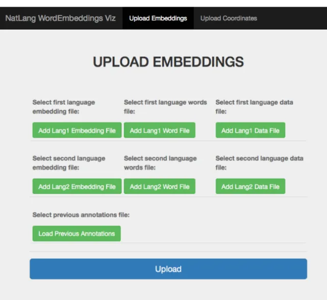
When training bilingual word embeddings we need to manually choose multiple hyper-parameters for the algorithms. Varying the hyper-hyper-parameters changes the embeddings that are generated. To understand the effects of the hyper-parameters and to choose the ones which give good embeddings we introduce WordEmbeddingsViz4, a tool to visualize bilingual word embeddings and to study the effects of different values of hyper-parameters. In the next section we explain how one can use WordEmbeddingsViz to choose the best embedding parameters.

2.3 Visualizing Word Embeddings

WordEmbeddingsViz enables a user to visualize bilingual word embeddings. The tool uses t-Distributed Stochastic Neighbor Embedding (t-SNE) [67] to project the embeddings into two dimension space. SNE is a non linear dimensionality reduction technique. t-SNE constructs a probability distribution over pairs of objects in high dimensions such that similar objects (that is, objects which are close to each other) have a high probability whereas dissimilar objects (objects that are far apart) have a low probability. t-SNE defines a similar probability distribution over pairs of objects in lower dimensions and minimizes the Kullback-Leibler divergence between the two distributions. In the higher dimension space, it uses Gaussian distribution to measure the similarity between objects, whereas in lower dimension space, it uses a Student’s t-distribution to measure the similarity. This is because 4_{WordEmbeddingsViz: Tool to visualize bilingual word embeddings}_{https://github.com/sfu-natlang/}

(27)

Student’s t-distribution has a long tail and it allows dissimilar objects to be modeled far apart. [67] showed that due to t-SNE’s non-linear dimensionality reduction and optimization function, it handles the modeling of curved manifolds better than other techniques like Classical Scaling [65] and Sammon Mapping [60]. t-SNE produces better visualization than other techniques by reducing the tendency to crowd points together towards the center of the map. Techniques like Isomap [64] and Locally Linear Embedding [59] are prone to this problem

To use visualize the embeddings, a user will upload the following for each language: • Word Embeddings

• Words

• Training Corpus (with part-of-speech for one language) • Alignments (optional)

Figure 2.1 shows the upload screen where a user can upload the required data.

We require part-of-speech (POS) for one of the languages as this will be used by the tool to show a list of the top 1000 words by their occurrence count for verb, noun, adjective & adverbPOS tags. For our work, we extracted POS tags for English data using the Stanford POS tagger [66].

WordEmbeddingsViz will perform non-linear dimensionality reduction using tSNE on the word embeddings. The dimensions would be reduced to two dimensions. The value of these dimensions for each word would be treated as x and y coordinates to visualize them as a scatter plot. Figure 2.2 shows the scatter plot for bilingual word embeddings of Chinese(Zh)-English(En) parallel corpus. The user can then zoom into the scatter plot to look at the word embeddings. The user can also select one of the English words from the sidebar (sidebar shows a list of top 1000 for each of the verbs, nouns, adjectives and adverbs). On selection of a word from the sidebar, that word will be highlighted and the user can then zoom in to look at the neighbouring embeddings. If for any English word, there are one or more Chinese words in the neighbourhood that are possible translations of that English word, then the user can align them using the alignment option built into the tool. Figure 2.3 and Figure 2.4 shows examples of alignments between English words

broadcast, braodcast (an incorrect spelling of broadcast in the corpus)& broadcasting, and, clocks, timepiece & chimingalong with their Chinese counterparts. The alignments can also be downloaded which can then be utilized for various usecases, such as, using the annotated alignments as information in word alignment algorithms.

Using WordEmbeddingsViz, a human annotator can look at bilingual word embed-dings generated with different parameters. If the embedembed-dings generated are of good quality then semantically similar words in two languages would lie close to each other in the pro-jected space.

(28)

Figure 2.1: WordEmbeddingsViz upload screen: Here, the user can upload bilingual word embeddings, word list, training corpus and alignments (optional)

(29)

Figure 2.2: WordEmbeddingsViz: A scatter plot of word embeddings of Zh-En parallel corpus. Orange squares represent English words and blue circles represent Chinese words.

Figure 2.3: WordEmbeddingsViz: Alignments of English wordsbroadcast, braodcast, broad-casting with their Chinese counterparts.

(30)

Figure 2.4: WordEmbeddingsViz: Alignments of English wordsclocks, timepiece & chiming

with their Chinese counterparts.

2.4 Summary

In this chapter we introduced word embeddings and bilingual word embeddings. We also described a tool WordEmbeddingsViz, which we developed to judge the bilingual word embeddings. In the next chapter, we will provide an in depth description of bilingual language models and our approach of using word embeddings to model bilingual language models.

(31)

Chapter 3

Bilingual Language Models

In phrase-based statistical machine translation (SMT), the decoder (Section 1.1.4) breaks down a source sentence into phrases and translates one source phrase at a time. For each source phrase, the decoder uses a translation model (Section 1.1.2) to get the correspond-ing target phrase. To model the target language fluency, it also uses a language model (Section 1.1.3). A log-linear combination of these models along with additional features are used to score each hypothesis. The decoder then searches for a path in the search tree which gives the highest hypothesis score for the final translation.

As stated in section 1.2, during the decoding process, information from source words outside the current phrase pair in consideration is available indirectly through target words which are translations of these source words, if those target words are close enough to affect the language model scores. Due to this, the translation of each source phrase is performed in isolation without significant information from other source words in the sentence. The effect can be seen in the sentence Maria no daba una bofetada a la burja verde. For this sentence we would get the following phrase segmentations: Maria no, daba una bofetada a la, bruja verde. Here, the translation of Maria nois not affected by the source words daba

orbofetadaorbruja. The other possible segmentation could be as shown in Table 1.2. The translation of wordsMaria no daba una bofetada a lacan be done using the phrases Maria no, daba una bofetada a laorMaria, no, daba una bofetada, a la. The decoder cannot make use of the fact that both these options lead to the same translationMary did not slap the. If the first option is chosen, the translation of no is affected by Maria, but in the second option,nois only affected by Maria via the language model.

To introduce the effect of source words outside the current phrase pair in consideration, a considerable amount of work has been done in the past. In this thesis, we extend the work of [61] to create bilingual language models (Bi-LMs) that will be used as additional features to the decoder.

(32)

3.1 What are Bilingual Language Models?

Bi-LMs are n-gram language models which are trained on bitokens instead of simple word tokens as done for standard language models (Section 1.1.3). Bitokens are generated us-ing the source and target sentences from the parallel corpora and their alignments. To understand what bitokens are, let us look at two parallel sentences shown in Fig. 3.1:

Target: nous nous devions d’ être progressistes

Source: we had to be very forward looking

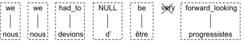
Figure 3.1: Source and target sentences with their alignments for creating bitokens [61] Using the parallel sentences and their alignments shown in Fig. 3.1 we will create a bitoken sequence. When creating the bitokens, we want to make sure that all the target words are used. In the example above, the source wordwe is aligned to target words nous nous. We will replicatewetwice and align bothnouswith both theweto create the bitokens

we-nous and we-nous. Next we have the source words had to aligned todevions. We will join had and to to create a single token had_to and align that to devions to get had_to-devions. Since, the target wordd’ is not aligned to any source word, we align it to NULL

and create a bitoken NULL-d’. For the source wordvery, as it is not aligned to any target word, it is dropped. Similarly, we also get the bitokenforward_looking-progressistes. The final bitokens are shown in Fig. 3.2:

we nous we nous had_to devions NULL d’ be être very forward_looking progressistes

Figure 3.2: Bitokens created from the parallel sentences and their alignments shown in Fig. 3.1

More formaly, given a pair of sentences eI₁ = e1...eI, f1J = f1...fJ and alignments

A={(i, j)}, the bitokens are:

bj ={fj} ∪ {ei|(i, j)∈A} (3.1) This makes sure that the number of bitokens bj are equal to the number of target words. These bitoken sequences can then be used to create a language model called a bilingual language model, formalized as follows:

(33)

Number of Target Word Types Number of Bitoken Types

152318 3827728

Table 3.1: Number of target words vs. number of bitokens in our data

p(eI₁, f₁J, A) = J

∏

j=1

P(bj|bj−1...bj−n) (3.2)

The advantage of using Bi-LMs is that they can be used in phrase-based SMT as ad-ditional features in the log linear model. When the decoder scores each hypothesis using scores from translation and language model, it can easily incorporate the probability from Eqn. 3.2. Even though, Bi-LMs are language models, but they act more as translation models as they do not model the fluency of the target language but model the translation of source words.

In Bi-LMs the bitoken vocabulary size increases by many folds compared to the vocab-ulary size of target words. For example, as shown by [61], the target word être might be split into multiple bitokens: be-être, being-être and to_be-être. This large vocabulary also leads to an increase in the sparsity in data for language modelling. Table 3.1 shows the number of bitokens compared to the number of target words in our corpus. We will explain in detail about our data and alignments used to create the bitokens in Chapter 4.

To tackle the problem of large vocabulary and sparsity, [51] introduced coarse Bi-LMs. When training LMs and Bi-LMs, if the words are replaced by some word class to reduce the vocabulary size, they are then calledCoarse LMs/Bi-LMs. When creating Bi-LMs, [51] replaced both the source and target words in their Arabic-English SMT with the corre-sponding Part-of-Speech tags. [61] extended this idea and replaced both source and target words with cluster ids generated usingmkcls[52]. [61] not only clustered the initial source and target words, but also experimented with clustering the bitokens too. Figure 3.3 shows the 3 ways of creating coarse bitoken sequences for Coarse Bi-LMs:

• Word Clustering: Create bitoken sequences with only source and target word cluster ids. The bitokens are then used to create Bi-LMs.

• Bitoken Clustering 1: Create bitokens without clustering source and target words. Cluster the bitokens and then use the bitoken sequences augmented with bitoken cluster ids to create Bi-LMs.

• Bitoken Clustering 2: Create bitoken sequences with source and target word cluster ids. Cluster the bitoken sequences and then use the bitoken sequences with bitoken cluster ids to create Bi-LMs.

(34)

we nous we nous had_to devions NULL d’ be être very forward_looking progressistes Target: nous nous devions d’ être progressistes Source: we had to be very forward looking

Bitoken Sequence E1 F1 E1 F1 E2_E3 F2 NULL F3 E2 F4 E4_E4 F5 Word Clustering E1 F1 E1 F1 E2_E3 F2 NULL F3 E2 F4 E4_E4 F5 Bitoken Clustering 2 B1 B1 B3 B3 B4 B5 Bitoken Clustering 1 B1 B1 B3 B3 B4 B5 we nous we nous had_to devions NULL d’ be être forward_looking progressistes

Figure 3.3: Creating bitokens, word clusters and bitoken clusters [61]

[2, 5] showed that coarse LMs along with the standard LM are particularly effective for morphologically rich languages. Motivated by this, [61] used a combination of coarse LMs and coarse Bi-LMs in their experiments. They created the following four feature functions: • Brown Coarse LM 100: Using mkcls (Brown clustering), the target corpus is clustered into 100 clusters. The words in the original target corpus are replaced by their respective cluster ids. This step brings down the vocabulary of the original target corpus to 100. Hence, the new augmented corpus is calledcoarse target corpus.

Using this coarse corpus, a language model is then trained called Brown Coarse LM 100, where 100 denotes the vocabulary size of the corpus used to train the language model. (See Fig. 3.6)

• Brown Coarse LM 1600: Similar to Brown Coarse LM 100, the target corpus is clustered into 1600 clusters using mkcls. The original corpus is then augmented with the new cluster ids of the respective words to create a coarse target corpus. This coarse target corpus is used to train the language modelBrown Coarse LM 1600. (See Fig. 3.5)

• Brown Coarse Bi-LM (400, 400): Usingmkclsfirst cluster the source and target parallel corpus into clusters of size 400 and 400 respectively. The words in the original parallel corpus are then replaced with their corresponding cluster ids to create coarse

(35)

Target Corpus 100 Clusters using Brown Clustering Coarse Target Corpus Brown Coarse LM 100

Figure 3.4: Creating Brown Coarse LM 100 [61] Target Corpus 1600 Clusters using Brown Clustering Coarse Target Corpus: 1600 Brown Coarse LM 1600

Figure 3.5: Creating Brown Coarse LM 1600 [61]

source and target corpora. Using the coarse corpora and the alignments between the words in the original parallel corpus, bitokens sequences are generated using the process shown in Fig. 3.2. The bitoken sequences are then used to estimate a language model Brown Coarse Bi-LM (400, 400). (See Fig. 3.4)

• Brown-Brown Coarse Bi-LM (400, 400): To further reduce the vocabulary of bitokens created in the previous step, they are clustered into 400 clusters usingmkcls. The bitokens in the bitoken sequences are replaced with their corresponding cluster ids to createcoarse bitoken sequences. The coarse bitoken sequences have a reduced vocabulary of 400 and they are used to estimate the language model Brown-Brown Coarse Bi-LM 400(400, 400). (See Fig. 3.7)

Apart from the above mentioned cluster sizes, [61] also experimented with other cluster sizes and combinations but they showed that the above combination performs well for multiple language pairs.

In this thesis we extend the work of [61] to improve coarse LMs and Bi-LMs. In the next section, we describe in detail the contribution of this thesis, that is, using word embeddings to improve coarse LMs and Bi-LMs.

3.2 Bi-LMs using Word Embeddings

mkcls [52] is one of the most widely used word clustering toolkits. Motivated by Brown Clustering [9], mkcls1 _{implements an ensemble of optimzers and merges their results to} cluster words into the provided number of classes. mkcls can only cluster monolingual corpus and it performes strongly in that aspect [7].

1_{Understanding} _mkcls _by _Dr. _Chris _Dyer: _{http://statmt.blogspot.ca/2014/07/}

(36)

Target Corpus Source Corpus Coarse Target Corpus Coarse Source Corpus HMM and IBM Model 2 Alignments Bitoken Sequences Brown Coarse Bi-LM (400, 400) 400 Clusters using Brown Clustering 400 Clusters using Brown Clustering

Figure 3.6: Creating Brown Coarse Bi-LM (400, 400) [61] Bitoken Sequences 400 Clusters using Brown Clustering Coarse Bitoken Sequences Brown-Brown Coarse Bi-LM 400 (400, 400)

Figure 3.7: Creating Brown-Brown Coarse Bi-LM (400, 400). It uses the bitoken sequences created in Fig 3.4 [61]

The main goal of Bi-LMs is to add more information about source words that are not in the current phrase pair. But current state of the art coarse Bi-LMs only depend on alignments and monolingual word clusters to add more information about source words. For example, the English wordlakeand Chinese word 潭(deep pond), which are not direct translations of each other, won’t be captured by alignments and hence won’t be influencing the coarse Bi-LMs until unlessmkclsassigns潭and another Chinese word which is a direct translation of lake to the same cluster. To increase the probability that words in Chinese which are semantically similar to lakeand possibly direct translations get clubbed together in a cluster, we utilize bilingual word embeddings to create the coarse Bi-LMs.

3.2.1 Using Word Embeddings to create Bi-LMs

In Chapter 2, we mention that we utilize [31] to create bilingual word embeddings for the words in our sentence aligned parallel corpus. To create coarse LMs and Bi-LMs, as done by [61], we need to cluster these embeddings. As mentioned earlier, in our baseline system, we usedmkclsto cluster the words in our parallel corpus. To cluster word embeddings, we used greedo [62], a bottom-up hierarchical clustering algorithm for clustering low-dimensional representation of words under the [9] model. [62] show that the clusters created bygreedo recover clusters which are of comparable quality to the algorithm of [9]. Using greedo gives us the opportunity to compare our approach to the baseline system without any modifications to the number of clusters because mkclsalso creates Brown clusters.

(37)

To use the embeddings and their clusters for creating coarse LMs and coarse Bi-LMs, we propose the following six new feature functions:

• Embed Coarse LM 100 and Embed Coarse LM 1600 The target word embed-dings from the bilingual word embedembed-dings are clustered into clusters of size 100 and 1600. We create two copies of the target corpus. In the first copy, we replace the target words with their cluster ids from 100 clusters to create coarse target corpus 100. Similarly, in the other copy of the target corpus, we replace the target words with their corresponding cluster ids from 1600 clusters to create acoarse target corpus 1600. The two coarse target corpora are then used to estimate coarse language models

Embed Coarse LM 100 andEmbed Coarse LM 1600.

• Embed Coarse Bi-LM (400, 400)The target word embeddings from the bilingual word embeddings are clustered into 400 clusters and similarly the source word embed-dings are clustered into 400 clusters. The target words in the target corpus are then replaced with the cluster ids from 400 target word clusters to create a coarse target corpusand similarly the source words in the source corpus are replaced with their cor-responding cluster ids to create corase source corpus. The two coarse corpora along with bidirectional word alignments between the words in the original parallel corpus are used to create bitoken sequences using the process shown in Fig. 3.2. These bito-ken sequences are then used to estimate a coarse Bi-LMEmbed Coarse Bi-LM (400, 400).

• Embed-Brown Coarse Bi-LM 400(400, 400) In this feature function we use the bitoken sequences created in the previous step. The bitokens are clusterd into 400 clusters using mkcls. The bitokens in the bitoken sequences are then replaced with their corresponding cluster ids to create coarse bitoken sequences. These coarse bitokens sequences are used to estimate coarse Bi-LM Embed-Brown Coarse Bi-LM 400(400, 400).

• Embed-Embed Coarse Bi-LM 400(400, 400) Similar to the previous step, we use the bitoken sequences that we had created earlier. Instead of clustering them using mkcls, we create bitoken embeddings of the bitokens using word2vec. These bitoken embeddings are clustered into 400 clusters using greedo. The bitokens in the bitoken sequences are then replaced with their corresponding cluster ids to create

coarse bitoken sequences. These coarse bitokens sequences are then used to estimate the coarse Bi-LM Embed-Embed Coarse Bi-LM 400(400, 400).

• Embed-Embed Coarse Bi-LM 400(|Vf|, |Ve|) In this feature function, instead of first reducing the vocabulary of the parallel corpus, we will use the full vocabulary to create the bitokens. To do this, we take the parallel corpus and the bidirectional

(38)

Target Corpus Source Corpus 100 Clusters of Target Words using Stratos et al, 2014 Coarse Target Corpus Coarse Target Corpus Embed Coarse LM 100 Embed Coarse LM 1600

Bilingual Word Embeddings using Hermann and Blunsom, 2014

1600 Clusters of Target Words using Stratos et

al, 2014

Figure 3.8: Creating Embed Coarse LM 100 and Embed Coarse LM 1600

Coarse Target Corpus Coarse Source Corpus HMM and IBM Model 2 Alignments Bitoken Sequences Embed Coarse Bi-LM (400, 400) Target Corpus Source Corpus 400 Clusters of Target Words using Stratos et al., 2014

Bilingual Word Embeddings using Hermann and Blunsom, 2014

400 Clusters of Source Words using Stratos et

al., 2014

Figure 3.9: Creating Embed Coarse Bi-LM (400, 400)

alignments to create the bitoken sequences using the process shown in Fig. 3.2. Using word2vec bitoken embeddings are generated for the bitokens. These bitokens em-beddings are clustered into 400 clusters using greedo. The bitokens in the bitoken sequences are replaced with their corresponding cluster ids to generatecoarse bitokens sequences. These coarse bitoken sequences are further used to estimate coarse Bi-LM

Embed-Embed Coarse Bi-LM 400(_|V_f_|, _|V_e_|). Here, Vf denotes the full vocabulary of the source corpus andVe denotes the full vocabulary of the target corpus.

We propose three new SMT systems Embed-Brown, Embed-Embed-Reduced-Vocab and

Embed-Embed-Full-Vocab that use a combination of the newly proposed feature functions. Table 3.2 shows the combination of feature functions used in the baseline and the three new systems. All the three systems that have been emphasized in the table utilize bilingual word embeddings when creating Coarse LMs and Bi-LMs.

(39)

Bitoken Sequences 400 Clusters using Brown Clustering Coarse Bitoken Sequences Embed-Brown Coarse Bi-LM 400 (400, 400)

Figure 3.10: Creating Embed-Brown Coarse Bi-LM 400(400, 400) Bitoken Sequences 400 Clusters using Stratos et al., 2014 Coarse Bitoken Sequences Embed-Embed Coarse Bi-LM 400 (400, 400) Embeddings of Bitokens using Mikolov

et al., 2013

Figure 3.11: Creating Embed-Embed Coarse Bi-LM 400(400, 400) SMT System Feature Function 1 Feature Function 2 Feature Function 3 Feature Function 4 Baseline Brown Coarse

LM 100 Brown Coarse LM 1600 Brown Coarse Bi-LM (400, 400) Brown-Brown Coarse Bi-LM 400(400, 400) Embed-Brown Embed Coarse LM 100 Embed Coarse LM 1600 Embed Coarse Bi-LM (400, 400) Embed-Brown Coarse Bi-LM 400(400, 400) Embed- Reduced-Vocab Embed Coarse LM 100 Embed Coarse LM 1600 Embed Coarse Bi-LM (400, 400) Embed-Embed Coarse Bi-LM 400(400, 400) Embed- Embed-Full-Vocab Embed Coarse LM 100 Embed Coarse LM 1600 - Embed-Embed Coarse Bi-LM 400(|Vf|,|Ve|) Table 3.2: Feature combinations used in Baseline, Embed-Brown, Embed-Embed-Reduced-Vocab and Embed-Embed-Full-Embed-Embed-Reduced-Vocab SMT systems.

(40)

Target Corpus Source Corpus HMM and IBM Model 2 Alignments Bitoken Sequences Embed-Embed Coarse Bi-LM 400(|V_f|, |V_e|) 400 Clusters using Stratos et al., 2014 Coarse Bitoken Sequences Embeddings of Bitokens using Mikolov

et al., 2013

Figure 3.12: Creating Embed-Embed Coarse Bi-LM 400(_|V_f_|, _|Ve|)

The feature functions in each of the system in Table 3.2 are added to the log linear model (Eqn. 1.13) as follows: