STAT 503X Case Study 2: Italian Olive Oils
1
Description
This data consists of the percentage composition of 8 fatty acids (palmitic, palmitoleic, stearic, oleic, linoleic, linolenic, arachidic, eicosenoic) found in the lipid fraction of 572 Italian olive oils. (An analysis of this data is given in (Forina, Armanino, Lanteri & Tiscornia 1983)). There are 9 collection areas, 4 from southern Italy (North and South Apulia, Calabria, Sicily), two from Sardinia (Inland and Coastal) and 3 from northern Italy (Umbria, East and West Liguria).
The data available are:
Region South, North or Sardinia
Area Sub-regions within the larger regions (North and South Apulia, Calabria, Sicily, Inland and Coastal Sardinia, Umbria, East and West Liguria
Palmitic Acid Percentage×100 in sample Palmitoleic Acid Percentage×100 in sample Stearic Acid Percentage×100 in sample Oleic Acid Percentage×100 in sample Linoleic Acid Percentage×100 in sample Linolenic Acid Percentage×100 in sample Arachidic Acid Percentage×100 in sample Eicosenoic Acid Percentage×100 in sample
The primary question is “How do we distinguish the oils from different regions and areas in Italy based on their combinations of the fatty acids?”
2
Suggested Approaches
Approach Reason Type of questions addressed Data Restructuring This is very clean data so I don’t see
any need to restructure.
Summary Statistics To get at location and scale informa-tion for each variable, and by groups
What is the average percent compo-sition of eicosenoic acid overall? Is there a difference in the average per-centage of eicosenoic acid for olives from different growing regions? Visual InspectionThe
aim of visual methods is to understand sep-arations, help decide the best classification method, and hence interpret solutions
Univariate Plots, Bivariate Plots, Touring Plots
Are there differences in the fatty acid composition between the olives from different growing regions?
Numerical Analysis The aim of numerical solutions is to get the best predictive results.
Linear Discriminant Analysis (LDA), Quadratic Discriminant Analysis (QDA), Classification and Regression Trees (CART), Forests, Feed-Forward Neural Networks and Support Vector Machines
“Can define the percentage com-position of fatty acids that distin-guishes olives from different growing regions?”
3
Actual Approaches
3.1
Summary Statistics
The following tables contain information on the minimum, maximum, median, mean and standard deviation for the fatty acids, in total and broken down by different growing region.
All the 572 observations (values reported as percentages):
palmitic palmitoleic stearic oleic linoleic linolenic arachidic eicosenoic
Min. 6.10 0.15 1.52 63.00 4.48 0.00 0.0 0.01
Median 12.01 1.10 2.23 73.02 10.30 0.33 0.61 0.17
Max. 17.53 2.80 3.75 84.10 14.70 0.74 1.05 0.58
Mean 12.32 1.26 2.29 73.12 9.81 0.32 0.58 0.16
Std. Dev. 1.69 0.53 0.37 4.06 2.43 0.13 0.22 0.14
From the summary statistics we notice that olive oils are mostly constituted of oleic acid. Palmitic accounts for about 12% on average and the rest less than 10% on average.
n palmitic palmitoleic stearic oleic linoleic linolenic arachidic eicosenoic
South 323 13.32 1.55 2.29 71.00 10.33 0.38 0.63 0.27 Sardinia 98 11.11 0.97 2.26 72.68 11.97 0.27 0.73 0.02 North 151 10.95 0.84 2.31 77.93 7.27 0.22 0.38 0.02 Nth Apul 25 10.27 0.62 2.35 78.20 7.06 0.43 0.72 0.35 Calabria 56 13.02 1.21 2.63 73.07 8.19 0.46 0.64 0.28 Sth Apul 206 13.96 1.84 2.11 69.11 11.66 0.35 0.60 0.24 Sicily 36 12.3 1.05 2.74 73.58 8.35 0.42 0.76 0.38 Inla Sard 65 10.98 0.95 2.17 73.61 11.25 0.29 0.74 0.02 Coas Sard 33 11.38 1.01 2.44 70.86 13.37 0.24 0.72 0.02 East Lig 50 11.45 0.84 2.41 77.46 6.89 0.26 0.64 0.02 West Lig 50 10.3 1.08 2.57 76.74 8.97 0.05 0.07 0.02 Umbria 51 10.86 0.60 1.94 79.56 5.97 0.34 0.42 0.02
Southern oils have much higher eicosenoic acid on average eicosenoic and slightly higher palmitic and palmitoleic acid content. The north and sardinian oils have some difference in the average oleic, linoleic and arachidic acids.
Among the southern oils there is some difference in most of the averages. Northern oils have some difference in most of the averages.
3.2
Visual Inspection
The objective here is to find differences in the measured variables amongst the classes. Differences here might be actual separations between classes on a variable or linear combination of variables. The approach is relatively simple:
1. Use color and or symbol to code the categorical class information into plot.
2. Begin with low-dimensional plots (histogram, density plot, dot plot, scatterplot) of the measured vari-ables and work up to high-dimensional plots (parallel coordinate plot, tours), exploring class structure in relation to data space.
3.2.1 Regions - Univariate Plots
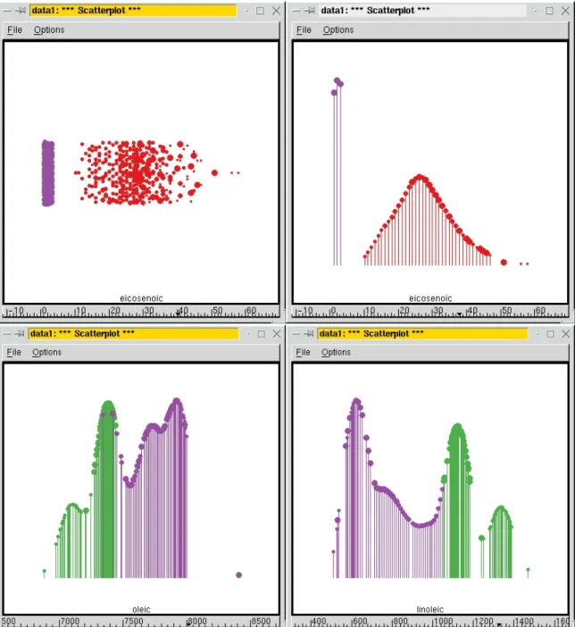
Using 1D Plot mode sequentially work through the variables, either by manually sepecting variables or cycling through automatically, to examine separations between regions. Its possible to neatly separate the oils from southern Italy from the other two regions using just one variable, eicosenoic acid. Figure 1 displays a textured dotplot and an ASH plot of this variable.
The oils from southern Italy are removed, and we concentrate on separating the oils from northern Italy and Sardinia. Although a clear separation between these two regions cannot be found using one variable, two of the variables, oleic and linoleic acid, appear to be important for the separation (Figure 1).
3.2.2 Regions - Bivariate Plots
Starting from the two variables identified by the univariate plots as important for separating northern Italian oils from Sardinian oils, the remaining variables are explored in relation two these two using scatterplots. Oleic acid and linoleic acid show some, but not cleanly, separated regions. Arachidic acid and linoleic acid display a clear separation between the regions, but it is a very non-linear boundary.
3.2.3 Regions - Multivariate Plots
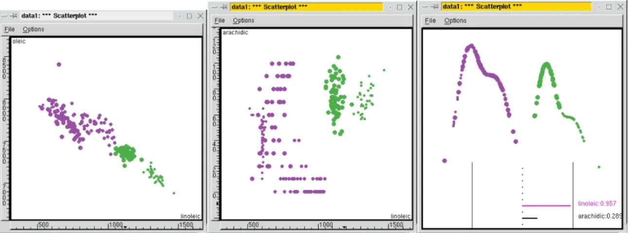
Starting from the three variables found from bivariate plots to be important for separating northern Italian and Sardinian oils we use a higher-dimensional technique to explore them. Using either Rotation, Tour1D or Tour2D examine the separation between the two regions in the 3-dimensional space. Figure 2 shows the results of using Tour1D on the three variables. The two regions can be separated cleanly by a linear combination of linoleic and arachidic acid, roughly corresponding to 0.957×linoleic + 0.289×arachidic.
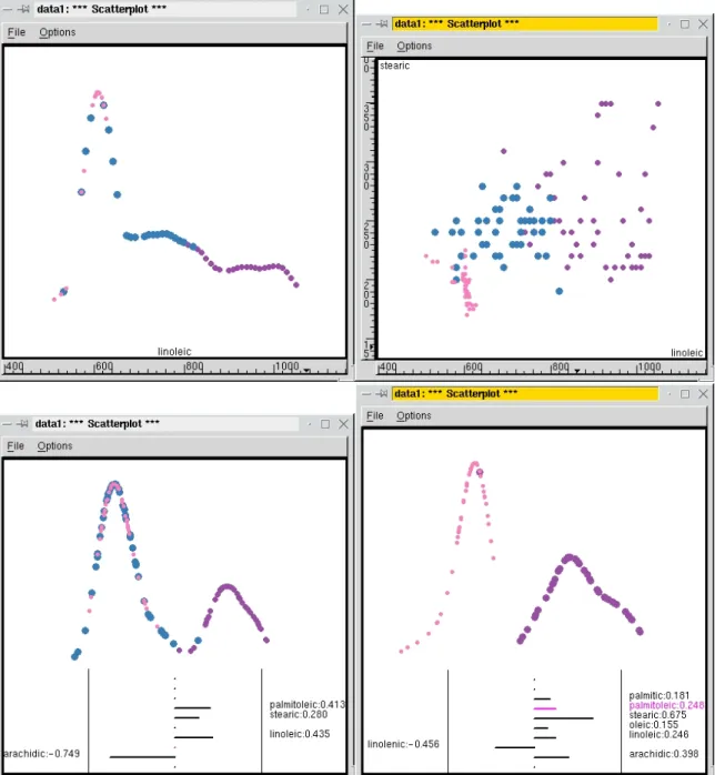
3.2.4 Areas - Northern Italy
There are three areas in the region, Umbria, East and West Liguria. From univariate plots there are no clear separations between areas, although several variables, for example, linoleic acid (Figure 3, show some differences. In bivariate plots, two variables, stearic and linoleic show some differences between the areas. Examining combinations of variables in Tour1D shows that West Liguria is almost separable from the other two areas using palmitoleic, stearic, linoleic and arachidic acids. Umbria and East Liguria are separable, except for one sample, in a combination of most of the variables. To get this result, the projection pursuit controls were used followed by manual manipulation to assess the importance of each variable in the separation of the areas.
Figure 2: Separation between the northern Italian and Sardinian oils in bivariate plots and multivariate plots.
3.2.5 Areas - Sardinia
Separating the oils from the coastal and inland areas of Sardinia can be simply done by using two variables, oleic and linoleic acid.
3.2.6 Areas - Southern Italy
There are four areas in the south Italy region, North and South Apulia, Calabria, Sicily. From univariate plots and bivariate plots there are no clear separations between all four areas. Simplify the work by working with fewer groups, take two of the areas at a time, or three at a time, and plot the data in univariate and bivariate plots. The best results are obtained by removing Sicily. If the oils from this area are removed then the remaining 3 areas are almost separable using the variables palmitic, palmitoleic, stearic and oleic acids. Figure 4 shows plots taken from the Tour2D of these 4 variables revealing the separations between the areas, North and South Apulia, and Calabria. However, the fatty acid content of oils from Sicily is confounded with those of the other areas.
3.2.7 Taking stock
What we have learned from this data is that the olive oils from different geographic regions have dramatically different fatty acid content. The three larger geographic regions, North, South, Sardinia, are well-separated based on eicosenoic, linoleic and arachidic acids. The oils from areas in northern Italy are mostly separable from each other using all the variables. The oils from the inland and coastal areas of Sardinia have different amounts of oleic and linoleic acids. The oils from three of the areas in southern Italy are almost separable. And one is left with the curious content of the oils from Sicily. Why are these oils indistinguishable from the oils of all the other areas in the south? Is there a problem with the quality of these samples?
Figure 4: The areas of southern Italy are mostly separable, except for Sicily.
3.3
Numerical Analysis
The data is broken into training and test samples for this part of the analysis. Approximately 25% of cases within each group are reserved for the test samples. These are the cases used for the test sample, where the data has been sorted by region and area:
1 7 12 15 16 22 27 32 34 35 36 41 50 54 61 68 70 75 76 80 95 101 102 105 106 110 116 118 119 122 134 137 140 147 148 150 151 156 165 175 177 182 183 185 186 187 190 192 194 201 202 211 213 217 218 219 225 227 241 242 246 257 259 263 266 274 280 284 289 291 292 297 305 310 313 314 323 330 333 338 341 342 347 351 352 356 358 359 369 374 375 376 386 392 405 406 415 416 418 420 421 423 426 428 435 440 451 458 460 462 466 468 470 474 476 480 481 482 487 492 493 500 501 509 519 522 530 532 541 543 545 546 551 559 567 570
Region Area # Train # Test South N. Apul. 19 6 South Calabria 42 14 South S. Apul 158 48 South Sicily 27 9 Sard Inland 49 16 Sard Coast 25 8 North E. Lig. 38 12 North W. Lig. 38 12 North Umbria 40 11
We will use what we learned from the visual analysis to guide the numerical analysis. Some methods restrict classification to just two groups, so we will use this restriction with all the classification methods. We will also drop the Sicilian oils from the study - because there is some question raised about the validity of these oils. Here is the binary classification steps we will follow:
3.3.1 Methods Used
Classification trees generate a classification tree by sequentially doing binary splits on variables. Splits are decided on according to the variable and split value which produces the lower measure of impurity. There are several common measures of impurity, Gini and deviance. For example, for a two class problem with 400 observations in each class, denoted as (400,400), variable 1 produces a split of (300,100) and (100,300), and variable 2 produces a split (200,400) and (200,0). The split on variable 2 will produce a lower impurity value because one branch is more pure. There are numerous implementations: R packages such as rpart
and standalone packages such asC4.5, C5.0.
Classical Linear discriminant analysis (LDA) assumes that the populations come from multivariate normal distributions with different mean but equal variance-covariance matrices. Linear boundaries result, and it is possible to reduce the dimension of the data into the space of maximum separation using canonical coordinates. TheMASSpackage in R has functions for LDA.
Quadratic discriminant analysis (QDA) assumes that the populations come from multivariate normal distributions with different mean and different variance-covariance. Non-linear boundaries are the result. TheMASSpackage in R has functions for LDA.
Feed-forward neural networks provide a flexible way to generalize linear regression functions. A simple network model as produced bynnetcode in R (Venables & Ripley 1994) may be represented by the equation:
y=φ(α+ s X h=1 whφ(αh+ p X i=1 wihxi))
the number of nodes in the single hidden layer andφis a fixed function, usually a linear or logistic function. This model has a single hidden layer, and univariate output values.
SVM have recently gained widespread attention due to their success at prediction in classification prob-lems. The subject started in the late seventies (Vapnik 1979). The definitive reference is Vapnik (1999), and Burges (1998) gives a simpler tutorial into the subject. The main difference between this and the previously described classification techniques is that SVMs really only work for separating between 2 groups. There are some modifications for multiple groups but these are little more than one might do manually by working pairwise through the groups. SVM algorithms work by finding a subset of points in the two groups that can be separated, which are then known as the support vectors. These support vectors can be used to define a separating hyperplane, w.x+b = 0, where w =PNS
i=1αiyixi,NS is the number of support vectors, and
α comes from the constraint PNS
i=1αiyi = 0. Actually we search for the support vectors which gives the
hyperplane which gives the biggest separation between the two classes. Note that it is posssible to incorpo-rate non-linear kernel functions allows for defining non-linear separations, and also that modifications allow SVMs to perform well when the classes are not separable. We use the software SVM Light: binary and documentation athttp://svmlight.joachims.org/
3.3.2 The Classification Separating Regions
In separating the southern oils from the other two regions, and then northern oils from Sardinian oils, here is the classification tree solution:
If eicosenoic acid $>$ 7 then the region is South (1) Else
If linoleic $>$ 1053.5 then the region is Sardinia (2) Else the region is North (3)
There are no missclassifications on the first split but the second split is problematic. It is a perfect separation for this data but there is no gap between the two groups. This is easily seen from the plot of the two variables used, Figure 5. So at this point we will shift to using a different method to build a classification rule for northen oils from Sardinian oils.
Here is the R code:
# South vs others d.olive.train<-d.olive[indx.tr,-c(1,2)] d.olive.test<-d.olive[indx.tst,-c(1,2)] c1<-rep(-1,572) c1[d.olive[,1]!=1]<-1 c1.train<-c1[indx.tr] c1.test<-c1[indx.tst] # North vs Sardinia d.olive.train<-d.olive[indx.tr,] c1.train<-c(rep(-1,572))[indx.tr] c1.train[d.olive.train[,1]==3]<-1 c1.train<-c1.train[d.olive.train[,1]!=1] d.olive.train<-d.olive.train[d.olive.train[,1]!=1,-c(1,2)] d.olive.test<-d.olive[indx.tst,] c1.test<-c(rep(-1,572))[indx.tst]
Figure 5: (Left)Plot illustrating the results of tree classifier. (Right) Second boundary from LDA solution, dashed boundary is the tree solution on the LDA predicted values.
c1.test[d.olive.test[,1]==3]<-1 c1.test<-c1.test[d.olive.test[,1]!=1]
d.olive.test<-d.olive.test[d.olive.test[,1]!=1,-c(1,2)] # Trees
# Load the rpart library
olive.rp<-rpart(c1.train~.,data.frame(d.olive.train),method="class") table(c1.train,predict(olive.rp,type="class"))
table(c1.test,predict(olive.rp,data.frame(d.olive.test),type="class"))
Here is the output from R:
# South vs others n= 436
node), split, n, loss, yval, (yprob) * denotes terminal node
1) root 436 190 -1 (0.5642202 0.4357798) 2) eicosenoic>=7 246 0 -1 (1.0000000 0.0000000) * 3) eicosenoic< 7 190 0 1 (0.0000000 1.0000000) * c1.train -1 1 -1 246 0 1 0 190 c1.test -1 1
-1 77 0 1 0 59 # Sardinia vs North n= 190
node), split, n, loss, yval, (yprob) * denotes terminal node
1) root 190 74 1 (0.3894737 0.6105263) 2) linoleic>=1053.5 74 0 -1 (1.0000000 0.0000000) * 3) linoleic< 1053.5 116 0 1 (0.0000000 1.0000000) * c1.train -1 1 -1 74 0 1 0 116 c1.test -1 1 -1 24 0 1 0 35
LDA results in errors in the training sample (error rate = 1/190 = 0.005) and no errors in the test sample. The predicted values are well-separated (see figure) but the boundary is in the wrong place! (See Figure 5, right plot.)
palm palm’oleic stear oleic lino lino’nic arach eico -0.13 -0.27 0.10 0.91 -0.92 -0.24 -0.64 0.03 Table 1: Correlations between predicted values and the predictors.
The variables oleic, linoleic and arachidic are highly correlated with the predicted values (Table 1). The predicted values show a big gap between the northern oils and the sardinian oils but the boundary is set too close to the sardinian group because LDA assumes equal variances.
olive.lda1<-lda(d.olive.train,c1.train) olive.lda1
table(c1.train,predict(olive.lda1,d.olive.train)$class) table(c1.test,predict(olive.lda1,d.olive.test)$class) # plot the predictions of the current sample
olive.x<-predict(olive.lda1,d.olive.train, dimen=1)$x olive.x2<-predict(olive.lda1,d.olive.test, dimen=1)$x olive.lda.proj<-predict(olive.lda1,d.olive[,-c(1,2)],dimen=1)$x par(pty="s") plot(d.olive[,10],olive.lda.proj,type="n", xlab="eicosenoic",ylab="LDA Discrim 1")
points(d.olive[d.olive[,1]==1,10],olive.lda.proj[d.olive[,1]==1],pch="x",col=2) points(d.olive[d.olive[,1]==2,10],olive.lda.proj[d.olive[,1]==2],pch="s",col=3) points(d.olive[d.olive[,1]==3,10],olive.lda.proj[d.olive[,1]==3],pch=16,col=6) abline(v=7) lines(c(0,7),c(-0.49,-0.49)) text(50,7,"South") text(-2,8,"Sardinia",pos=4) text(-2,-6,"North",pos=4)
# Predicted values are generated by
# x’sigma^(-1)(mean1-mean2)-((mean1+mean2)/2)’sigma^(-1)(mean1-mean2) # So these lines should recreate the predicted values.
xmn<-apply(d.olive.train,2,mean)
x<-as.matrix(d.olive.train-matrix(rep(xmn,190),nrow=190,byrow=T))%*% as.matrix(olive.lda1$scaling)
# compute correlations between variables and the predicted values cor(olive.x,d.olive.train[,1]) cor(olive.x,d.olive.train[,2]) cor(olive.x,d.olive.train[,3]) cor(olive.x,d.olive.train[,4]) cor(olive.x,d.olive.train[,5]) cor(olive.x,d.olive.train[,6]) cor(olive.x,d.olive.train[,7]) cor(olive.x,d.olive.train[,8])
These are the results:
Prior probabilities of groups: -1 1
0.3894737 0.6105263 Group means:
palmitic palmitoleic stearic oleic linoleic linolenic arachidic -1 1111.514 95.82432 224.5811 7270.824 1193.757 27.90541 73.85135 1 1095.578 83.52586 231.3879 7790.284 729.250 21.53448 36.79310
eicosenoic -1 1.972973 1 2.017241
Coefficients of linear discriminants: LD1 palmitic 0.0003340794 palmitoleic 0.0152893597 stearic 0.0142798870 oleic 0.0010155503 linoleic -0.0097371901 linolenic -0.0104774449 arachidic -0.0236128945
eicosenoic -0.1193127354 c1.train -1 1 -1 74 0 1 1 115 c1.test -1 1 -1 24 0 1 0 35
Quadratic discriminant analysis provides a perfect classification but its more difficult to determine the location of the boundary between the two groups.
# Quadratic discriminant analysis olive.qda1<-qda(d.olive.train,c1.train) olive.qda1
table(c1.train,predict(olive.qda1,d.olive.train)$class) table(c1.test,predict(olive.qda1,d.olive.test)$class)
Trees calculated on the predicted values provide a perfect classification, although the boundary seems a little too close to the northern oils (Figure 5).
# Check if trees will give a better boundary rpart(c1.train~olive.x,method="class") par(lty=2)
lines(c(0,7),c(-1.49,-1.49)) par(lty=1)
This gives the classification of the regions as: If eicosenoic acid>7 then the region is South (1) Else
If 0.0003×palmitic +0.0153×palmitoleic +0.01423×stearic +0.0010×oleic−0.0097×linoleic
-0.0105×linolenic−0.0236×arachidic−0.1193×eicosenoic - 2.12>-1.49 then the region is Sardinia (2) Else the region is North (3)
There is no error associated with this rule.
Sardinian Oils
Split the samples into training and test sets.
# Sardinian oils d.olive.train<-d.olive[indx.tr,] c1.train<-c(rep(-1,572))[indx.tr] c1.train[d.olive.train[,2]==6]<-1 c1.train<-c1.train[d.olive.train[,1]==2] d.olive.train<-d.olive.train[d.olive.train[,1]==2,-c(1,2)] d.olive.test<-d.olive[indx.tst,] c1.test<-c(rep(-1,572))[indx.tst]
c1.test[d.olive.test[,2]==6]<-1 c1.test<-c1.test[d.olive.test[,1]==2]
d.olive.test<-d.olive.test[d.olive.test[,1]==2,-c(1,2)]
Figure 6: Separation of the inland and coastal Sardinian oils using trees (horizontal axis) and LDA (vertical axis).
A classification tree produces a perfect classification of both training and test samples but the separation between groups is rather small relative to the split for a slightly more complex solution provided by LDA (Figure 6). Here is the code:
# Trees
olive.rp<-rpart(c1.train~.,data.frame(d.olive.train),method="class") olive.rp
table(c1.train,predict(olive.rp,type="class"))
table(c1.test,predict(olive.rp,data.frame(d.olive.test),type="class")) # Linear discriminant analysis
olive.lda1<-lda(d.olive.train,c1.train) olive.lda1
table(c1.train,predict(olive.lda1,d.olive.train)$class) table(c1.test,predict(olive.lda1,d.olive.test)$class) # plot the predictions of the current sample
olive.x<-predict(olive.lda1,d.olive.train, dimen=1)$x olive.x2<-predict(olive.lda1,d.olive.test, dimen=1)$x par(mfrow=c(1,1),pty="s")
plot(c(d.olive.train[,5],d.olive.test[,5]),c(olive.x,olive.x2),type="n", xlab="Tree",ylab="LDA Discrim") points(c(d.olive.train[c1.train==-1,5],d.olive.test[c1.test==-1,5]), c(olive.x[c1.train==-1],olive.x2[c1.test==-1]),pch=16,col=2) points(c(d.olive.train[c1.train==1,5],d.olive.test[c1.test==1,5]), c(olive.x[c1.train==1],olive.x2[c1.test==1]),pch="x",col=4) abline(v=1246.5) abline(h=0.73) text(1150,-4,"Inland",pos=4) text(1260,7,"Coastal",pos=4)
The solution for Sardinian oils then is:
If 0.0097×palmitic +0.0018×palmitoleic +0.0276×stearic +0.00075×oleic +0.0271×linoleic +0.0750×linolenic −0.0260×arachidic−0.0400×eicosenoic - 55.04>0.73 then the sample is from inland Sardinia.
palm palm’oleic stear oleic lino lino’nic arach eico 0.52 0.28 0.73 -0.96 0.98 -0.47 -0.17 -0.01 Table 2: Correlations between variables and predicted values for Sardinian oils.
Based on correlations with the predicted values (Table 2) the important variables for separating inland and coastal Sardinia are oleic, linoleic and stearic acids, with palmitic and linolenic being somewhat important.
Northern Oils
Separating these northern oils is more difficult, based on our visual analysis.
East Liguria vs West Liguria,Umbria
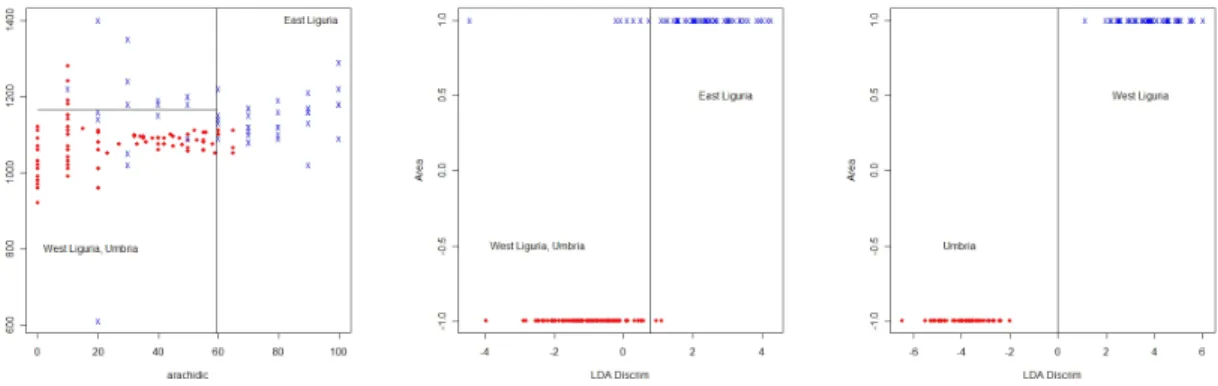
The classification difficulty is reflected in the results of tree classifiers: the error in the training set is 8/116 = 0.07 and the error in the test set is 8/35 = 0.23. But is is a simple solution using just two variables, palmitic and arachidic. (See Figure 7 left plot.)
The LDA solution is a littler better, with 6/116 = 0.05 errors in the training set and 3/35 = 0.09 in the test set (Figure 7).
# East Liguria vs others # Trees olive.rp<-rpart(c1.train~.,data.frame(d.olive.train),method="class") olive.rp table(c1.train,predict(olive.rp,type="class")) table(c1.test,predict(olive.rp,data.frame(d.olive.test),type="class")) plot(c(d.olive.train[,7],d.olive.test[,7]), c(d.olive.train[,1],d.olive.test[,1]),type="n", xlab="arachidic",ylab="palmitic") points(c(d.olive.train[c1.train==-1,7],d.olive.test[c1.test==-1,7]), c(d.olive.train[c1.train==-1,1],d.olive.test[c1.test==-1,1]),pch=16,col=2) points(c(d.olive.train[c1.train==1,7],d.olive.test[c1.test==1,7]), c(d.olive.train[c1.train==1,1],d.olive.test[c1.test==1,1]),pch="x",col=4)
abline(v=59.5)
lines(c(0,59.5),c(1165,1165)) text(80,1400,"East Liguria",pos=4) text(0,800,"West Liguria, Umbria",pos=4) # Linear discriminant analysis
olive.lda1<-lda(d.olive.train,c1.train) olive.lda1 table(c1.train,predict(olive.lda1,d.olive.train)$class) table(c1.test,predict(olive.lda1,d.olive.test)$class) olive.x<-predict(olive.lda1,d.olive.train)$x olive.x2<-predict(olive.lda1,d.olive.test)$x xmn<-apply(d.olive.train,2,mean) x<-as.matrix(d.olive.train-matrix(rep(xmn,79),nrow=79,byrow=T))%*% as.matrix(olive.lda1$scaling) xmn%*%as.matrix(olive.lda1$scaling) plot(c(olive.x,olive.x2),c(c1.train,c1.test),type="n", xlab="LDA Discrim",ylab="Area") points(c(olive.x[c1.train==-1],olive.x2[c1.test==-1]), c(c1.train[c1.train==-1],c1.test[c1.test==-1]),pch=16,col=2) points(c(olive.x[c1.train==1],olive.x2[c1.test==1]), c(c1.train[c1.train==1],c1.test[c1.test==1]),pch="x",col=4) abline(v=0.76) text(2,0.5,"East Liguria",pos=4)
text(-4,-0.5,"West Liguria, Umbria",pos=4)
# compute correlations between variables and the predicted values cor(olive.x,d.olive.train[,1]) cor(olive.x,d.olive.train[,2]) cor(olive.x,d.olive.train[,3]) cor(olive.x,d.olive.train[,4]) cor(olive.x,d.olive.train[,5]) cor(olive.x,d.olive.train[,6]) cor(olive.x,d.olive.train[,7]) cor(olive.x,d.olive.train[,8])
Turning to feed-forward neural networks. After several runs a good result the net converges, to a solution that has no error in the training set but two errors in the test set. The solution is as follows:
Area = 1.01-2.01×(-0.22×palmitic-0.01×palmitoleic-0.13×stearic +0.05×oleic -0.21×linoleic +0.61×linolenic-0.05×arachidic +0.03×eicosenoic) -0.01×(0.07×palmitic+0.03×palmitoleic+0.06× stearic -0.02×oleic +0.05×linoleic -0.05×linolenic+0.04×arachidic) -2.00×(-0.10×palmitic+0.10× palmitoleic+0.11×stearic +0.07×oleic -0.01×linoleic +0.20×linolenic-0.26×arachidic -0.01× eicosenoic)
Figure 7: (Left) Tree solution for East Liguria vs West Liguria,Umbria, (Middle) LDA solution for East Liguria vs West Liguria,Umbria, (Right) LDA solution for West Liguria vs Umbria.
olive.nn<-nnet(c1.train~.,d.olive.train,size=3,linout=T,decay=5e-4, range=0.6,maxit=1000) # weights: 31 initial value 101.133439 iter 10 value 100.792293 iter 20 value 88.353498 ... iter 560 value 0.004900 final value 0.004900 converged > table(c1.train,round(predict(olive.nn,d.olive.train))) c1.train -1 1 -1 79 0 1 0 37 > table(c1.test,round(predict(olive.nn,d.olive.test))) c1.test -3 -1 0 1 -1 0 21 1 0 1 1 0 0 12
Support vector machines (SVM) produce 2 errors in the training set and 6 errors in the test set. The Windows version of SVM light is used. To run SVM the data needs to be outputted to file in a special format. The svm learn and svm classify executables are run in a command window. The parameters needs to be adjusted some to get the best results. Linear kernels are used.
The neural network solution is the best but not substantially different from the LDA solution in test set error. So we will use the LDA solution which is a little simpler.
West Liguria vs Umbria
Trees result in no errors in the training set and 2/22 = 0.09 errors in the test set. LDA results in no errors in either training or test sets (Figure 7).
# West Liguria vs Umbria d.olive.train2<-d.olive[indx.tr,] c2.train<-c(rep(-1,572))[indx.tr] c2.train[d.olive.train2[,2]==8]<-1 c2.train<-c2.train[d.olive.train2[,1]==3&d.olive.train2[,2]!=7] d.olive.train2<-d.olive.train2[d.olive.train2[,1]==3&d.olive.train2[,2]!=7, -c(1,2)] d.olive.test2<-d.olive[indx.tst,] c2.test<-c(rep(-1,572))[indx.tst] c2.test[d.olive.test2[,2]==8]<-1 c2.test<-c2.test[d.olive.test2[,1]==3&d.olive.test2[,2]!=7] d.olive.test2<-d.olive.test2[d.olive.test2[,1]==3&d.olive.test2[,2]!=7,-c(1,2)]
The solution for northern oils then is:
If 0.0285×palmitic +0.0009×palmitoleic +0.0317×stearic +0.0187×oleic +
0.0180×linoleic−0.0264×linolenic +0.0768×arachidic +0.0795×eicosenoic - 200.0>0.76 then the sample is from East Liguria
Else
if 0.0124×palmitic +0.0343×palmitoleic +0.0261×stearic +0.0122×oleic +
0.0172×linoleic−0.0627×linolenic−0.0342×arachidic−0.2244×eicosenoic - 128.0>-0.03 then the sample is from West Liguria
Else it is from Umbria.
palm palm’oleic stear oleic lino lino’nic arach eico E.Lig vs Oth 0.67 0.03 0.21 -0.26 -0.26 0.25 0.76 -0.10 W. Lig vs Umb -0.34 0.80 0.76 -0.88 0.94 -0.93 -0.85 0.05
Table 3: Correlations between variables and predicted values for northern oils.
Based on correlations with the predicted values (Table 3) the important variables for separating East Liguria are palmitic and arachidic, and for separating West Liguria from Umbria the important variables are palmitoleic, stearic, oleic, linoleic, linolenic, arachidic.
Southern Oils
The areas of the southern region promised to be the most difficult to classify. We ignore Sicily to begin. Calabria vs Others
With trees there are 4/219 = 0.018 errors in the training set, and 2/68 = 0.029 errors in the test set. The plots in Figure 8 illustrate the splits. This is about the best solution of all the methods, surprisingly! There are too many errors in the training set, but the most important error to guard against is the test error, and trees give the smallest test error. LDA results in 4/219 = 0.18 errors in the training set and 5/68 = 074 errors in the test set. QDA results in only 1/219 = 0.004 in the training set but 3/68 = 0.044 in the test set. The best results for FFNN were 0 errors in the training set but 3/68−0.044 errors in the test set. SVM had 1 error in the training set and 4 errors in the test set.
Figure 8: The boundaries resulting from a tree classifier on Calabria vs other southern areas.
# Southern oils - without Sicily # Calabria vs Others d.olive.train<-d.olive[indx.tr,] c1.train<-c(rep(-1,572))[indx.tr] c1.train[d.olive.train[,2]==2]<-1 c1.train<-c1.train[d.olive.train[,1]==1&d.olive.train[,2]!=4] d.olive.train<-d.olive.train[d.olive.train[,1]==1&d.olive.train[,2]!=4,-c(1,2)] d.olive.test<-d.olive[indx.tst,] c1.test<-c(rep(-1,572))[indx.tst] c1.test[d.olive.test[,2]==2]<-1 c1.test<-c1.test[d.olive.test[,1]==1&d.olive.test[,2]!=4] d.olive.test<-d.olive.test[d.olive.test[,1]==1&d.olive.test[,2]!=4,-c(1,2)] # Calabria vs Others # Trees olive.rp<-rpart(c1.train~.,data.frame(d.olive.train),method="class") table(c1.train,predict(olive.rp,type="class")) table(c1.test,predict(olive.rp,data.frame(d.olive.test),type="class")) par(pty="s",mfrow=c(1,2)) plot(c(d.olive.train[,1],d.olive.test[,1]), c(d.olive.train[,5],d.olive.test[,5]), type="n",xlab="palmitic",ylab="linoleic",main="First split") points(c(d.olive.train[c1.train==-1,1],d.olive.test[c1.test==-1,1]),
c(d.olive.train[c1.train==-1,5],d.olive.test[c1.test==-1,5]),pch=16,col=2) points(c(d.olive.train[c1.train==1,1],d.olive.test[c1.test==1,1]), c(d.olive.train[c1.train==1,5],d.olive.test[c1.test==1,5]),pch="x",col=4) abline(h=946) text(1000,1400,"Others",pos=4) plot(c(d.olive.train[d.olive.train[,5]<946,1], d.olive.test[d.olive.test[,5]<946,1]), c(d.olive.train[d.olive.train[,5]<946,6], d.olive.test[d.olive.test[,5]<946,6]),
type="n",xlab="palmitic",ylab="linolenic",main="Next two splits") points(c(d.olive.train[c1.train==-1&d.olive.train[,5]<946,1], d.olive.test[c1.test==-1&d.olive.test[,5]<946,1]), c(d.olive.train[c1.train==-1&d.olive.train[,5]<946,6], d.olive.test[c1.test==-1&d.olive.test[,5]<946,6]),pch=16,col=2) points(c(d.olive.train[c1.train==1&d.olive.train[,5]<946,1], d.olive.test[c1.test==1&d.olive.test[,5]<946,1]), c(d.olive.train[c1.train==1&d.olive.train[,5]<946,6], d.olive.test[c1.test==1&d.olive.test[,5]<946,6]),pch="x",col=4) abline(v=1116) lines(c(1116,1500),c(37,37)) text(900,70,"Others",pos=4) text(1300,65,"Calabria",pos=4) # Linear discriminant analysis
olive.lda1<-lda(d.olive.train,c1.train) olive.lda1 table(c1.train,predict(olive.lda1,d.olive.train)$class) table(c1.test,predict(olive.lda1,d.olive.test)$class) olive.x<-predict(olive.lda1,d.olive.train)$x olive.x2<-predict(olive.lda1,d.olive.test)$x # Quadratic discriminant analysis
olive.qda1<-qda(d.olive.train,c1.train) olive.qda1
table(c1.train,predict(olive.qda1,d.olive.train)$class) table(c1.test,predict(olive.qda1,d.olive.test)$class) # FFNN
# Load nnet library
olive.nn<-nnet(c1.train~.,d.olive.train,size=5,linout=T,decay=5e-4, range=0.6,maxit=1000) table(c1.train,round(predict(olive.nn,d.olive.train))) table(c1.test,round(predict(olive.nn,d.olive.test))) olive.x<-predict(olive.nn,d.olive.train) olive.x2<-predict(olive.nn,d.olive.test)
# trees n= 219
node), split, n, loss, yval, (yprob) * denotes terminal node
1) root 219 42 -1 (0.8082192 0.1917808) 2) linoleic>=946 153 0 -1 (1.0000000 0.0000000) * 3) linoleic< 946 66 24 1 (0.3636364 0.6363636) 6) palmitic< 1116 18 0 -1 (1.0000000 0.0000000) * 7) palmitic>=1116 48 6 1 (0.1250000 0.8750000) 14) linolenic< 37 8 3 -1 (0.6250000 0.3750000) * 15) linolenic>=37 40 1 1 (0.0250000 0.9750000) * c1.train -1 1 -1 176 1 1 3 39 c1.test -1 1 -1 54 0 1 2 12 # LDA lda.data.frame(d.olive.train, c1.train) Prior probabilities of groups:
-1 1 0.8082192 0.1917808 Group means:
palmitic palmitoleic stearic oleic linoleic linolenic arachidic -1 1353.311 170.2655 212.2655 7007.458 1121.831 35.54802 61.56497 1 1298.119 120.5952 263.4762 7319.881 808.119 45.54762 64.02381
eicosenoic -1 25.38418 1 28.83333
Coefficients of linear discriminants: LD1 palmitic -0.03604224 palmitoleic -0.05131146 stearic -0.03084686 oleic -0.04136986 linoleic -0.04599853 linolenic 0.06430998 arachidic -0.08761155 eicosenoic -0.09149567
c1.train -1 1 -1 173 4 1 0 42 c1.test -1 1 -1 50 4 1 1 13 # QDA c1.train -1 1 -1 176 1 1 0 42 c1.test -1 1 -1 54 0 1 3 11 # FFNN # weights: 51 initial value 144.303546 iter 10 value 69.334956 ... iter 250 value 0.542601 final value 0.542600 converged c1.train -1 1 -1 177 0 1 0 42 c1.test -1 0 1 -1 53 0 1 1 1 1 12
North vs South Apulia
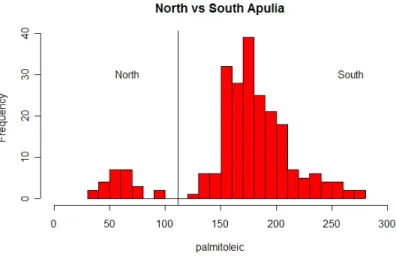
These two areas turn out to be very easy to separate, using trees. The training and test sets are both perfectly classified using palmitoleic acid (Figure 9).
Here is the code:
# North Apulia vs South Apulia d.olive.train2<-d.olive[indx.tr,] c2.train<-c(rep(-1,572))[indx.tr] c2.train[d.olive.train2[,2]==1]<-1 c2.train<-c2.train[d.olive.train2[,1]==1&d.olive.train2[,2]!=2& d.olive.train2[,2]!=4] d.olive.train2<-d.olive.train2[d.olive.train2[,1]==1&d.olive.train2[,2]!=2& d.olive.train2[,2]!=4,-c(1,2)] d.olive.test2<-d.olive[indx.tst,] c2.test<-c(rep(-1,572))[indx.tst]
Figure 9: North and South Apulia can be separated very cleanly using palmitoleic acid. c2.test[d.olive.test2[,2]==1]<-1 c2.test<-c2.test[d.olive.test2[,1]==1&d.olive.test2[,2]!=2& d.olive.test2[,2]!=4] d.olive.test2<-d.olive.test2[d.olive.test2[,1]==1&d.olive.test2[,2]!=2& d.olive.test2[,2]!=4,-c(1,2)] # Trees olive.rp<-rpart(c2.train~.,data.frame(d.olive.train2),method="class") olive.rp table(c2.train,predict(olive.rp,type="class")) table(c2.test,predict(olive.rp,data.frame(d.olive.test2),type="class")) par(mfrow=c(1,1)) hist(c(d.olive.train2[,2],d.olive.test2[,2]),30,col=2,
xlab="palmitoleic",main="North vs South Apulia",xlim=c(0,300)) text(50,30,"North",pos=4)
text(250,30,"South",pos=4) abline(v=111.5)
Here are the results:
n= 177
node), split, n, loss, yval, (yprob) * denotes terminal node
1) root 177 19 -1 (0.8926554 0.1073446)
2) palmitoleic>=111.5 158 0 -1 (1.0000000 0.0000000) * 3) palmitoleic< 111.5 19 0 1 (0.0000000 1.0000000) *
c2.train -1 1 -1 158 0 1 0 19 c2.test -1 1 -1 48 0 1 0 6
Now lets review Sicily
Sicily, the problem area, cannot be cleanly separated from the other areas using trees. The error is 15/246 = 0.061 in the training set, and 7/77 = 0.091 in the test set. What about FFNN or SVM?
Here is the code:
olive.rp<-rpart(c1.train~.,data.frame(d.olive.train),method="class") olive.rp
table(c1.train,predict(olive.rp,type="class"))
table(c1.test,predict(olive.rp,data.frame(d.olive.test),type="class"))
Here are the results:
n= 246
node), split, n, loss, yval, (yprob) * denotes terminal node
1) root 246 27 -1 (0.89024390 0.10975610) 2) eicosenoic< 34.5 199 6 -1 (0.96984925 0.03015075) * 3) eicosenoic>=34.5 47 21 -1 (0.55319149 0.44680851) 6) stearic< 261 30 8 -1 (0.73333333 0.26666667) 12) arachidic< 84.5 23 3 -1 (0.86956522 0.13043478) * 13) arachidic>=84.5 7 2 1 (0.28571429 0.71428571) * 7) stearic>=261 17 4 1 (0.23529412 0.76470588) * c1.train -1 1 -1 213 6 1 9 18 c1.test -1 1 -1 65 3 1 4 5
Thus the solution for the areas of the southern region (without Sicily) is:
If linoleic>=946
If palmitoleic >= 111.5 then the area is South Apulia Else the area is North Apulia
Else (linoleic<946) If palmitic<1116
Else the area is North Apulia Else (palmitic>=1116)
If linolenic<37
If palmitoleic >= 111.5 then the area is South Apulia Else the area is North Apulia
Else (linolenic>37) the area is Calabria
4
Summary
The classification rule (with values given in %×100) is then: Ifeicosenoic acid>7 then the region isSouth
Ifeicosenoic acid<34.5 then the area isSicily Else
Ifstearic<261
Ifarachidic<84.5 the area isSicily
Ifstearic≥261 OR if (stearic<261 and arachidic≥84.5) Iflinoleic≥946
Ifpalmitoleic ≥111.5 the area isSouth Apulia Elsethe area isNorth Apulia
Else(linoleic <946) Ifpalmitic≥1116
Ifpalmitoleic≥111.5 the area isSouth Apulia Elsethe area isNorth Apulia
Else(palmitic≥1116) Iflinolenic<37
Ifpalmitoleic ≥111.5 then the area is South Apulia Elsethe area isNorth Apulia
Else(linolenic>37) the area isCalabria Else
If0.0003×palmitic +0.0153×palmitoleic +0.01423×stearic +0.0010×oleic−0.0097×linoleic
-0.0105×linolenic−0.0236×arachidic−0.1193×eicosenoic - 2.12>-1.49 then the region is Sardinia If0.0097×palmitic +0.0018×palmitoleic +0.0276×stearic +0.00075×oleic +0.0271×linoleic+
0.0750×linolenic−0.0260×arachidic−0.0400×eicosenoic - 55.04>0.73 then the sample is frominland Sardinia
Elsethe sample is fromcoastal Sardinia Elsethe region isNorth
If0.0285×palmitic +0.0009×palmitoleic +0.0317×stearic +0.0187×oleic +
0.0180×linoleic−0.0264×linolenic +0.0768×arachidic +0.0795×eicosenoic - 200.0>0.76 then the sample is fromEast Liguria
Else
if 0.0124×palmitic +0.0343×palmitoleic +0.0261×stearic +0.0122×oleic +
0.0172×linoleic−0.0627×linolenic−0.0342×arachidic−0.2244×eicosenoic - 128.0>-0.03 then the sample is fromWest Liguria
Elseit is from Umbria
The error on the test set overall is (3 + 7 + 2)/136 = 0.09 including Sicily and 5/127 = 0.04 without Sicily, and separately on the areas is given in Table 4. The important variables in each of the separations are given in Table 5.
There are several qualifications about the study:
• We are assuming that the data samples have been collected appropriately, that the samples are repre-sentative of the oils of the areas they are purported to be produced in.
• There is a big difference in the sample sizes for each class. South Apulia is the most abundantly represented and form the internet search of material this is one of the most prolific olive oil producing
Classes Test Error Overall (with Sicily) 12/136=0.09 Overall (without Sicily) 5/127=0.04 South vs Others 0/136 =0 North vs Sardinia 0/59 =0 Inland vs Coastal Sardinia 0/24=0 East Liguria vs Others 3/35=0.09 Umbria vs West Liguria 0/23=0 Sicily vs Others 7/77=0.09 Calabria vs Others 2/68=0.03 North vs South Apulia 0/54=0
Table 4: Prediction errors
Separation palmitic palmitoleic stear oleic linoleic linolenic arachidic eicosenoic Regions South/Others x Sardinia/North x x x Sardinia Coast/Inland x x x North E.Liguria/Others x x W.Liguria/Umbria x x x x x x South Sicily/Others x x x Calab/Others x x x N.Apulia/S.Apulia x
Table 5: This table marks the important variables for each separation.
areas. North Apulia has the least samples, only 25. Perhaps the sample size is indicative of the productivity and should perhaps be incorporated into the classifiers.
References
Burges, C. J. C. (1998), ‘A Tutorial Support Vector Machines for Pattern Recognition’, Data Mining and
Knowledge Discovery2, 121–167.
Forina, M., Armanino, C., Lanteri, S. & Tiscornia, E. (1983), Classification of olive oils from their fatty acid composition,inH. Martens & H. Russwurm Jr., eds, ‘Food Research and Data Analysis’, Applied Science Publishers, London, pp. 189–214.
Vapnik, V. (1979),Estimation of Dependence Based on Empirical Data (In Russian), Nauka, Moscow. Vapnik, V. (1999), The Nature of Statistical Learning Theory (Statistics for Engineering and Information
Science), Springer-Verlag, New York, NY.