Proximal approaches for matrix optimization problems: Application to robust precision matrix estimation

Proximal Approaches for Matrix Optimization Problems: Application to

Robust Precision Matrix Estimation

A. Benfenatia,∗_{, E. Chouzenoux}b_{, J.–C. Pesquet}b

a_{Dipartimento di Scienze e Politiche Ambientali, Universit´a degli studi di Milano, Via Celoria 2, 20133, Milano, Italy} b_{Center for Visual Computing, INRIA Saclay and CentraleSup´elec, University Paris-Saclay, 9 rue Joliot–Curie, 91190,}

Gif–sur–Yvette, France

Abstract

In recent years, there has been a growing interest in mathematical models leading to the minimization, in a symmetric matrix space, of a Bregman divergence coupled with a regularization term. We address problems of this type within a general framework where the regularization term is split into two parts, one being a spectral function while the other is arbitrary. A Douglas–Rachford approach is proposed to address such problems, and a list of proximity operators is provided allowing us to consider various choices for the fit–to–data functional and for the regularization term. Based on our theoretical results, two novel approaches are proposed for the noisy graphical lasso problem, where a covariance or precision matrix has to be statistically estimated in presence of noise. The Douglas–Rachford approach directly applies to the estimation of the covariance matrix. When the precision matrix is sought, we solve a non-convex optimization problem. More precisely, we propose a majorization–minimization approach building a sequence of convex surrogates and solving the inner optimization subproblems via the aforementioned Douglas–Rachford procedure. We establish conditions for the convergence of this iterative scheme. We illustrate the good numerical performance of the proposed approaches with respect to state–of–the–art approaches on synthetic and real-world datasets.

Keywords: Covariance estimation; graphical lasso; matrix optimization; Douglas-Rachford method; majorization-minimization; Bregman divergence

1. Introduction

In recent years, various applications such as shape classification models [1], gene expression [2], model selection [3, 4], computer vision [5], inverse covariance estimation [6, 7, 8, 9, 10, 11, 12], graph estimation

?_{This work was funded by the Agence Nationale de la Recherche under grant ANR-14-CE27-0001 GRAPHSIP and it was} supported by Institut Universitaire de France

∗_{Corresponding author.}

Email addresses: [email protected](A. Benfenati),[email protected](E. Chouzenoux),[email protected](J.–C. Pesquet)

[13, 14, 15, 16], social network and corporate inter-relationships analysis [17], or brain network analysis [18] have led to matrix variational formulations of the form:

minimize

C∈Sn

f(C)−trace (TC) +g(C), (1)

whereSn is the set of real symmetric matrices of dimensionn×n,Tis a givenn×nreal matrix (without

loss of generality, it will be assumed to be symmetric), and f: Sn →]− ∞,+∞] andg:Sn →]− ∞,+∞]

are lower-semicontinuous functions which are proper, in the sense that they are finite at least in one point. It is worth noticing that the notion of Bregman divergence [19] gives a particular insight into Problem (1). Indeed, suppose thatf is a convex function differentiable on the interior of its domain int(domf)6=∅. Let

us recall that, inSn endowed with the Frobenius norm, the f-Bregman divergence betweenC ∈ Sn and Y∈int(domf) is

Df(C,Y) =f(C)−f(Y)−trace (T(C−Y)), (2) whereT=∇f(Y) is the gradient of f atY. Hence, the original problem (1) is equivalently expressed as

minimize

C∈Sn

g(C) +Df(C,Y). (3)

Solving Problem (3) amounts to computing the proximity operator ofgatYwith respect to the divergence

Df _{[20, 21] in the spaceS}

n. In the vector case, such kind of proximity operator has been found to be useful

in a number of recent works regarding, for example, image restoration [22, 23, 24], image reconstruction [25], and compressive sensing problems [26, 27].

In this paper, it will be assumed thatf belongs to the class ofspectral functions [28, Chapter 5, Section 2], i.e., for every permutation matrixΣ∈Rn×n,

(∀C∈ Sn) f(C) =ϕ(Σd), (4)

whereϕ: Rn →]−∞,+∞] is a proper lower semi-continuous convex function anddis a vector of eigenvalues

ofC.

Due to the nature of the problems, in many of the aforementioned applications,gis a regularization function promoting the sparsity ofC. We consider here a more generic class of regularization functions obtained by decomposingg asg0+g1, where g0is a spectral function, i.e., for every permutation matrixΣ∈Rn×n,

(∀C∈ Sn) g0(C) =ψ(Σd), (5)

withψ: _Rn _{→]−∞,+∞] a proper lower semi–continuous function,dstill denoting a vector of the eigenvalues}

ofC, whileg1:Sn→]−∞,+∞] is a proper lower semi–continuous function which cannot be expressed under

a spectral form.

A very popular and useful example encompassed by our framework is the graphical lasso (GLASSO) problem, where f is the minus log-determinant function, g1 is a component–wise `1 norm (of the matrix

elements), andg0≡0. Various algorithms have been proposed to solve Problem (1) in this context, including

the popular GLASSO algorithm [6] and some of its recent variants [29]. We can also mention the dual block coordinate ascent method from [3], the SPICE algorithm [30], the gradient projection method in [1], the Refitted CLIME algorithm [31], various algorithms [8] based on Nesterov’s smooth gradient approach [32], ADMM approaches [33], an inexact Newton method [34], and interior point methods [15, 35]. A related model is addressed in [2, 4], with the additional assumption that the sought solution can be split asC1+C2, where C1is sparse andC2is low–rank. The computation of a sparse+low–rank solution is adressed in [36, 37, 38].

Finally, let us mention the ADMM algorithm from [39], and the incremental proximal gradient approach from [40], both addressing Problem (1) whenf is the squared Frobenius norm,g0is a nuclear norm, andg1

is an element–wise`1 norm.

The main goal of this paper is to propose numerical approaches for solving Problem (1). Two settings will be investigated, namely (i) g1 ≡0, i.e. the whole cost function is a spectral one, (ii)g1 6≡0. In the former case, some general results concerning theDf_{-proximity operator of g0 are provided. In the latter}

case, a Douglas–Rachford (DR) optimization method is proposed, which leads us to calculate the proxim-ity operators of several spectral functions of interest. We then consider applications of our results to the estimation of (possibly low-rank) covariance or precision matrices from noisy observations of multivariate Gaussian random variables. The novelty of our formulation lies in the fact that information on the noise is incorporated into the objective function, while preserving the desirable sparsity properties of the sought matrix. Two variational approaches are proposed for estimating either the covariance matrix or its inverse, depending on the prior assumptions made on the problem. The cost function arising from the first formula-tion is minimized through our proposed DR procedure under mild assumpformula-tions on the involved regularizaformula-tion functions. This procedure represents a valid alternative to other algorithms from the literature (see [40, 39]). In turn, the proposed objective function involved in the second formulation is proved to non–convex. Up to the best of our knowledge, no method is available in the literature to solve this problem. We thus introduce a novel majorization-minimization (MM) algorithm where the inner subproblems are solved by employing the aforementioned DR procedure, and establish convergence guarantees for this method.

The paper is organized as follows. Section 2 briefly discusses the solution of the particular instance of Problem (1) corresponding to g1≡0. Section 3 describes a proximal DR minimization algorithm allowing us to address the problem wheng1 6≡0. Its implementation is discussed for a bunch of useful choices for

the involved functionals. Section 4 presents two matrix minimization problems arising when estimating covariance/precision matrices from noisy realizations of a multivariate Gaussian distribution. While the first one can be solved directly with the DR approach introduced in Section 3, the second non-convex problem is addressed thanks to a novel MM scheme, with inner steps solved with our DR method. In Section 5, a performance comparison of the DR approach for precision matrix estimation with state-of-the-art algorithms is performed. The second part of this section is devoted to numerical experiments that

illustrate the applicability of our MM method and its good performance on synthetic and real–world datasets. Notation: Greek letters usually designate real numbers, bold letters designate vectors in a Euclidean space, capital bold letters indicate matrices. The i–th element of the vectord is denoted bydi. Diag(d) denotes the diagonal matrix whose diagonal elements are the components of d. Dn is the cone of vectors d ∈ Rn whose components are ordered by decreasing values. The symbol vect(C) denotes the vector

resulting from a column–wise ordering of the elements of matrixC. The productA⊗Bdenotes the classical Kronecker product of matricesAandB, whileABdenotes the Hadamard component–wise product. Let Hbe a real Hilbert space endowed with an inner product h·,·i and a normk · k, the domain of a function

f:H →]− ∞,+∞] is domf ={x∈ H |f(x)<+∞}. f is coercive if lim

kxk→+∞f(x) = +∞and supercoercive if lim

kxk→+∞f(x)/kxk= +∞. The Moreau subdifferential off atx∈ H is∂f(x) ={t∈ H |(∀y ∈ H)f(y)≥

f(x) +ht, y−xi}. Γ0(H) denotes the class of lower-semicontinuous convex functions fromHto ]− ∞,+∞]

with a nonempty domain (proper). Iff ∈Γ0(H) is (Gˆateaux) differentiable atx∈ H, then∂f(x) ={∇f(x)}

where ∇f(x) is the gradient of f at x. If a functionf:H →]− ∞,+∞] possesses a unique minimizer on a set E⊂ H, it will be denoted by argmin

x∈E

f(x). If there are possibly several minimizers, their set will be denoted by Argmin

x∈E

f(x). Given a set E, int(E) designates the interior ofE andιE denotes the indicator function of the set, which is equal to 0 over this set and +∞otherwise. In the remainder of the paper, the underlying Hilbert space will beSn, the set of real symmetric matrices equipped with the Frobenius norm,

denoted byk · kF. The matrix spectral norm is denoted by k · kS, the`1 norm of a matrix A= (Ai,j)i,j is kAk1 =Pi,j|Ai,j|. For every p∈[1,+∞[, Rp(A) denotes the Schatten p–norm of A, the nuclear norm

being obtained whenp= 1. Ondenotes the set of orthogonal matrices of dimensionnwith real elements;Sn+

andS++

n denote the set of real symmetric positive semidefinite, and symmetric positive definite matrices,

respectively, of dimension n. Id denotes the identity matrix whose dimension will be understood from

the context. The soft thresholding operator softµ and the hard thresholding operator hardµ of parameter µ∈[0,+∞[ are given by (∀ξ∈R) softµ(ξ) = sign(ξ) max{|ξ| −µ,0}and hardµ(ξ) =ξι{|ξ|>µ}, respectively.

2. Spectral Approach

In this section, we show that, in the particular case wheng1≡0, Problem (1) reduces to the optimization of a function defined onRn. Indeed, the problem then reads:

minimize

C∈Sn

f(C)−trace (TC) +g0(C), (6)

where the spectral forms of f and g0 allow us to take advantage of the eigendecompositions of C and T

in order to simplify the optimization problem, as stated below. Since the results in this section are direct extension of existing ones, the proofs will be skipped. The reader can find more details in the extended version of the paper [41].

Theorem 1. Lett∈_Rn _{be a vector of eigenvalues ofTand letU}

T∈ On be such thatT=UTDiag(t)U>T. Let f and g0 be functions satisfying (4) and (5), respectively, where ϕ and ψ are lower-semicontinuous functions. Assume thatdomϕ∩domψ6=∅and that the function d7→ϕ(d)−d>t+ψ(d)is coercive. Then

a solution to Problem (6)exists, which is given by

b

C=UTDiag(bd)U>T (7)

wheredb is any solution to the following problem:

minimize

d∈Rn

ϕ(d)−d>t+ψ(d). (8)

Before deriving a main consequence of Theorem 1, we need to recall some definitions from convex analysis [42, Chapter 26] [20, Section 3.4]:

Definition 1. Let Hbe a finite dimensional real Hilbert space with normk · kand scalar product h·,·i. Let h:H →]− ∞,+∞]be a proper convex function.

• h is essentially smooth if h is differentiable on int(domh) 6= ∅ and

limn→+∞k∇h(xn)k = +∞ for every sequence (xn)n∈N of int(domh) converging to a point on the

boundary ofdomh.

• h is essentially strictly convex if h is strictly convex on every convex subset of the domain of its subdifferential.

• his a Legendre function if it is both essentially smooth and essentially strictly convex.

• If his differentiable on int(domh)6=_∅, the h-Bregman divergence is the function Dh _{defined on H}2 as (∀(x, y)∈ H2₎ Dh(x, y) =      h(x)−h(y)− h∇h(y), x−yi ify∈int(domf) +∞ otherwise. (9)

• Assume thathis a lower-semicontinuous convex Legendre function and that`is a lower-semicontinuous convex function such that int(domh)∩dom` =6 ∅ and either ` is bounded from below or h+` is

supercoercive. Then, the Dh_{-proximity operator of `is}

proxh<sub>`</sub>: int(domh)→int(domh)∩dom` (10)

y7→argmin

x∈H

In this definition, when h= k · k2_{/2, we recover the classical definition of the proximity operator in [43],}

which is defined overH, for every function`∈Γ0(H), and that will be simply denoted by prox`.

As an offspring of Theorem 1, we then get:

Corollary 1. Letf andg0be functions satisfying (4)and (5), respectively, whereϕ∈Γ0(Rn)is a Legendre

function,ψ∈Γ0(Rn),int(domϕ)∩domψ6=∅, and eitherψis bounded from below orϕ+ψis supercoercive.

Then, the Df-proximity operator of g0 is defined at every Y ∈ Sn such that Y = UYDiag(y)U>Y with

UY∈ On andy∈int(domϕ), and it is expressed as

proxf_g 0(Y) =UYDiag(prox ϕ ψ(y))U > Y. (11)

Remark 1. Corollary 1 extends known results concerning the case when f =

k · kF/2 [44]. A rigorous derivation of the proximity operator of spectral functions inΓ0(Sn) for the stan-dard Frobenius metric can be found in [45, Corollary 24.65]. We recover a similar result by adopting a more general approach. In particular, it is worth noticing that Theorem 1 does not require any convexity assumption.

3. Proximal Iterative Approach

Let us now turn our attention to the more general case of the resolution of Problem (1) whenf ∈Γ0(Sn)

and g1 6≡ 0. Proximal splitting approaches for finding a minimizer of a sum of non-necessarily smooth functions have attracted a large interest in the last years [46, 47, 48, 49]. In these methods, the functions can be dealt with either via their gradient or their proximity operator depending on their differentiability properties. In this section, we first list a number of proximity operators of scaled versions off−trace (T·)+g0, wheref andg0, satisfying (4) and (5), are chosen among several options that can be useful in a wide range of practical scenarios. Based on these results, we then propose a proximal splitting Douglas-Rachford algorithm to solve Problem (1).

3.1. Proximity Operators

By definition, computing the proximity operator ofγ(f−trace (T·) +g0) withγ ∈]0,+∞[ atC ∈ Sn

amounts to find a minimizer of the function

C7→f(C)−trace (TC) +g0(C) +

1

2γkC−Ck 2

F (12)

over Sn. The (possibly empty) set of such minimizers is denoted by

Proxγ(f−trace(T·)+g0)(C). As pointed out in Section 2, if f +g0 ∈ Γ0(Sn) then this set is the singleton {prox_{γ(f−trace(T·)+g0)}(C)}. We have the following characterization of this proximity operator:

Theorem 2. Let γ ∈]0,+∞[ andC ∈ Sn. Letf and g0 be functions satisfying (4) and (5), respectively, whereϕ∈Γ0(Rn)andψis a lower-semicontinuous function such thatdomϕ∩domψ6=∅. Letλ∈Rn and

U∈ On be such thatC+γT=UDiag(λ)U>.

(i) Ifψis lower bounded by an affine function thenProxγ(ϕ+ψ)(λ)6=∅and, for everyλb∈Proxγ(ϕ+ψ)(λ), UDiag(bλ)U>∈Proxγ(f−trace(T·)+g0)(C). (13) (ii) If ψis convex, then

prox_{γ(f−trace(T·)+g0)}(C) =UDiagprox_γ(ϕ+ψ)(λ)U>. (14)

Proof. See Appendix A.

We will next focus on the use of Theorem 2 for three choices forf, namely the classical squared Frobenius norm, the minus log det functional, and the Von Neumann entropy, each choice being coupled with various possible choices forg0.

3.1.1. First Example: Squared Frobenius Norm A suitable choice in Problem (1) isf =k · k2

F/2 [39, 40, 50]. The squared Froebenius norm is the spectral

function associated with the functionϕ= k · k2_{/2. It is worth mentioning that this choice forf allows us}

to rewrite the original Problem (1) under the form (3), where ∀(C,Y)∈ S2 n Df(C,Y) =1 2kC−Yk 2 F. (15)

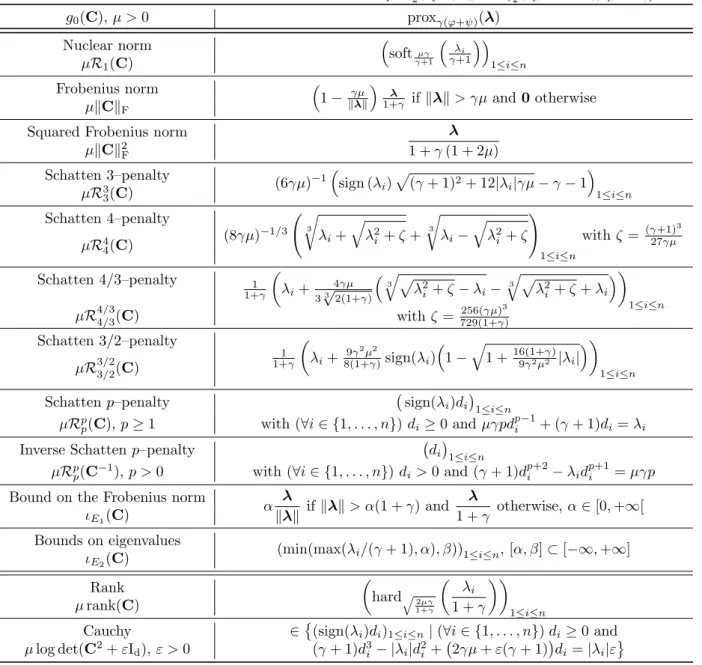
We have thus re-expressed Problem (1) as the determination of a proximal point of function g at T in the Frobenius metric. Table 1 presents several examples of spectral functionsg0 and the expression of the proximity operator ofγ(ϕ+ψ) withγ∈]0,+∞[. These expressions were established by using the properties of proximity operators of functions defined on_Rn _{(see [51, Example 4.4] and [46, Tables 10.1 and 10.2]).} Remark 2. Another option forg0is to choose it equal to µk · kSwhereµ∈]0,+∞[. For every γ∈]0,+∞[, we have then (∀λ∈Rn) proxγ(ϕ+ψ)(λ) = prox₁₊µγ_γk·k+∞ _λ 1 +γ , (16)

wherek · k+∞ is the infinity norm ofRn. By noticing thatk · k+∞is the conjugate function of the indicator function of B`1, the unit `1 ball centered at 0 of _Rn, and using Moreau’s decomposition formula, [45, Proposition 24.8(ix)] yields

(∀λ∈_Rn_{) prox} γ(ϕ+ψ)(λ) = 1 1 +γ λ−µγproj_B `1 _λ µγ . (17)

Table 1: Proximity operators of γ(1 2k · k

2

F+g0) with γ > 0 evaluated at symmetric matrix with vector of eigenvalues

λ= (λi)1≤i≤n. For the inverse Schatten penalty, the function is set to +∞when the argumentCis not positive definite.

E1 denotes the set of matrices inSn with Frobenius norm less than or equal toα and E2 the set of matrices inSn with eigenvalues betweenαandβ. In the last line, thei-th component of the proximity operator is obtained by searching among the nonnegative roots of a third order polynomial those minimizingλ0

i7→ 1 2(λ 0 i− |λi|)2+γ 1₂(λi0)2+µlog((λ0i)2+ε) . g0(C), µ >0 proxγ(ϕ+ψ)(λ) Nuclear norm softµγ γ+1 _λ i γ+1 1≤i≤n µR1(C) Frobenius norm 1− γµ kλk λ 1+γ ifkλk> γµand0otherwise µkCkF

Squared Frobenius norm λ

1 +γ(1 + 2µ)

µkCk2 F

Schatten 3–penalty _(6γµ)−1_{sign (λ} i) p (γ+ 1)2_{+ 12|λ} i|γµ−γ−1 1≤i≤n µR3 3(C) Schatten 4–penalty (8γµ)−1/3 3 r λi+ q λ2 i +ζ+ 3 r λi− q λ2 i +ζ ! 1≤i≤n withζ=(γ+1)_27γµ3 µR4 4(C) Schatten 4/3–penalty ₁ 1+γ λi+ 4γµ 3√3_2(1+γ) 3 q p λ2 i +ζ−λi− 3 q p λ2 i +ζ+λi 1≤i≤n µR4/3_4/3(C) withζ= _729(1+γ)256(γµ)3 Schatten 3/2–penalty 1 1+γ λi+ 9γ 2_µ2 8(1+γ)sign(λi) 1−q1 + 16(1+γ)_9γ2µ2 |λi| 1≤i≤n µR3/2_3/2(C)

Schattenp–penalty sign(λi)di

1≤i≤n µRp

p(C),p≥1 with (∀i∈ {1, . . . , n})di≥0 andµγpd p−1

i + (γ+ 1)di=λi

Inverse Schattenp–penalty di_1≤i≤n

µRp p(C−1),p >0 with (∀i∈ {1, . . . , n})di >0 and (γ+ 1)d p+2 i −λid p+1 i =µγp

Bound on the Frobenius norm

α λ kλk ifkλk> α(1 +γ) and λ 1 +γ otherwise,α∈[0,+∞[ ιE₁(C) Bounds on eigenvalues (min(max(λi/(γ+ 1), α), β))_1≤i≤n, [α, β]⊂[−∞,+∞] ιE2(C) Rank hardq 2µγ 1+γ λi 1 +γ 1≤i≤n µrank(C) Cauchy ∈

(sign(λi)di)1≤i≤n|(∀i∈ {1, . . . , n})di≥0 and µlog det(C2_+εI

d),ε >0 (γ+ 1)d3i − |λi|d2i + 2γµ+ε(γ+ 1)

3.1.2. Second Example: Logdet Function

Another popular choice for f is the negative logarithmic determinant function [1, 33, 2, 13, 3, 6, 15, 4], which is defined as follows

(∀C∈ Sn) f(C) =      −log det(C) ifC∈ S++ n +∞ otherwise. (18)

The above function satisfies property (5) with

∀λ= (λi)1≤i≤n∈Rn ϕ(λ) =        − n X i=1 log(λi) ifλ∈]0,+∞[n +∞ otherwise. (19)

Actually, for a given positive definite matrix, the value of function (18) simply reduces to the Burg entropy of its eigenvalues. Here again, if Y ∈ S++

n and T= −Y−1, we can rewrite Problem (1) under the form

(3), so that it becomes equivalent to the computation of the proximity operator of g with respect to the Bregman divergence given by

(∀C∈ Sn) Df(C,Y) =      logdet(Y) det(C) + trace Y−1C−n ifC∈ S++ n +∞ otherwise. (20)

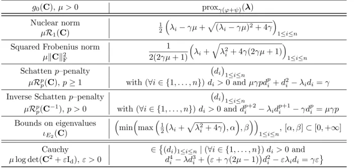
In Table 2, we list some particular choices forg0, and provide the associated closed form expression of the proximity operator proxγ(ϕ+ψ) forγ ∈]0,+∞[, whereϕis defined in (19). These expressions were derived

from [46, Table 10.2].

Remark 3. Letg0be any of the convex spectral functions listed in Table 2. LetWbe an invertible matrix in

Rn×n, and letC∈ SnFrom the above results, one can deduce the minimizer ofC7→γ(f(C)+g0(WCW>))+ 1

2kWCW

>_−Ck2

F whereγ∈]0,+∞[. Indeed, by making a change of variable and by using basic properties of thelog detfunction, this minimizer is equal toW−1_prox

γ(f+g0)(C)(W −1₎>_. 3.1.3. Third Example: Von Neumann Entropy

Our third example is the negative Von Neumann entropy, which appears to be useful in some quantum mechanics problems [54]. It is defined as

(∀C∈ Sn) f(C) =      trace (Clog(C)) ifC∈ S+ n +∞ otherwise. (21)

In the above expression, ifC=UDiag(λ)U> with λ= (λi)1≤i≤n ∈]0,+∞[n and U∈ On, then log(C) = UDiag (logλi)1≤i≤nU>. The logarithm of a symmetric definite positive matrix is uniquely defined and

Table 2: Proximity operators ofγ(f+g0) with γ >0 and f given by (18), evaluated at a symmetric matrix with vector

of eigenvalues λ= (λi)1≤i≤n. For the inverse Schatten penalty, the function is set to +∞when the argumentC is not positive definite. E2 denotes the set of matrices inSnwith eigenvalues betweenαandβ. In the last line, thei-th component of the proximity operator is obtained by searching among the positive roots of a fourth order polynomial those minimizing

λ0_i7→1 2(λ 0 i−λi)2+γ µlog((λ0i)2+ε)−logλ 0 i .

g

(

C

),

µ >

0

prox

(

λ

)

Nuclear norm

λ

−

γµ

+

p

(

λ

−

γµ

)

+ 4

γ

µ

R

(

C

)

Squared Frobenius norm

1

2(2

γµ

+ 1)

λ

+

q

λ

+ 4

γ

(2

γµ

+ 1)

µ

k

C

k

Schatten

p

–penalty

d

µ

R

(

C

),

p

≥

1

with (

∀

i

∈ {

1

, . . . , n

}

)

d

>

0 and

µγpd

+

d

−

λ

d

=

γ

Inverse Schatten

p

–penalty

d

µ

R

(

C

),

p >

0

with (

∀

i

∈ {

1

, . . . , n

}

)

d

>

0 and

d

−

λ

d

−

γd

=

µγp

Bounds on eigenvalues

min

max

λ

+

p

λ

+ 4

γ

, α

, β

, [

α, β

]

⊂

[0

,

+

∞

]

ι

C

)

Cauchy

∈

(

d

)

|

(

∀

i

∈ {

1

, . . . , n

}

)

d

>

0 and

µ

log det(

C

+

ε

I

),

ε >

0

d

−

λd

+

ε

+

γ

(2

µ

−

1)

d

−

ελ

d

=

γε

the functionC7→Clog(C) can be extended by continuity onS+

n similarly to the case whenn= 1. Thus, f is the spectral function associated with

∀λ= (λi)1≤i≤n ∈Rn ϕ(λ) =        n X i=1

λilog(λi) ifλ∈[0,+∞[n

+∞ otherwise.

(22)

Note that the Von Neumann entropy defined for symmetric matrices is simply equal to the well–known Shannon entropy [55] of the input eigenvalues. With this choice for functionf, by settingT= log(Y) + Id

where Y ∈ S++

n , Problem (1) can be recast under the form (3), so that it becomes equivalent to the

computation of the proximity operator ofgwith respect to the Bregman divergence associated with the Von Neumann entropy: (∀C∈ Sn) Df(C,Y) =     

trace (Clog(C)−Ylog(Y)−(log(Y) + Id) (C−Y)) ifC∈ Sn+

+∞ otherwise.

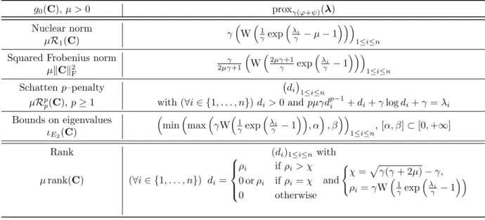
We provide in Table 3 a list of closed form expressions of the proximity operator ofγ(f+g0) for several

Table 3: Proximity operators ofγ(f+g0) with γ >0 and f given by (21), evaluated at a symmetric matrix with vector

of eigenvaluesλ= (λi)1≤i≤n. E2 denotes the set of matrices inSn with eigenvalues betweenα andβ. W(·) denotes the W-Lambert function [56]. g0(C),µ >0 proxγ(ϕ+ψ)(λ) Nuclear norm γ W 1 γexp λi γ −µ−1 1≤i≤n µR1(C)

Squared Frobenius norm γ

2µγ+1 W 2µγ+1 γ exp λi γ −1 1≤i≤n µkCk2 F Schattenp–penalty di 1≤i≤n µRp

p(C),p≥1 with (∀i∈ {1, . . . , n})di>0 andpµγdpi−1+di+γlogdi+γ=λi

Bounds on eigenvalues min max γW 1 γexp λi γ −1 , α , β 1≤i≤n, [α, β]⊂[0,+∞] ιE2(C) Rank (di)1≤i≤n with µrank(C) (∀i∈ {1, . . . , n}) di=      ρi ifρi> χ 0 orρi ifρi=χ 0 otherwise and ( χ=pγ(γ+ 2µ)−γ, ρi=γW 1 γexp λi γ −1 3.2. Douglas-Rachford Algorithm

We now propose a Douglas-Rachford (DR) approach ([57, 46, 58]) for numerically solving Problem (1). We point out that the DR algorithm is directly related to the Alternating Direction Method of Multipliers (ADMM), since the latter can be viewed as a version of the former applied to a dual formulation of the problem. The DR method minimizes the sum of f −trace (T·) +g0 and g1 by alternately computing proximity operators of each of these functions. Proposition 2 allows us to calculate the proximity operator of γ(f −trace (T·) +g0) with γ ∈]0,+∞[, by possibly using the expressions listed in Tables 1, 2, and 3. Sinceg1is not a spectral function, proxγg1 has to be derived from other expressions of proximity operators. For instance, ifg1 is a separable sum of functions of its elements, e.g. g =k · k1, standard expressions for

the proximity operator of vector functions can be employed [51, 46].1

The computations to be performed are summarized in Algorithm 1. We state a convergence theorem in the matrix framework, which is an offspring of existing results in arbitrary Hilbert spaces (see, for example, [46] and [59, Proposition 3.5]).

Theorem 3. Let f and g0 be functions satisfying (4) and (5), respectively, where ϕ ∈ Γ0(Rn) and ψ ∈

Γ0(Rn). Let g1 ∈Γ0(Sn) be such that f−trace (T·) +g0+g1 is coercive. Assume that the intersection of the relative interiors of the domains of f+g0 and g1 is non empty. Let (α(k)₎

k≥0 be a sequence in[0,2] such thatP+∞

k=0α

(k)_(2−α(k)_{) = +∞. Then, the sequences(C}(k+1

2))_k≥0and prox

γg1(2C

(k+1

2)−C(k))

k≥0 generated by Algorithm 1 converge to a solution to Problem (1) whereg=g0+g1.

Algorithm 1Douglas–Rachford Algorithm for solving Problem (1)

1: LetTbe a given matrix inSn, setγ >0 andC(0)∈ Sn.

2: fork= 0,1, . . . do

3: DiagonalizeC(k)_{+γT, i.e. findU}(k)_{∈ O}

n andλ(k)∈Rn such that

C(k)+γT=U(k)Diag(λ(k))(U(k))> 4: d(k+1 2)∈Prox_γ(ϕ+ψ) λ(k) 5: C(k+1 2)=U(k)Diag(d(k+12))(U(k))> 6: Chooseα(k)∈[0,2] 7: C(k+1)_∈C(k)_+α(k)_Prox γg1(2C (k+1 2)−C(k))−C(k+ 1 2) . 8: end for

We have restricted the above convergence analysis to the convex case. Note however that recent convergence results for the DR algorithm in a non-convex setting are available in [60, 61] for specific choices of the involved functionals.

3.3. Positive Semi-Definite Constraint

Instead of solving Problem (1), one may be interested in: minimize

C∈S+ n

f(C)−trace (CT) +g(C), (23)

when domf∩domg6⊂ S+

n. This problem can be recast as minimizing overSnf−trace (·T) +_eg0+g1where

e

g0=g0+ι_S+

n. We are thus coming back to the original formulation whereg0e has been substituted forg0. In order to solve this problem with the proposed proximal approach, a useful result is stated below.

Theorem 4. Let γ ∈]0,+∞[ andC ∈ Sn. Letf and g0 be functions satisfying (4) and (5), respectively, whereϕ∈Γ0(Rn)andψ∈Γ0(Rn). Assume that

∀λ0 = (λ0_i)1≤i≤n ∈Rn ϕ(λ0) +ψ(λ0) =

n

X

i=1

ρi(λ0i) (24)

where, for everyi∈ {1, . . . , n},ρi:R→]−∞,+∞]is such thatdomρi∩[0,+∞[6=∅. Letλ= (λi)1≤i≤n∈Rn

andU∈ On be such thatC+γT=UDiag(λ)U>. Then

prox_{γ(f−trace(T·)+}

e

g0)(C) =UDiag

max(0,prox_γρi(λi))

1≤i≤n

U>. (25)

Proof. Expression (25) readily follows from Theorem 2(ii) and [62, Proposition 2.2].

4. Robust Estimation in Gaussian Graphical Models

Estimating the covariance matrix of a random vector is a key problem in statistics, signal processing, and machine learning [17, 18, 8, 6, 63]. A related problem can be found in graphical modeling: in this case,

the problem consists of estimating the graph adjacency matrix, which is modeled as the precision matrix (i.e., the inverse of covariance matrix) of the random Gaussian vector associated with the nodes of the graph. Nonetheless, in existing techniques devoted to solve the aforementioned problems, little attention is usually paid to the presence of noise corrupting the available observations. We develop in this section two novel formulations which account for noise information. Firstly, we address the problem of covariance matrix estimation. The chosen objective function consists of a squared Frobenius norm term coupled with regularization functions driven by the targeted application, and it can be minimized efficiently by using our DR method. The second problem is the estimation of the precision matrix under sparsity constraints. To the best of our knowledge, no method is available in the literature to solve the non-convex problem arising in this case. Here, we propose to resort to a majorization-minimization (MM) strategy, combined with the previously described DR procedure. Note that a different MM formulation for estimating sparse covariance matrices was proposed in the seminal work in [9].

4.1. Models and Proposed Approaches

LetS∈ S+

n be a sample estimate of a covariance matrixΣwhich is assumed to be decomposed as

Σ=Y∗+σ2Id (26)

whereσ∈[0,+∞[ and Y∗∈ S+

n may have a low-rank structure. We focus on the problem of searching an

estimate ofY∗_{fromSby assuming thatσis known. More specifically, we consider the following observation} model [64]:

(∀i∈ {1, . . . , N}) x(i)=As(i)+e(i) (27) where A∈ Rn×m with m≤ n and, for everyi ∈ {1, . . . , N}, s(i) ∈Rm and e(i) ∈ Rn are realizations of

mutually independent identically distributed Gaussian multivalued random variables with zero mean and covariance matricesP∈ S++

m and σ2Id, respectively. The latter model has been employed for instance in

[65, 66] in the context of the “Relevant Vector Machine problem”. The covariance matrix Σ of the noisy input data x(i)

1≤i≤N takes the form (26) with Y

∗ _=APA>_{. A rough estimate of Σ from the observed} data x(i)

1≤i≤N can be obtained through the empirical covariance: S= 1 N N X i=1 x(i) x(i)>. (28)

In the following, we propose two alternative variational approaches for the estimation ofΣgiven the noisy input data x(i)

1≤i≤N.

Covariance-based model. Our first formulation yields an estimateYb ofY∗ given by

b Y= argmin Y∈S+ n 1 2kY− S+σ 2_I dk2F+g0(Y) +g1(Y), (29)

whereSis the empirical covariance matrix,g0satisfies (5) withψ∈Γ0(Rn),g1∈Γ0(Sn), and the intersection

of the relative interiors of the domains ofg0 andg1 is assumed to be non empty.

A particular instance of this model withσ= 0, g0 =µ0R1,g1=µ1k · k1, and (µ0, µ1)∈[0,+∞[2 was

investigated in [39] and [40] for estimating sparse low-rank covariance matrices. In the latter reference, an application to real data processing arising from protein interaction and social network analysis was presented. One can observe that Problem (29) takes the form (23) by settingf = 1₂k · k2

FandT=S−σ 2_I

d. This allows

us to solve (29) with Algorithm 1. Sinceg0 is assumed to satisfy (5), the proximity step on f+g0+ι_S+ n can be performed by employing Theorem 4 and formulas from Table 1. The resulting DR procedure can thus be viewed as an alternative to the methods developed in [40] and [39]. Let us emphasize that these two algorithms were devised to solve an instance of (29) corresponding to the aforementioned specific choices for g0 and g1, while our approach leaves more freedom in the choice of the regularization functions. A

comparison of the three algorithms will be performed in Section 5.

Precision-based model. Our second strategy focuses on the estimation of the inverse of the covariance matrix, i.e. theprecision matrixC∗= (Y∗)−1 _{by assuming thatY}∗_{∈ S}++

n but may have very small eigenvalues in

order to model a possible low-rank structure. Tackling the problem from this viewpoint leads us to propose the following penalized negative log-likelihood cost function:

(∀C∈ Sn) F(C) =f(C) +TS(C) +g0(C) +g1(C) (30) where (∀C∈ Sn) f(C) =      log det C−1_+σ2_I d ifC∈ S++ n +∞ otherwise, (31) (∀C∈ Sn) TS(C) =      trace Id+σ2C −1 CS ifC∈ S+ n +∞ otherwise, (32)

g0∈Γ0(Sn) satisfies (5) withψ∈Γ0(Rn), andg1∈Γ0(Sn). Typical choices of interest for the latter two

functions are (∀C∈ Sn) g0(C) =      µ0R1(C−1) ifC∈ Sn++ +∞ otherwise, (33)

andg1=µ1k · k1with (µ0, µ1)∈[0,+∞[2. The first function serves to promote a desired low-rank property

by penalizing small eigenvalues of the precision matrix, whereas the second one enforces the sparsity of this matrix as it is usual in graph inference problems. Note that the standard graphical lasso framework [6] is then recovered by settingσ = 0 and µ0 = 0. The advantage of our formulation is that it allows us to consider more flexible variational models while accounting for the presence of noise corrupting the observed

data. The main difficulty however is that Algorithm 1 (or its dual counterpart ADMM) cannot be directly applied to minimize the non-convex costF. In Section 4.2, we study in more details the properties of the latter cost function. This leads us to derive a novel optimization algorithm based on the MM principle, making use of our previously developed Douglas-Rachford scheme for its inner steps.

4.2. Study of Objective FunctionF

The following lemma will reveal useful in our subsequent analysis.

Lemma 1. Letσ∈]0,+∞[. Leth: ]0, σ−2_[→

Rbe a twice differentiable function and let

u: [0,+∞[→R:λ7→ λ

1 +σ2_λ. (34)

The compositionh◦uis convex on ]0,+∞[ if and only if

(∀υ∈]0, σ−2[) ¨h(υ)(1−σ2υ)−2σ2h˙(υ)≥0, (35) whereh˙ (resp. ¨h) denotes the first (resp. second) derivative of h.

Proof. The result directly follows from the calculation of the second-order derivative ofh◦u.

Let us now note thatf is a spectral function fulfilling (4) with

∀λ= (λi)1≤i≤n∈Rn ϕ(λ) =        − n X i=1 log u(λi) ifλ∈]0,+∞[n +∞ otherwise, (36)

where uis defined by (34). According to Lemma 1 (withh=−log), f ∈Γ0(Sn). Thus, the assumptions

made ong0andg1, allow us to deduce thatf +g0+g1 is convex and lower-semicontinuous onSn.

Let us now focus on the properties of the second term in (30).

Lemma 2. LetS∈ S+

n. The function TS in (32)is concave on Sn+.

Proof. See Appendix B.

As a last worth mentioning property, TS is bounded on Sn++. So, if domf ∩domg0∩domg1 6= ∅ and

f+g0+g1is coercive, then there exists a minimizer ofF. Because of the form off, the coercivity condition

is satisfied ifg0+g1 is lower bounded and lim_C∈S+

n,kCk→+∞g0(C) +g1(C) = +∞.

4.3. Minimization Algorithm forF

In order to find a minimizer ofF, we propose aMajorize–Minimize(MM) approach, following the ideas in [67, 64, 68, 69, 70, 71]. At each iteration of an MM algorithm, one constructs a tangent function that majorizes the given cost function and is equal to it at the current iterate. The next iterate is obtained by

minimizing this tangent majorant function, resulting in a sequence of iterates that reduces the cost function value monotonically. According to the results stated in the previous section, our objective function reads as a difference of convex terms. We propose to build a majorizing approximation of functionTSatC0 ∈ Sn++

by exploiting Lemma 2 and the classical concavity inequality onTS:

(∀C∈ Sn++) TS(C)≤ TS(C0) + trace (∇TS(C0) (C−C0)). (37)

Asf is finite only onS++

n , a tangent majorant of the cost function (30) atC0 reads:

(∀C∈ Sn) G(C|C0) =f(C) +TS(C0) + trace (∇TS(C0) (C−C0)) +g0(C) +g1(C).

This leads to the general MM scheme: (∀`∈N) C(`+1)∈Argmin C∈Sn f(C) + trace ∇TS(C(`))C +g0(C) +g1(C) (38) with C(0) ∈ S++

n . At each iteration of the MM algorithm, we have then to solve a convex optimization

problem of the form (1). In the case when g1 ≡ 0, we can employ the procedure described in Section 2 to perform this task in a direct manner. The presence of a regularization termg1 6≡0 usually prevents us to have an explicit solution to the inner minimization problem involved in the MM procedure. We then propose in Algorithm 2 to resort to the Douglas–Rachford approach in Section 3 to solve it iteratively. A convergence result is next stated, which is inspired from [72] (itself relying on [73, p. 6]), but does not require the differentiability ofg0+g1.

Algorithm 2MM algorithm with DR inner steps

1: LetS∈ S+

n be the data matrix. Letϕbe as in (36), letψ∈Γ0(Rn) be associated withg0. Let (γ`)`∈N be a sequence in ]0,+∞[. SetC(0,0)_=C(0)_{∈ S}++

n .

2: for`= 0,1, . . . do 3: fork= 0,1, . . . do

4: ComputeU(`,k)∈ On andλ(`,k)∈Rn such that

C(`,k)−γ`∇TS(C(`)) =U(`,k)Diag(λ(`,k)) U(`,k) > 5: d(`,k+12) = prox γ`(ϕ+ψ) λ (`,k) 6: C(`,k+12) =_U(`,k)<sub>Diag</sub> d(`,k+12) U(`,k)>

7: if Convergence of MM sub-iteration is reachedthen 8: C(`+1)<sub>=C</sub>(`,k+1

2)

9: C(`+1,0)<sub>=C</sub>(`,k)

10: exitinner loop

11: end if 12: Chooseα`,k∈]0,2[ 13: C(`,k+1)=C(`,k)+α`,kproxγ`g1 2C(`,k+12)−_C(`,k) −C(`,k+12) 14: end for 15: end for

Theorem 5. Let (C(`)₎

`≥0 be a sequence generated by (38). Assume that

domf ∩domg0 ∩domg1 6= _∅, f +g0 +g1 is coercive, and E = {C ∈ Sn | F(C) ≤ F(C(0))} is a subset of the relative interior of domg0∩domg1. Then, the following properties hold:

(i) F(C(`))<sub>`≥0</sub> is a decaying sequence converging toF ∈b R. (ii) (C(`)₎

`≥0 has a cluster point.

(iii) Every cluster pointCb of(C(`))`≥0is such thatF(Cb) =Fband it is a critical point ofF, i.e. −∇f(bC)− ∇TS(Cb)∈∂(g0+g1)(bC).

Proof. See Appendix C.

5. Numerical Experiments

This section presents some numerical tests illustrating the validity of the proposed algorithms. All the tests were ran on a Hewlett–Packard Notebook with 16GB or RAM, INTEL i5 CPU (1.6GHz) equipped with MatLab R2019a. All the numerical tests are reproducible, using the code we made available athttp:

//www-syscom.univ-mlv._{fr/~benfenat/Software}.html.

5.1. Application to Sparse Covariance Matrix Estimation

We first consider the application of the DR algorithm from Section 3 to the sparse covariance matrix estimation problem introduced in [40]. As we have shown in Section 4.1, a solution to this problem can be obtained by solving the penalized least-squares problem (29), where S is the empirical covariance matrix defined in (28), and the regularization terms areg0=µ0R1 andg1=µ1k · k1. We propose to compare the

performance of the DR approach from Section 3.2, with the IPD algorithm [40] and the ADMM procedure [39], for solving this convex optimization problem. The synthetic data are generated using a procedure similar to the one in [40]. A block-diagonal covariance matrixY∗ is considered, composed ofr blocks with dimensions (rj)1≤j≤r, so that n=

r

X

j=1

rj. Thej-th diagonal block of Y∗ reads as a product aja>j, where

the components ofaj ∈Rrj _{are randomly drawn on [−1,1]. The number of observationsN is set equal to}

nwithn∈ {100,300,500,1000}and, for each dimension n, we consider 10 noise realizations with standard deviationσ= 0.1. The three tested algorithms are initialized withS+ Id, and stopped as soon as a relative

decrease criterion on the objective function is met, i.e. when |Fk+1 − F | ≤ ε|Fk|, ε > 0 being a given

tolerance andFk denoting the objective function value at iterationk. The maximum number of iterations

is set to 3000. The gradient stepsize for IPD is set tok−1_{. In Algorithm 1,α}

k is set to 1.5. In ADMM, the

initial Lagrange multiplier is set to a matrix with all entries equal to one, and the parameter of the proximal step is set to 1.

Fig. 1 illustrates the quality of the recovered covariance matrices (for n = 100 or 500) when setting

Figure 1: Original matrix and reconstruction results for DR, ADMM and IPD algorithms, forn= 100 (top) and n= 300 (bottom).

provided, namely thetrue positive rate (tpr), i.e. the correctly recognized non–zero entries, thefalse positive rate(fpr), i.e. the entries erroneously added to the support of the matrix, and therelative mean square error (rmse), computed as kYrec−Y∗kF2/kY∗k2F, where Yrec is the recovered matrix. The penalty parameters µ1 and µ0 are chosen empirically so as to minimize rmse on a single noise realization. Note that the two first measurements are employed when the main interest lies in the recovery of the matrix support. A visual inspection shows that the three methods provide similar results in terms of matrix support estimation. The numerical values of the 3 indicators are depicted in Table 4 showing that the three methods achieve similar quantitative scores.

Table 4: Numerical results forε= 10−10_{, averaged over 10 different noise realizations. All the algorithms provide similar}

results, in terms of rmse, fpr and tpr, for each test case.

n DR ADMM IPD n DR ADMM IPD

100 rmse 0.3715 0.3715 0.3778 500 rmse 0.2654 0.2825 0.2691 tpr 72.29% 73.27% 75.14% tpr 74.97% 74.85% 76.98% fpr 1.65% 1.55% 1.54% fpr 0.21% 0.25% 0.26% 300 rmse 0.1849 0.1852 0.1828 1000 rmse 0.1707 0.1735 0.1799 tpr 80.81% 81.17% 82.78% tpr 83.77% 84.04% 84.87% fpr 0.78% 0.68% 0.84% tpr 0.14% 0.21% 0.24%

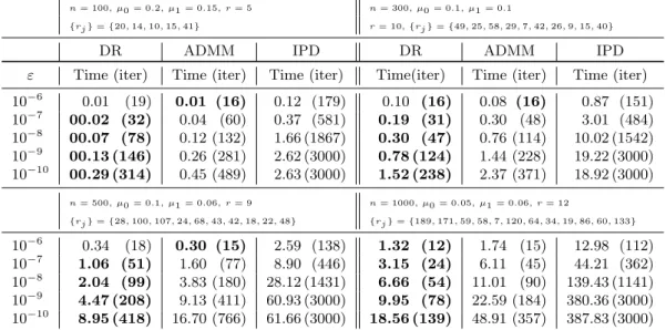
Table 5 allows us to compare the algorithms in terms of computation time (in seconds) and iteration number (averaged on 8 noise realizations, where the shortest and the longest times among the 10 runs were discarded), for the four scenarios corresponding to distinct problem sizes and block distributions. It can be observed that the behaviors of ADMM and DR are similar, while IPD requires many more iterations and time to reach the same precision. Furthermore, the latter fails to reach a high precision in the allowed maximum number of iterations, for all the four examples. The main source of computational cost of each procedure lies in the eigenvalue decomposition of a matrix, hence one iteration of any procedure among DR, ADMM and IPD takes approximately the same amount of time, which mainly depends on the matrix dimension. Furthermore, Table 5 shows that the DR approach often requires less iterations to achieve the same precision level, hence reaching a lower computational cost with respect to the other two procedures.

Table 5: Comparison in terms of convergence time between DR, ADMM and IPD procedures. The enlighten times refer to the shortest ones. Among the 10 realization, the shortest and the longest timings were discarded in the computation of the arithmetic mean.

n= 100, µ0 = 0.2, µ1 = 0.15, r= 5 n= 300, µ0 = 0.1, µ1 = 0.1

{rj}={20,14,10,15,41} r= 10,{rj}={49,25,58,29,7,42,26,9,15,40}

DR ADMM IPD DR ADMM IPD

ε Time (iter) Time (iter) Time (iter) Time(iter) Time (iter) Time (iter)

10−6 0.01 (19) 0.01 (16) 0.12 (179) 0.10 (16) 0.08 (16) 0.87 (151) 10−7 _{00.02 (32) 0.04 (60) 0.37 (581) 0.19 (31) 0.30 (48) 3.01 (484)} 10−8 00.07 (78) 0.12 (132) 1.66 (1867) 0.30 (47) 0.76 (114) 10.02 (1542) 10−9 _{00.13 (146) 0.26 (281) 2.62 (3000) 0.78 (124) 1.44 (228) 19.22 (3000)} 10−10 00.29 (314) 0.45 (489) 2.63 (3000) 1.52 (238) 2.37 (371) 18.92 (3000) n= 500, µ0 = 0.1, µ1 = 0.06, r= 9 n= 1000, µ0 = 0.05, µ1 = 0.06, r= 12 {rj}={28,100,107,24,68,43,42,18,22,48} {rj}={189,171,59,58,7,120,64,34,19,86,60,133} 10−6 0.34 (18) 0.30 (15) 2.59 (138) 1.32 (12) 1.74 (15) 12.98 (112) 10−7 _{1.06 (51) 1.60 (77) 8.90 (446) 3.15 (24) 6.11 (45) 44.21 (362)} 10−8 2.04 (99) 3.83 (180) 28.12 (1431) 6.66 (54) 11.01 (90) 139.43 (1141) 10−9 _{4.47 (208) 9.13 (411) 60.93 (3000) 9.95 (78) 22.59 (184) 380.36 (3000)} 10−10 8.95 (418) 16.70 (766) 61.66 (3000) 18.56 (139) 48.91 (357) 387.83 (3000)

5.2. Application to Robust Graphical Lasso

Let us now apply the MM approach presented in Section 4.3 to the problem of precision matrix estimation introduced in (30) on synthetic and real–world datasets.

Precision matrix estimation. A sparse precision matrixC∗of dimensionn×nis randomly created, where the number of non–zero entries is chosen as a proportionp∈]0,1[ of the total numbern2_{. Then,N realizations}

(x(i)₎

1≤i≤N of a Gaussian multivalued random variable with zero mean and covarianceY∗ = (C∗)−1 are

generated. Gaussian noise with zero mean and covariance σ2Id, σ > 0, is finally added to the x(i)’s, so

0.1 0.2 0.3 0.4 0.5 0.6 0.7 0.8 Noise level σ 0.1 0.2 0.3 0.4 0.5 0.6 0.7 0.8 0.9 1 rmse MM DR GLASSO

(a) Behaviour of rmse wrtσ.

0.1 0.2 0.3 0.4 0.5 0.6 0.7 0.8 Noise level σ 0 0.05 0.1 0.15 0.2 0.25 0.3 0.35 0.4 0.45 fpr MM DR GLASSO (b) Behaviour of fpr wrtσ.

Figure 2: Estimation results for different noise levels in terms ofrmse(upper panel) andfpr(lower panel) for MM, GLASSO and DR approaches. The MM procedure has a stable behaviour wrt to increasing noise, while DR and GLASSO strongly suffer from the presence of noise.

in Section 4.1, the estimation ofC∗ can be performed by using the MM algorithm from Section 4.3 based on the minimization of the nonconvex cost (30) with regularization functions g1 = µ1k · k1, µ1 > 0, and

(∀C∈ S++

n )g0(C) =µ0R1 C−1

,µ0>0. The computation of proxγ(ϕ+ψ)withγ∈]0,+∞[ related to this

particular choice forg0 and functionϕgiven by (36) and (34) leads to the search of the only positive root

of a polynomial of degree 4.

A synthetic dataset of sizen= 100 is created, where matrixC∗has 20 off-diagonal non-zero entries (i.e.,

p = 10−3_{) and the corresponding covariance matrix has condition number 0.125. N = 1000 realizations}

are used to compute the empirical covariance matrixS. In our MM algorithm, the inner stopping criterion (line 7 in Algorithm 2) is based on the relative difference of majorant function values with a tolerance of 10−10, while the outer cycle is stopped when the relative difference of the objective function values falls below 10−8. The DR algorithm is used to solve the inner subproblems, by using parameters (∀`)

γ` = 1, (∀k) α`,k = 1 (see Algorithm 2, lines 4–13). The allowed maximum inner (resp. outer) iteration number is 2000 (resp. 20). The quality of the results is quantified in terms of fpr (false positive rate) on the precision matrix and rmse(relative mean square error) with respect to the true covariance matrix. The parameters µ1 and µ0 are set in order to obtain the best reconstruction in terms of rmse. For eight

values of the noise standard deviationσ, Fig. 2 illustrates the reconstruction quality (averaged on 20 noise realizations) obtained with our method, as well as two convex minimization approaches that do not take into account the noise in their formulation, namely the classical GLASSO approach from [74], code available

athttp://stanford._{edu/~boyd/papers/admm/covsel/covsel example}.html, which amounts to solve (1)

12.2712.2812.3012.3112.3212.3312.34

Computational time (secs)

0 1000 2000 3000 4000 5000 6000 7000 8000 Objective function Outer MM iteration Inner DR iteration (a) MM 0 0.5 1 1.5 2 2.5 3 3.5 4 4.5

Computational time (secs) 0 2000 4000 6000 8000 10000 12000 Objective function (b) DR 0.01 0.02 0.03 0.04 0.05 0.06 0.07 0.08 0.09

Computational time (secs) 76 78 80 82 84 86 88 90 92 Objective function (c) GLASSO

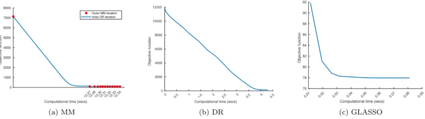
Figure 3: Evolution of the objective functions of each tested method whenσ= 0.5. The GLASSO approach has the fastest rate, but on the other hand it provides no reliable results. The major cost of the MM procedure lies in the first iteration, while the other iterations are fast.

(1) withf =−log det, (∀C∈ S++

n )g(C) =µ0R1 C−1+µ1kCk1. For the DR approach, proxγ(ϕ+ψ)with γ∈]0,+∞[ is given by the fourth line of Table 2 (whenp= 1).

As expected, as the noise variance increases the reconstruction quality deteriorates. The GLASSO procedure is strongly impacted by the presence of noise, whereas the MM approach achieves better results, also when compared with DR algorithm. Moreover, the MM algorithm significantly outperforms both other methods in terms of support reconstruction, revealing itself very robust with respect to an increasing level of noise. Fig. 3 depicts the behavior of the objective function of each of the three compared methods, for the problem instance whenσ= 0.5, as a function of the computational time.

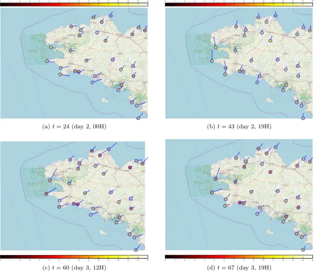
Mol`ene Dataset. We now consider a real dataset consisting of weather information collected by 55 stations of Radome type located in a French region between 47°N and 49°N, and 2°W and 6°W. The data refer to the Archipel Mol`ene project and they were collected from 1st Jan 2014 to 31st Jan 2014. They contain hourly information about rain (precipitation in kg/m2), temperature (value, maximal temperature of air, minimal temperature of air) and wind (speed [10’ mean], max speed [10’ mean], max speed [m/s]; direction [10’ mean], max direction [10’ mean], max direction [angle]): this dataset is freely available2_{, a visualization}

of four snapshots of these data is shown in Fig. 4. In this experiment the focus is on speed and direction of the wind: the collected data are stored in two matrices Wd and Ws both belonging to R31×744, i.e.

the hourly registrations (744 = 24×31) were taken by 31 (over 55) weather stations. The interest lies in finding connections between the different spots. The time interval considered in the whole dataset is quite large, it covers an entire month and then it can masquerade some interactions, so that only a subset referring to the first 3 days is retained. We also discarded the records from the weather station with code name PLOUDALMEZEAU as there were presenting erroneous and/or missing values. This pre-processing

2_{https://www.data.gouv.}

1 2 3 4 5 6 7 8 9 10 11 12 13 14 15 16 17 18 19 20 21 22 23 24 25 26 27 28 29 30 0 1 2 3 4 5 6 7 8 9 10 11 12 13 14 15 (a)t= 24 (day 2, 00H) 1 2 3 4 5 6 7 8 9 10 11 12 13 14 15 16 17 18 19 20 21 22 23 24 25 26 27 28 29 30 0 1 2 3 4 5 6 7 8 9 10 11 12 13 14 15 (b)t= 43 (day 2, 19H) 1 2 3 4 5 6 7 8 9 10 11 12 13 14 15 16 17 18 19 20 21 22 23 24 25 26 27 28 29 30 0 1 2 3 4 5 6 7 8 9 10 11 12 13 14 15 (c)t= 60 (day 3, 12H) 1 2 3 4 5 6 7 8 9 10 11 12 13 14 15 16 17 18 19 20 21 22 23 24 25 26 27 28 29 30 0 1 2 3 4 5 6 7 8 9 10 11 12 13 14 15 (d)t= 67 (day 3, 19H)

Figure 4: Visualization of some snapshots ofMol`eneDataset. Each point represents a weather station (see Fig. 5 for stations’ names). The blue arrows represent wind direction and their length is proportional to wind speed. The color of each station refers to the recorded temperature (in°C). The map shows the French region between 47°N and 49°N and 2°W and 6°W and was downloaded fromopenstreetmap.org.

procedure leads to smaller matrices (Wd,Ws)∈(R30×72)2, i.e. n= 30 andN = 72. We propose to consider

the wind data regarding both speed and direction in a coupled manner: a new data matrixWds=WdWs

is considered. In this way, the direction of the wind is modulated by its speed. Matrix Sin Algorithm 2 is taken as S = DS1, S ∈ R30×30, where S1 is the empirical covariance of the rows in Wds and D

is a symmetric matrix which encodes the relative distances in kilometers between the weather stations:

di,j= (0.1)

ri,j_{, wherer}

i,j is the distance between thei–th and the j–th stations, andri,i= 0 for everyi.

We apply the proposed MMDR algorithm for minimizing (30) withg0=µ0R1 (·)−1

andg1=µ1k · k1.

The noise level σis set to the standard deviation of the elements in Wds. Further setting of Algorithm 2

loop toleranceεo= 10−4 (maximum 20 iterations). The results are depicted in Fig. 5.

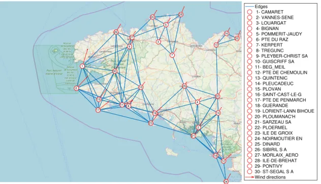
Within these settings, the graph is sparse, easy to interpret (cf. Fig. 5). Moreover, a three–subgraphs structure arises: the bigger subgraph is located in the west part, connected to the eastern one by the nodes 19 and 23. In the north a group of 5 stations (3, 5, 7, 20 and 28) depicts a subgraph which shares edges with the other twos. Finally, three isolated stations are connected in the north–east part of the map.

1 2 3 4 5 6 7 8 9 10 11 12 13 14 15 16 17 18 19 20 21 22 23 24 25 26 27 28 29 30 1 2 3 4 5 6 7 8 9 10 11 12 13 14 15 16 17 18 19 20 21 22 23 24 25 26 27 28 29 30 Edges 1- CAMARET 2- VANNES-SENE 3- LOUARGAT 4- BIGNAN 5- POMMERIT-JAUDY 6- PTE DU RAZ 7- KERPERT 8- TREGUNC 9- PLEYBER-CHRIST SA 10- GUISCRIFF SA 11- BEG_MEIL 12- PTE DE CHEMOULIN 13- QUINTENIC 14- PLEUCADEUC 15- PLOVAN 16- SAINT-CAST-LE-G 17- PTE DE PENMARCH 18- GUERANDE 19- LORIENT-LANN BIHOUE 20- PLOUMANAC'H 21- SARZEAU SA 22- PLOERMEL 23- ILE DE GROIX 24- NOIRMOUTIER EN 25- DINARD 26- SIBIRIL S A 27- MORLAIX_AERO 28- ILE-DE-BREHAT 29- PONTIVY 30- ST-SEGAL S A Wind directions

Figure 5: Recovered graph from wind direction–speed data. Three main subgraphs are present, in the west, in the north and in the south–east. A small group of three stations is connected in the far north. The red arrows represent medium wind direction modulated by the medium speed in the considered time interval.

We now perform comparisons with respect to the classical GLASSO approach, and to the case when

σ is assumed to be 0. We apply Douglas-Rachford algorithm for minimizing Eq. (1) with f =−log det, (∀C∈ S++

n )g(C) =µ0R1 C−1

+µ1kCk1. Two settings are considered for the parameters (µ0, µ1), namely

(0,5×10−6_{) corresponding to GLASSO and (µ}

0, µ1) = (6×10−3,10−4). The algorithm parameters are γ` ≡ 4, α(`,k) ≡ 1.8, and the stopping criterion tolerance is 10−6 with a maximum number of 4×104

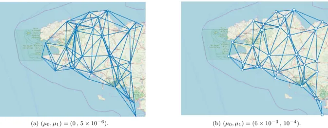
iterations. The recovered graphs are depicted in Fig. 6. The GLASSO graph seems to provide no useful information, since the degree of the nodes stays rather high. For the second setting of parameters, here-again, the graph does not show any particular structure. Those comparisons illustrate the advantage of our MMDR method, both accounting for the presence of noise and introducing a spectral penalization.

(a) (µ0, µ1) = (0,5×10−6). (b) (µ0, µ1) = (6×10−3,10−4).

Figure 6: DR algorithm for minimizing (1) withf = −log det and (∀C ∈ S++

n )g(C) =µ0R1 C−1

+µ1kCk1, for two

different settings of regularization parameters.

6. Conclusions

In this work, various proximal tools have been introduced to deal with optimization problems involving real symmetric matrices. We have focused on the variational framework (1) which is closely related to the computation of a proximity operator with respect to a Bregman divergence. It has been assumed thatf in (3) is a convex spectral function, andgreads asg0+g1, whereg0is a spectral function. We have provided a fully spectral solution in Section 2 wheng1≡0, and, in particular, Corollary 1 could be useful for developing algorithms involving proximity operators in other metrics than the Frobenius one. Wheng16≡0, a proximal iterative approach has been presented, which is grounded on the use of the Douglas–Rachford procedure. As illustrated by the lists of proximity operators provided for a wide range of choices forf andg0, the main advantage of the proposed algorithm is its great flexibility. Numerical experiments show its superiority in terms of convergence speed with respect to two state–of–art algorithms solving the same problem. The proposed matrix estimation framework has also allowed us to introduce a nonconvex formulation of the precision matrix estimation problem arising in the context of noisy graphical lasso. The nonconvexity of the obtained objective function has been circumvented through an MM approach, each step of which consists of solving a convex problem by a Douglas-Rachford sub-iteration. Comparisons with state–of–the–art solutions have demonstrated the robustness of the proposed method. The proposed model and the MM procedure devoted to the minimization of the non–convex functional also reveals to be useful for analyzing real–world multivariate time series from meteorology. It is worth mentioning that all the results presented in this paper could be easily extended to complex Hermitian matrices. It would also be interesting to perform a deeper statistical analysis of the performance of the robust GLASSO approach proposed in this paper.

Appendix A.

Proof of Theorem 2. (i) Since it has been assumed thatf andg0are spectral functions, we have

(∀C∈ Sn) f(C) +g0(C) =ϕ(d) +ψ(d), (A.1)

where d ∈ Rn is a vector of the eigenvalues of C. It can be noticed that minimizing (12) is obviously

equivalent to minimizefe−γ−1trace (C+γT

·) +g0 wherefe=f+k · k2_F/(2γ). Then

e

f(C) =ϕ_e(d), (A.2)

whereϕ_e=ϕ+k · k2_{/(2γ). Since we have assumed thatϕ∈Γ}

0(Rn),ϕeis proper, lower-semicontinuous, and strongly convex. Asψ is lower bounded by an affine function, it follows that

d7→ϕ_e(d)−γ−1λ>d+ψ(d) (A.3) is lower bounded by a strongly convex function and it is thus coercive. In addition, domϕ_e= domϕ, hence domϕ_e∩domψ6=_∅. Let us now apply Theorem 1. Let λb be a minimizer of (A.3). It can be claimed that

b

C=UDiag(bλ)U> is a minimizer of (12). On the other hand, minimizing (A.3) is equivalent to minimize

γ(ϕ+ψ) +1₂k · −λk2_{, which shows that}

b

λ∈Proxγ(ϕ+ψ)(λ).

(ii) If ψ ∈ Γ0(Rn), then it is lower bounded by an affine function [45, Theorem 9.20]. Furthermore,

ϕ+ψ∈Γ0(Rn) and the proximity operator ofγ(ϕ+ψ) is thus single valued. On the other hand, we also

have γ(f −trace (T·) +g0) ∈ Γ0(Sn) [75, Corollary 2.7], and the proximity operator of this function is

single valued too. The result directly follows from (i).

Appendix B.

Proof of Lemma 2. By using differential calculus rules in [76], we will show that the Hessian of −TS

evaluated at any matrix in S++

n is a positive semidefinite operator. In order to lighten our notation, for

every invertible matrix C, let us define M=C−1_+σ2_I

d. Then, the first-order differential ofTS at every

C∈ S++ n is d trace (TS(C)) = trace dM−1 S = trace −M−1(dM)M−1S = trace C−1+σ2Id −1 S C−1+σ2Id −1 C−1(dC)C−1 = trace Id+σ2C −1 S Id+σ2C −1 (dC). (B.1)

We have used the expression of the differential of the inverse [76, Chapter 8, Theorem 3] and the invariance of the trace with respect to cyclic permutations. It follows from (B.1) that the gradient ofTSreads

(∀C∈ S++ n ) ∇TS(C) = Id+σ2C −1 S Id+σ2C −1 . (B.2)

In order to calculate the HessianHof TS, we calculate the differential of∇TS. Again, in order to simplify

our notation, for every matrixC, we define

N= Id+σ2C ⇒ dN=σ2dC. (B.3)

The differential of∇TSat everyC∈ Sn++ then reads

d vect (∇TS(C)) = vect d(N−1SN−1) = vect (dN−1)SN−1+N−1(dSN−1) = −vect(N−1(dN)N−1SN−1)−vect N−1SN−1(dN)N−1 = − N−1SN−1> ⊗N−1vect(dN) + − N−1> ⊗N−1SN−1d vect(N) = − N−1SN−1 ⊗N−1+N−1⊗ N−1SN−1 vect(dN) = H(C) d vect(C) with H(C) =−σ2∇TS(C)⊗ Id+σ2C −1 + Id+σ2C −1 ⊗ ∇TS(C) . (B.4)

To derive the above expression, we have used the facts that, for everyA∈_Rn×m_,X∈

Rm×p, andB∈Rp×q,

vect (AXB) = B>⊗A

vectX[76, Chapter 2,Theorem 2] and that matricesN andSare symmetric. Let us now check that, for every C ∈ S++

n , H(C) is negative semidefinite. It follows from expression

(B.2), the symmetry ofC, and the positive semidefiniteness ofSthat∇TS(C) belongs toSn+. Since

∇TS(C)⊗ Id+σ2C −1> = ∇TS(C) > ⊗ Id+σ2C −1> =∇TS(C)⊗ Id+σ2C −1 , ∇TS(C)⊗ Id+σ2C −1

is symmetric. Let us denote by (γi)1≤i≤n ∈[0,+∞[n the eigenvalues of∇TS(C)

and by (ζi)1≤i≤n ∈ [0,+∞[n those of C. According to [76, Chapter 2, Theorem 1], the eigenvalues of ∇TS(C)⊗ Id+σ2C

−1

are γi/(1 +σ2_ζj)

1≤i,j≤n and they are therefore nonnegative. This allows us to

claim that ∇TS(C)⊗ Id+σ2C

−1

belongs toS_n+2. For similar reasons, Id+σ2C

−1

⊗ ∇TS(C) ∈ S_n+2, which allows us to conclude that−H(C) ∈ S_n+2. Hence, we have proved that TS is concave on Sn++. By

continuity ofTS relative toSn+, the concavity property extends onSn+.

Appendix C.

Proof of Theorem 5. First note that (C(`))`≥0 is properly defined by (38) since, for every C ∈ Sn++,

G(· |C) is a coercive lower-semicontinuous function. It indeed majorizesFwhich is coercive, sincef+g0+g1

(i) As a known property of MM strategies, F(C(`)₎

`≥0is a decaying sequence [69]. Under our assumptions,

we have already seen that F has a minimizer. We deduce that F(C(`)₎

`≥0 is lower bounded, hence

convergent.

(ii) Since F(C(`)₎

`≥0is a decaying sequence, (∀`≥0)C

(`)_{∈E. SinceF is proper, lower-semicontinuous,}

and coercive,E is a nonempty compact set and (C(`)₎

`≥0admits a cluster point in E.

(iii) IfCb is a cluster point of (C(`))`≥0, then there exists a subsequence (C(`k))k≥0converging toCb. SinceE is a nonempty subset of the relative interior of domg0∩domg1 andg0+g1∈Γ0(Sn),g0+g1is continuous

relative to E [45, Corollary 8.41]. As f +TS is continuous on domf ∩domTS = Sn++, F is continuous

relative toE. Hence, Fb = limk→+∞F(C(`k)) =F(bC). On the other hand, by similar arguments applied to sequence (C(`k+1)₎

k≥0, there exists a subsequence (C(`kq+1))q≥0 converging to some Cb0 ∈E such that b

F=F(Cb0). In addition, thanks to (38), we have

(∀C∈ Sn)(∀q∈N) G(C(`kq+1)|C(`kq))≤ G(C|C(`kq)). (C.1)

By continuity off and∇TS onSn++ and by continuity ofg0+g1 relative toE,

(∀C∈ Sn) G(Cb0|Cb)≤ G(C|Cb). (C.2) Let us now suppose thatCb is not a critical point ofF. Since the subdifferential ofG(· |Cb) atCb is∇f(Cb) + ∇TS(bC) +∂(g0+g1)(Cb) [45, Corollary 16.48(ii)], the null matrix does not belong to this subdifferential, which means thatCb is not a minimizer ofG(· |Cb) [45, Theorem 16.3]. It follows from (C.2) and standard MM properties thatF(Cb0)≤ G(Cb0 |Cb)<G(Cb |Cb) =F(Cb). The resulting strict inequality contradicts the

already established fact thatF(Cb0) =F(bC).

References

[1] J. C. Duchi, S. Gould, D. Koller, Projected Subgradient Methods for Learning Sparse Gaussians, in: UAI 2008, Proceedings of the 24th Conference in Uncertainty in Artificial Intelligence, Helsinki, Finland, July 9-12, 2008, 2008, pp. 145–152. [2] S. Ma, L. Xue, H. Zou, Alternating direction methods for latent variable Gaussian graphical model selection, Neural

Comput. 25 (8) (2013) 2172–2198.doi:10.1162/NECO a 00379.

[3] O. Banerjee, L. El Ghaoui, A. d’Aspremont, Model selection through sparse maximum likelihood estimation for multivari-ate Gaussian or binary data, J. Mach. Learn. Res. 9 (2008) 485–516.

[4] V. Chandrasekaran, P. A. Parrilo, A. S. Willsky, Latent variable graphical model selection via convex optimization, Ann. Statist. 40 (4) (2012) 1935–1967. doi:10.1214/11-AOS949.

[5] J. Guo, E. Levina, G. Michailidis, J. Zhu, Joint estimation of multiple graphical models, Biometrika 98 (1) (2011) 1.

doi:10.1093/biomet/asq060.

[6] J. Friedman, T. Hastie, R. Tibshirani, Sparse inverse covariance estimation with the graphical LASSO, Biostatistics 9 (3) (2008) 432–441.doi:10.1093/biostatistics/kxm045.

[7] A. Dempster, Covariance selection, Biometrics 28 (1972) 157–175.

[8] A. d’Aspremont, O. Banerjee, L. E. Ghaoui, First-order methods for sparse covariance selection, SIAM J. Matrix Anal. Appl. 30 (1) (2008) 56–66. doi:10.1137/060670985.

[9] J. Bien, R. J. Tibshirani, Sparse estimation of a covariance matrix, Biometrika 98 (4) (2011) 807–820.

[10] Y. Sun, P. Babu, D. P. Palomar, Robust estimation of structured covariance matrix for heavy-tailed elliptical distributions, IEEE Trans. Signal Process. 64 (14) (2016) 3576–3590.

[11] A. Wiesel, Unified framework to regularized covariance estimation in scaled Gaussian models, IEEE Trans. Signal Process. 60 (1) (2012) 29–38. doi:10.1109/TSP.2011.2170685.

[12] Y. Sun, P. Babu, D. P. Palomar, Regularized robust estimation of mean and covariance matrix under heavy tails and outliers, in: 2014 IEEE 8th Sensor Array and Multichannel Signal Processing Workshop (SAM), 2014, pp. 125–128.