Monte Carlo study of some classification-based ridge parameter estimators

(1)

Volume 16 | Issue 1

Article 24

5-1-2017

Monte Carlo Study of Some Classification-Based

Ridge Parameter Estimators

Adewale Folaranmi Lukman

Ladoke Akintola University of Technology

Kayode Ayinde

Ladoke Akintola University of Technology

Adegoke S. Ajiboye

Federal University of Technology

Follow this and additional works at:

http://digitalcommons.wayne.edu/jmasm

Part of the

Applied Statistics Commons,

Social and Behavioral Sciences Commons, and the

Statistical Theory Commons

This Regular Article is brought to you for free and open access by the Open Access Journals at DigitalCommons@WayneState. It has been accepted for

inclusion in Journal of Modern Applied Statistical Methods by an authorized editor of DigitalCommons@WayneState.

Recommended Citation

Lukman, A. F., Ayinde, K., & Ajiboye, A. S. (2017). Monte Carlo study of some classification-based ridge parameter estimators.

Journal of Modern Applied Statistical Methods, 16(1), 428-451. doi: 10.22237/jmasm/1493598240

(2)

Adewale Folaranmi Lukman is a teaching assistant in the Department of Statistics. Email

at

. Prof. Kayode Ayinde is a lecturer in the Department of

Statistics. Email at

. Dr. Ajiboye S. Adegoke is a lecturer in the

Department of Statistics.

Monte Carlo Study of Some

Classification-Based Ridge Parameter Estimators

A. F. Lukman

Ladoke Akintola Univ. of Technology Ogbomosho, Nigeria

K. Ayinde

Ladoke Akintola Univ. of Technology Ogbomosho, Nigeria

A. S. Ajiboye

Federal University of Technology Akure, Nigeria

Ridge estimator in linear regression model requires a ridge parameter, K, of which many

have been proposed. In this study, estimators based on Dorugade (

2014

) and Adnan et al.

(

2014

) were classified into different forms and various types using the idea of Lukman

and Ayinde (

2015

). Some new ridge estimators were proposed. Results shows that the

proposed estimators based on Adnan et al. (

2014

) perform generally better than the

existing ones.

Keywords:

linear regression model, multicollinearity, ridge estimator, mean square

error

Introduction

The parameter estimates obtained through the use of the Ordinary Least Squares

(OLS) estimator have optimal performance when there is no violation of any of

the assumptions of the classical linear regression model. One of the most basic of

these assumptions is that explanatory variables are independent. Multicollinearity

refers to the presence of strong or perfect linear relationships among the

explanatory variables. Multicollinearity is an inherent phenomenon in most

economic relationships due to the nature of economic magnitude (

Koutsoyiannis,

2003

). When there is a perfect relationship among the explanatory variables, the

regression coefficients of the OLS estimator are indeterminate, and the standard

error of the estimates becomes very large. Also, when there are strong

relationships among the explanatory variables, the regression estimates are

determinate but possesses large standard error (

Koutsoyiannis, 2003

).

(3)

Generally, the performance of OLS estimator is unsatisfactory when there is

multicollinearity (

Koutsoyiannis, 2003

). Several techniques have been suggested

in the literature to handle this problem. Massy (

1965

) introduced the principal

component regression to eliminate the model instability and reduce the variances

of the regression coefficients. Wold (

1966

) developed the partial least square to

deal with the problem of multicollinearity. Hoerl and Kennard (

1970

) proposed

the ridge estimator for dealing with multicollinearity in a regression model, which

modifies the OLS to allow biased estimation of the regression coefficients. This

study is limited to the application of the ridge regression estimator in handling the

problem of multicollinearity. Ridge estimator is defined as:





1

ˆ

_KI

R

X X

X Y



_



_





(1)

where K is a non-negative constant known as ridge parameter and I denotes

an identity matrix. When K equals zero, (

1 ) returns to OLS estimator; this is

defined as follows:





1

ˆ

OLS

X X

X Y



_



_



(2)

The corresponding mean square error (MSE) of (

1 ) and (

2 ) are defined

respectively as:

 









2 2 2 2 2 1 1

ˆ

_ˆ

ˆ

p _i p _i R _i _i i i

MSE

K









 







(3)

 

2 1

1 ˆ

_ˆ

p OLS _i i

MSE











(4)

where

λ

1

,

λ

2

, …,

λ

p

are the eigenvalues of

X'X

,

K

ˆ

is the estimator of the

ridge parameter K and



ˆ

_i

is the

i

th

_{element of the vector}



ˆ

_.

Although this estimator is biased, it gives a smaller mean squared error

when compared to the OLS estimator for a positive value of K (

Hoerl and

Kennard, 1970

). The use of the estimator depends largely on the ridge parameter,

K. Several methods for estimating this ridge parameter have been proposed by

different authors, as follows: Hoerl and Kennard (

1970

); McDonald and

(4)

Galarneau (

1975

); Lawless and Wang (

1976

); Hocking et al. (

1976

); Wichern and

Churchill (

1978

); Gibbons (

1981

); Nordberg (

1982

); Kibria (

2003

), Khalaf and

Shukur (

2005

), Alkhamisi et al. (

2006

), Muniz and Kibria (

2009

), Mansson et al.

(

2010

), Dorugade (

2014

) and recently, Lukman and Ayinde (

2015

). The purpose

of this study is to classify the ridge parameters proposed by Dorugade (

2014

) and

Adnan et al. (

2014

) into different forms and various types. A simulation study is

conducted and the performances of the estimators is examined via mean square

error (MSE).

Model and Estimators

A linear regression model can be expressed in matrix form as:

X + U

Y





(5)

where

X

is an

n

×

p

matrix with full rank, Y is a

n

× 1 vector of dependent

variable,

β

is a

p

× 1 vector of unknown parameters, and U is the error term such

that E(U) = 0 and E(UU

'

) =

σ

2

_I

n

. The Ordinary Least Square (OLS) estimator of

β

is defined in (

2 ): Model (

5 ) can be written in canonical form. Suppose there exists

an orthogonal matrix Q such that

X'

Q

X

= Ʌ, where Ʌ = diag(

λ

1

,

λ

2

, …,

λ

p

) and

λ

1

,

λ

2

, …,

λ

p

are the eigenvalues of

X'X

. Substituting

α

= Q

'β

, model (

5 ) can be

written as:

Z + U

Y





(6)

where

Z'Z

= Ʌ.

Therefore, the ridge estimator of

α

can be defined as:





1

ˆ

_R

Z Z

KI

Z Y



_



_





(7)

The corresponding mean square error (MSE) is defined as:

 









2 2 2 2 2 1 1

ˆ

K

ˆ

K

p _i p _i R _i _i i i

MSE











 







(8)

(5)

where



ˆ

_i

is the

i

th

_{element of the vector}

_α

₌

_Q'β

_{. Hoerl and Kennard (}

₁₉₇₀

₎

defined the value of the ridge parameter K that minimizes the mean square error

as:

2 2

ˆ

ˆK

,

ˆ

i i







where

2 1 2 1

ˆ

n i

e

n

p



_







₍₉₎

Hoerl and Kennard (

1970

) proposed

2 HK 2

ˆ

ˆK

.

ˆ

i i







They suggested estimating ridge parameter by taking the maximum (Fixed

Maximum) of



i2

such that the estimator of K is:

 

2 FM HK 2

ˆ

ˆk

ˆ

max

_i







(10)

Hoerl et al. (

1975

) proposed a different estimator of K by taking the

Harmonic Mean of the ridge parameter K

HKi

. This estimator is given as:

2 HM HK ₂ 1

ˆ

ˆK

_p i i

p









(11)

Kibria (

2003

) proposed some new estimators of K by taking the geometric

mean, arithmetic mean and median (

p

≥ 3) of the ridge parameter K

HKi

. These

estimators are respectively defined as:





1 2 GM HK 2 1

ˆ

ˆK

ˆ

p p i i









(12)

2 AM HK 1 2

ˆ

1 ˆK

ˆ

p i i

p









(13)

(6)

2 M HK 2

ˆ

ˆK

Median

ˆ

_i











_

_





(14)

Furthermore, Muniz and Kibria (

2009

) proposed some estimators of K in the

form of the square root of the geometric mean of K

HK_i

and its reciprocal, the

median of the square root of K

HKi

and its reciprocal, and varying maximum of the

square root of K

HK_i

and its reciprocal. These estimators are respectively defined

as:





1 2 GMSR HK 2 1

ˆ

ˆK

ˆ

p p i i









(15)





1 GMRSR HK ₂ 2 1

1 ˆK

ˆ

p p i i









(16)

2 MSR HK 2

ˆ

ˆK

Median

ˆ

_i













_



_





(17)

MRSR HK ₂ 2

1 ˆK

Median

ˆ

_i



















_

_













(18)

2 VMSR HK 2

ˆ

ˆK

max

ˆ

_i













_



_





(19)

VMRSR HK ₂ 2

1 ˆK

max

ˆ

_i



















_

_













(20)

(7)

Dorugade (

2014

) suggested the modification of the generalized ridge

parameter in (

9 ) by multiplying the denominator with λ

max

/2. The estimator is

defined as:

2 D 2 max

2 ˆk

ˆ

_i



 



(21)

where

λ

max

is the maximum eigenvalue of

X'X

.

Following Kibria (

2003

), Dorugade (

2014

) suggested the following ordinary

ridge regression for the ridge parameter in (

21 ).

2 HM D ₂ max 1

ˆ

2 ˆK

ˆ

p i i

p





_







(22)

2 M D 2 max

ˆ

2 ˆK

Median

ˆ

_i



 







_

_





(23)





1 2 GM D 2 max ₁

ˆ

2 ˆK

ˆ

p p i i





_







(24)

2 AM HK 1 2 max

ˆ

2

1 ˆK

ˆ

p i i

p













(25)

Following Dorugade (

2014

), Adnan et al. (

2014

) proposed some ridge

parameters:

2 HM 1 ₂ max ₁

ˆ

5 ˆK

ˆ

N p i i

p





_







(26)

2 HM 2 ₂ max ₁

ˆ

ˆK

ˆ

N p i i

p





_







(27)

(8)

 

1 4 2 HM 3 ₂ 1 1

ˆ

2 ˆK

ˆ

N p p i i i i

p







 





(28)

2 HM 4 2 1 1

ˆ

2 ˆK

ˆ

N _p _p i i i i

p







 



 

(29)

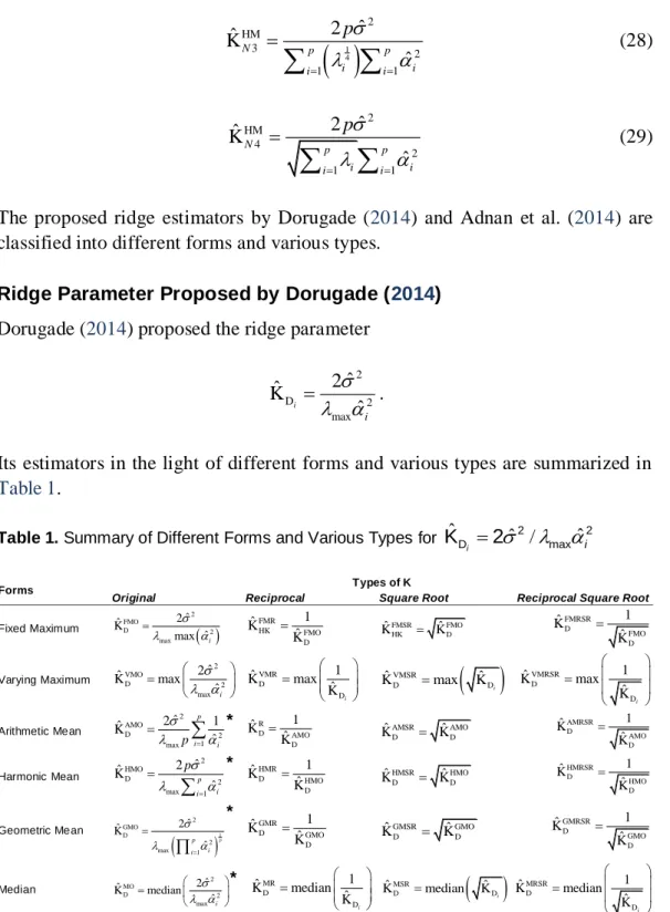
The proposed ridge estimators by Dorugade (

2014

) and Adnan et al. (

2014

) are

classified into different forms and various types.

Ridge Parameter Proposed by Dorugade (

2014

)

Dorugade (

2014

) proposed the ridge parameter

2 D 2 max

ˆ

2 ˆK

ˆ

i i



 



.

Its estimators in the light of different forms and various types are summarized in

Table 1

.

Table 1.

Summary of Different Forms and Various Types for

K

ˆ

_D



2   

ˆ /

2 _max

ˆ

2

i i

Forms Types of K

Original Reciprocal Square Root Reciprocal Square Root

Fixed Maximum

_{ }

2 FMO D 2 max ˆ 2 ˆK ˆ max i     FMR HK FMO D

1 ˆK

ˆK



FMSR FMO HK D ˆ ˆ K  K FMRSR D FMO D

1 ˆK

ˆK



Varying Maximum 2 VMO D 2 max

ˆ

2 ˆK

max

ˆ

_i



 







_

_





VMR D D

1 ˆK

max

ˆK

i









_



_





 

VMSR D D

ˆ

K

max

K

i



VMRSR D D

1 ˆK

max

ˆK

i











_

_





Arithmetic Mean 2 AMO D 2 1 max

ˆ

2

1 ˆK

ˆ

p i i

p













*

R D AMO D

1 ˆK

ˆK



AMSR AMO D D

ˆ

K



K

AMRSRD AMO D 1 ˆK ˆK  Harmonic Mean 2 HMO D ₂ max 1

ˆ

2 ˆK

ˆ

p i i

p





_







*

HMR D HMO D

1 ˆK

ˆK



HMSR HMO D D

ˆ

K



K

HMRSRD HMO D 1 ˆK ˆK  Geometric Mean





1 2 GMO D 2 max 1 ˆ 2 ˆK ˆ p p i i   _ 



*

GMR D GMO D

1 ˆK

ˆK



GMSR GMO D D

ˆ

K



K

GMRSRD GMO D

1 ˆK

ˆK



Median 2 MO D 2 max ˆ 2 ˆK median ˆi          

*

MR D D

1 ˆK

median

ˆK

i









_



_





 

MSR D D ˆ ˆ K median K i MRSR D D

1 ˆK

median

ˆK

i











_

_





(9)

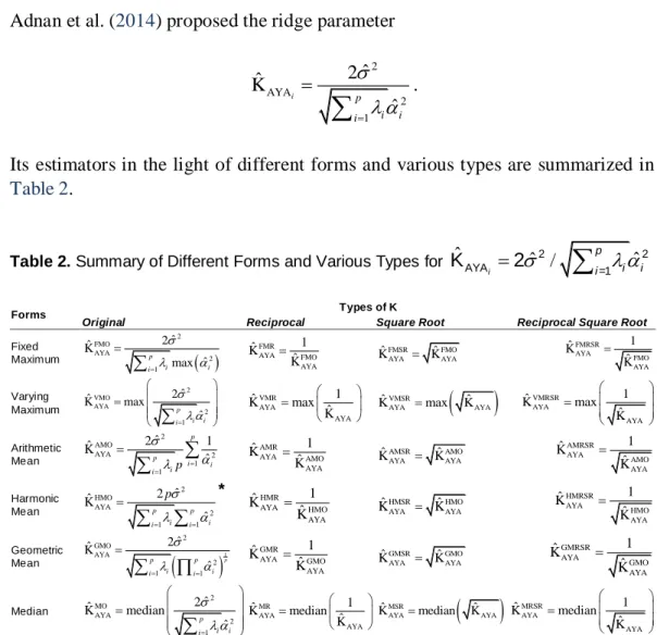
Ridge Parameter Proposed by Adnan et al. (

2014

)

Adnan et al. (

2014

) proposed the ridge parameter

2 AYA 2 1

ˆ

2 ˆK

ˆ

i _p i i i



 





.

Its estimators in the light of different forms and various types are summarized in

Table 2

.

Table 2.

Summary of Different Forms and Various Types for

ˆ

_AYA





ˆ /

2



 

ˆ

2

=1

K

2

i p i i i Forms Types of K

Original Reciprocal Square Root Reciprocal Square Root

Fixed Maximum

 

2 FMO AYA 2 1 ˆ 2 ˆK ˆ max p i i i







 



FMRAYA FMO AYA

1 ˆK

ˆK



FMSR FMO AYA AYA ˆ ˆ K  K FMRSR AYA FMO AYA 1 ˆK ˆK  Varying Maximum 2 VMO AYA 2 1 ˆ 2 ˆK max ˆ p i i i          _ _   



 VMR AYA AYA

1 ˆK

max

ˆK



















VMSR AYA AYA ˆ ˆ K max K VMRSRAYA AYA 1 ˆK max ˆK          Arithmetic Mean 2 AMO AYA 2 1 1

ˆ

2

1 ˆK

ˆ

p p i i i i

p







 





AMRAYA AMO AYA

1 ˆK

ˆK



AMSR AMO AYA AYA

ˆ

K



K

AMRSR AYA AMO AYA

1 ˆK

ˆK



Harmonic Mean 2 HMO AYA 2 1 1

ˆ

2 ˆK

ˆ

p p i i i i

p







 



 

*

_HMR AYA HMO AYA

1 ˆK

ˆK



HMSR HMO AYA AYA

ˆ

K



K

HMRSRAYA HMO AYA

1 ˆK

ˆK



Geometric Mean





1 2 GMO AYA 2 1 1 ˆ 2 ˆK ˆ p p p i i i i







  





GMR AYA GMO AYA

1 ˆK

ˆK



GMSR GMO AYA AYA

ˆ

K



K

GMRSR AYA GMO AYA

1 ˆK

ˆK



Median 2 MO AYA 2 1

ˆ

2 ˆK

median

ˆ

p i i i



 













_

_











MR AYA AYA

1 ˆK

median

ˆK



















MSR AYA AYA ˆ ˆ K median K MRSR AYA AYA 1 ˆK median ˆK         

Notes: * Adnan et al. (2014); all others are proposed estimators

The ridge parameter estimators in

Table 1

and

2 were examined and evaluated in

this study.

Monte Carlo Simulation

The considered regression model is of the form:

0 1 1 2 2

t i i p ip t

(10)

where

t

= 1, 2, …,

n

;

p

= 3, 7.

The error term

U

t

was generated to be normally distributed with mean zero

and variance

σ

2

_,

_U

t

~ N

(0,

σ

2

). In this study,

σ

were taken to be 0.5, 1 and 5.

β

0

was taken to be identically zero. When

p

= 3, the values of

β

were chosen

to be

β

= (0.8, 0.1, 0.6)

'

. When

p

= 7, the values of

β

were chosen to be

β

= (0.4, 0.1, 0.6, 0.2, 0.25, 0.3, 0.53)

'

. The parameter values were chosen such

that

β'β

= 1 which is a common restriction in simulation studies of this type

(

Muniz and Kibria, 2009

). We varied the sample sizes between 10, 20, 30, 40 and

50. Following McDonald and Galarneau (

1975

), Wichern and Churchill (

1978

),

Gibbons (

1981

), Kibria (

2003

), Muniz and Kibria (

2009

), Lukman and Ayinde

(

2015

), the explanatory variables were generated using the following equation:





1 2 2

1 ,

1, 2,3,..., ,

1, 2,..., .

ij ij ip

X

 



Z





Z

i



n j



p

(31)

where

Z

ij

is independent standard normal distribution with mean zero and

unit variance,

ρ

is the correlation between any two explanatory variables and

p

is

the number of explanatory variables. The number of explanatory variable (

p

) is

taken to be three (3) and seven (7). The value of

ρ

is taken as 0.95, 0.99

respectively. Three different values of

σ

, 0.5, 1 and 5, were also used. The

experiment is replicated 1,000 times. The ridge parameter estimators are

evaluated using mean square error (MSE).

Results

The results of the simulation are presented in

Table 3

and

4 . These tables provide

the results of the estimated mean square error of the ridge parameter when the

number of regressors is three (3) and seven (7) respectively. The mean square

error increases as the multicollinearity level increases. Across each

multicollinearity level, the mean square error decreases as the sample sizes

increase from 10 to 50, while increasing the number of regressors increases the

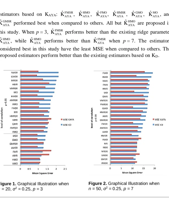
estimated MSE. However, it is observed that the ridge estimators based on K

AYA

performed consistently better than K

D

. Occasionally, this method performs better

than K

AYA

. For instance, estimators

ˆK

VMSRD

and

AMSR D

ˆK

perform consistently well

over estimators based on K

AYA

especially when the number of regressors

increases to seven (7), and when the number of regressors is three (3), especially

when

n

≤ 20. This can be seen in

Figure 1

and

2 . The following ridge parameter

(11)

estimators based on K

AYA

:

ˆK

FMSRAYA

,

HMO AYA

ˆK

,

ˆK

FMO_AYA

,

ˆK

HMSR_AYA

,

ˆK

GMO_AYA

,

ˆK

MO_AYA

,

and

GMSR

AYA

ˆK

performed best when compared to others. All but

ˆK

HMO_AYA

are proposed in

this study. When

p

= 3,

ˆK

FMSR_AYA

performs better than the existing ridge parameter

HMO AYA

ˆK

,

while

ˆK

HMO_AYA

performs better than

ˆK

FMSR_AYA

when

p

= 7. The estimators

considered best in this study have the least MSE when compared to others. The

proposed estimators perform better than the existing estimators based on K

D

.

Figure 1.

Graphical Illustration when

n

= 20,

σ

2

_{= 0.25,}

_p

_{= 3}

Figure 2.

Graphical Illustration when

n

= 50,

σ

2

_{= 0.25,}

_p

_{= 7}

(12)

Table 3.

Estimated Mean Square Error of ridge parameter when

p

= 3

p = 3, σ = 0.5, ρ = 0.95

n = 10 n = 20 n = 30 n = 40 n = 50

Methods ˆ

D

K KÂYA K ˆD KÂYA K ˆD KÂYA K ˆD KÂYA K ˆD KÂYA FMO 3.501 2.297 1.757 1.265 1.633 1.224 0.877 0.750 0.680 0.611 FMR 4.470 4.049 2.091 1.683 2.149 1.722 1.191 0.795 1.017 0.631 FMSR 2.340 1.757 1.369 1.004 1.309 0.941 0.789 0.627 0.635 0.532 FMRSR 3.904 3.550 1.630 1.363 1.690 1.390 0.805 0.595 0.649 0.456 VMO 2.374 2.263 1.248 1.078 1.235 1.039 0.705 0.572 0.581 0.471 VMR 4.470 4.049 2.091 1.683 2.149 1.722 1.191 0.795 1.017 0.631 VMSR 2.004 2.289 1.019 0.969 1.000 0.948 0.607 0.493 0.514 0.407 VMRSR 3.904 3.550 1.630 1.363 1.690 1.390 0.805 0.595 0.649 0.456 AMO 2.589 2.033 1.358 1.019 1.337 0.987 0.755 0.571 0.611 0.477 AMR 4.092 3.659 1.856 1.575 1.889 1.532 1.016 0.760 0.843 0.592 AMSR 1.995 2.088 1.079 0.932 1.054 0.906 0.652 0.506 0.546 0.426 AMRSR 3.532 3.107 1.465 1.293 1.490 1.242 0.725 0.630 0.572 0.500 HMO 3.184 1.863 1.665 1.045 1.579 1.027 0.865 0.666 0.674 0.559 HMR 4.322 3.889 1.968 1.573 2.037 1.606 1.102 0.724 0.938 0.568 HMSR 2.098 1.723 1.259 0.920 1.215 0.868 0.759 0.575 0.618 0.494 HMRSR 3.789 3.380 1.548 1.287 1.614 1.302 0.754 0.574 0.602 0.448 GMO 2.782 1.762 1.483 0.919 1.447 0.903 0.821 0.562 0.651 0.476 GMR 4.206 3.747 1.892 1.546 1.956 1.535 1.043 0.730 0.882 0.571 GMSR 1.963 1.855 1.142 0.883 1.109 0.845 0.709 0.521 0.588 0.447 GMRSR 3.665 3.215 1.489 1.260 1.546 1.242 0.727 0.592 0.577 0.468 MO 2.930 1.856 1.581 0.992 1.508 0.965 0.837 0.618 0.658 0.508 MR 4.243 3.710 1.931 1.505 2.007 1.532 1.105 0.732 0.938 0.586 MSR 2.045 1.910 1.209 0.920 1.162 0.874 0.733 0.549 0.600 0.467 MRSR 3.675 3.192 1.499 1.230 1.567 1.230 0.754 0.580 0.605 0.461

(13)

Table 3, continued.

p = 3, σ = 0.5, ρ = 0.99

n = 10 n = 20 n = 30 n = 40 n = 50

Methods ˆ

D

(14)

Table 3, continued.

p = 3, σ = 1, ρ = 0.95

n = 10 n = 20 n = 30 n = 40 n = 50

Methods ˆ

D

(15)

Table 3, continued.

p = 3, σ = 1, ρ = 0.99

n = 10 n = 20 n = 30 n = 40 n = 50

Methods ˆ

D

(16)

Table 3, continued.

p = 3, σ = 5, ρ = 0.95

n = 10 n = 20 n = 30 n = 40 n = 50

Methods ˆ

D

(17)

Table 3, continued.

p = 3, σ = 5, ρ = 0.99

n = 10 n = 20 n = 30 n = 40 n = 50

Methods ˆ

D

(18)

Table 4.

Estimated Mean Square Error of ridge parameter when

p

= 7

p = 7, σ = 0.5, ρ = 0.95

n = 10 n = 20 n = 30 n = 40 n = 50

Methods ˆ

D

(19)

Table 4, continued.

p = 7, σ = 0.5, ρ = 0.99

n = 10 n = 20 n = 30 n = 40 n = 50

Methods ˆ

D

(20)

Table 4, continued.

p = 7, σ = 1, ρ = 0.95

n = 10 n = 20 n = 30 n = 40 n = 50

Methods ˆ

D

(21)

Table 4, continued.

p = 7, σ = 1, ρ = 0.99

n = 10 n = 20 n = 30 n = 40 n = 50

Methods ˆ

D

(22)

Table 4, continued.

p = 7, σ = 5, ρ = 0.95

n = 10 n = 20 n = 30 n = 40 n = 50

Methods ˆ

D

(23)

Table 4, continued.

p = 7, σ = 5, ρ = 0.99

n = 10 n = 20 n = 30 n = 40 n = 50

Methods ˆ

D

Conclusion

In this study, ridge parameters proposed by Dorugade (

2014

) and Adnan et al.

(

2014

) are classified into different forms and various types following the idea of

Lukman and Ayinde (

2015

), and some new ridge parameters are proposed. The

performances of these estimators are evaluated through Monte Carlo Simulation,

where levels of multicollinearity, sample sizes, number of regressors and error

variances have been varied. The performance evaluation was done using the mean

square error. The proposed estimators generally have the least minimum square

error when compared to others.

References

Adnan, K., Yasin, A. & Asir, G. (2014). Some new modifications of

Kibria’s and Dorugade’s methods: An application to Turkish GDP data.

Journal

(24)

of the Association of Arab Universities for Basic and Applied Sciences

.

20 , 89-99.

doi:

10.1016/j.jaubas.2014.08.005

Alkhamisi, M., Khalaf, G. & Shukur, G. (2006). Some modifications for

choosing ridge parameters

. Communications in Statistics- Theory and Methods

,

35 (11), 2005-2020. doi:

10.1080/03610920600762905

Alkhamisi, M. & Shukur, G. (2007). A Monte Carlo study of recent ridge

parameters.

Communications in Statistics- Simulation and Computation, 36

(3),

535-547. doi:

10.1080/03610910701208619

Dorugade, A. V. (2014). New ridge parameters for ridge regression.

Journal

of the Association of Arab Universities for Basic and Applied Sciences

,

15 , 94-99.

doi:

10.1016/j.jaubas.2013.03.005

Gibbons, D. G. (1981). A simulation study of some ridge estimators.

Journal of the American Statistical Association, 76

(373)

,

131-139. doi:

10.1080/01621459.1981.10477619

Hocking, R., Speed, F. M. & Lynn, M. J. (1976). A class of biased

estimators in linear regression.

Technometrics

,

18 (4), 425-437. doi:

10.1080/00401706.1976.10489474

Hoerl, A. E. & Kennard, R. W. (1970). Ridge regression: biased estimation

for non-orthogonal problems.

Technometrics

,

12 (1), 55-67. doi:

10.1080/00401706.1970.10488634

Hoerl, A. E., Kennard, R. W. and Baldwin, K. F. (1975). Ridge regression:

Some simulation.

Communications in Statistics – Simulation and Computation,

4 (2), 105–123. doi:

10.1080/03610917508548342

Khalaf, G. & Shukur, G. (2005). Choosing ridge parameters for regression

problems.

Communications in Statistics- Theory and Methods

,

34 (5), 1177-1182.

doi:

10.1081/sta-200056836

Kibria, B. M. G. (2003). Performance of some new ridge regression

estimators.

Communications in Statistics - Simulation and Computation

,

32 (2),

419-435. doi:

10.1081/sac-120017499

Koutsoyiannis, A. (2003).

Theory of Econometrics

(2

nd

_{Ed). Basingstoke,}

UK: Palgrave.

Lawless, J. F. & Wang, P. (1976). A simulation study of ridge and other

regression estimators.

Communications in Statistics - Theory and Methods

, 5(4),

307-323. doi:

10.1080/03610927608827353

(25)

Lukman, A. F. & Ayinde, K. (2015). Review and classification of the Ridge

Parameter Estimation Techniques.

Hacettepe Journal of Mathematics and

Statistics,

46 (113), 1-1. doi:

10.15672/hjms.201815671

Mansson, K., Shukur, G. & Kibria, B. M. G. (2010). A simulation study of

some ridge regression estimators under different distributional assumptions.

Communications in Statistics-Simulations and Computations

,

39 (8), 1639 –1670.

doi:

10.1080/03610918.2010.508862

Massy, W. F. (1965). Principal Components Regression in exploratory

statistical research.

Journal of the American Statistical Association, 60

(309),

234-256. doi:

10.1080/01621459.1965.10480787

McDonald, G. C. & Galarneau, D. I. (1975). A Monte Carlo evaluation of

some ridge-type estimators.

Journal of the American Statistical Association,

70 (350), 407-416. doi:

10.1080/01621459.1975.10479882

Muniz, G. & Kibria, B. M. G. (2009). On some ridge regression estimators:

An empirical comparison.

Communications in Statistics-Simulation and

Computation, 38

(3), 621-630. doi:

10.1080/03610910802592838

Muniz, G., Kibria, B. M. G., Mansson, K. & Shukur, G. (2012). On

Developing Ridge Regression Parameters: A Graphical Investigation.

SORT.

36 (2), 115-138.

Nordberg, L. (1982). A procedure for determination of a good ridge

parameter in linear regression.

Communications in Statistics - Simulation and

Computation, 11

(3), 285-309. doi:

10.1080/03610918208812264

Wichern, D. & Churchill, G. (1978). A comparison of ridge estimators.

Technometrics, 20

(3), 301–311. doi:

10.1080/00401706.1978.10489675

Wold, H. (1966). Estimation of principal components and related models by

iterative least squares. In P.R. Krishnaiaah (Ed.).

Multivariate Analysis.

(pp.391-420) New York: Academic Press.

Monte Carlo study of some classification-based ridge parameter estimators

Volume 16 | Issue 1

Article 24

5-1-2017