A New Micro-Batch Approach for Partial Least Square Clusterwise Regression.

(1)

HAL Id: hal-02471601

https://hal-cnam.archives-ouvertes.fr/hal-02471601

Submitted on 9 Feb 2020

HAL

is a multi-disciplinary open access

archive for the deposit and dissemination of

sci-entific research documents, whether they are

pub-lished or not. The documents may come from

teaching and research institutions in France or

abroad, or from public or private research centers.

L’archive ouverte pluridisciplinaire

HAL

, est

destinée au dépôt et à la diffusion de documents

scientifiques de niveau recherche, publiés ou non,

émanant des établissements d’enseignement et de

recherche français ou étrangers, des laboratoires

publics ou privés.

Distributed under a Creative Commons

Attribution - NonCommercial - NoDerivatives| 4.0

International License

Clusterwise Regression

Gaël Beck, Hanane Azzag, Stéphanie Bougeard, Mustapha Lebbah, Ndèye

Niang

To cite this version:

Gaël Beck, Hanane Azzag, Stéphanie Bougeard, Mustapha Lebbah, Ndèye Niang. A New Micro-Batch

Approach for Partial Least Square Clusterwise Regression. Procedia Computer Science, Elsevier, 2018,

144, pp.239-250. �10.1016/j.procs.2018.10.525�. �hal-02471601�

(2)

ScienceDirect

Available online at www.sciencedirect.com

Procedia Computer Science 144 (2018) 239–250

This is an open access article under the CC BY-NC-ND license (https://creativecommons.org/licenses/by-nc-nd/4.0/) Selection and peer-review under responsibility of the INNS Conference on Big Data and Deep Learning 2018. 10.1016/j.procs.2018.10.525

10.1016/j.procs.2018.10.525

This is an open access article under the CC BY-NC-ND license (https://creativecommons.org/licenses/by-nc-nd/4.0/) Selection and peer-review under responsibility of the INNS Conference on Big Data and Deep Learning 2018.

1877-0509

www.elsevier.com/locate/procedia

INNS Conference on Big Data and Deep Learning 2018

A New Micro-Batch Approach for Partial Least Square Clusterwise

Regression

Beck Ga¨el

a,∗

_{, Azzag Hanane}

a

_{, Bougeard St´ephanie}

b

_{, Lebbah Mustapha}

a

_{, Niang Nd`eye}

c

a_{Computer Science Lab of Paris 13 University, 99 Avenue Jean-Baptiste Cl´ement}

Villetaneuse, Ile de France, 93430, France

b_{Anses, Department of Epidemiology, Ploufragan, 22440, France} c_{CEDRIC CNAM, 292 rue St Martin, Paris Cedex 03, 75141, France}

Abstract

Current implementations of Clusterwise methods for regression when applied to massive data either have prohibitive computational costs or produce models that are difficult to interpret. We introduce a new implementation Micro-Batch Clusterwise Partial Least

Squares (mb-CW-PLS), which is consists of two main improvements: (a) a scalable and distributed computational framework and (b) a micro-batch Clusterwise regression using buckets (micro-clusters). With these improvements, we are able to produce interpretable regression models with multicollinearity within a reasonable time frame.

c

2018 The Authors. Published by Elsevier Ltd.

Keywords: Clusterwise, PLS, Spark

1. Introduction

In modern data analysis, many problems belong to the regression family which consist of explaining one or more variable (known as the response) with respect to other observed variables (known as the explanatory variables). Many types of regression models exist to solve specific problems. A widely used regression method is Multivariate Linear Regression (MLR) where many explanatory variables are linked to a specific response variable by a parametric linear model [14]. MLR is most suited to problems where the number of observations is larger than the number of explanatory variables. On the other hand, when the number of explanatory variables is larger (e.g. high dimensional data), then there tends to be important collinearities between them which ensures that MLR is not effective.

Partial least squares regression (PLS) is a linear regression model with latent features for high-dimensional data [21,12]. Standard PLS defines new components by maximizing the covariance between components from two dif-ferent blocks of variables (data matrixXand its response matrixY). In addition, standard PLS does not require any

∗ _{Corresponding author. Tel.:}₊_{33-659373517.} E-mail address:[email protected]

1877-0509 c2018 The Authors. Published by Elsevier Ltd.

www.elsevier.com/locate/procedia

INNS Conference on Big Data and Deep Learning 2018

A New Micro-Batch Approach for Partial Least Square Clusterwise

Regression

Beck Ga¨el

a,∗

_{, Azzag Hanane}

a

_{, Bougeard St´ephanie}

b

_{, Lebbah Mustapha}

a

_{, Niang Nd`eye}

c

a_{Computer Science Lab of Paris 13 University, 99 Avenue Jean-Baptiste Cl´ement}

Villetaneuse, Ile de France, 93430, France

b_{Anses, Department of Epidemiology, Ploufragan, 22440, France} c_{CEDRIC CNAM, 292 rue St Martin, Paris Cedex 03, 75141, France}

Abstract

Current implementations of Clusterwise methods for regression when applied to massive data either have prohibitive computational costs or produce models that are difficult to interpret. We introduce a new implementation Micro-Batch Clusterwise Partial Least

Squares (mb-CW-PLS), which is consists of two main improvements: (a) a scalable and distributed computational framework and (b) a micro-batch Clusterwise regression using buckets (micro-clusters). With these improvements, we are able to produce interpretable regression models with multicollinearity within a reasonable time frame.

c

2018 The Authors. Published by Elsevier Ltd.

Keywords: Clusterwise, PLS, Spark

1. Introduction

In modern data analysis, many problems belong to the regression family which consist of explaining one or more variable (known as the response) with respect to other observed variables (known as the explanatory variables). Many types of regression models exist to solve specific problems. A widely used regression method is Multivariate Linear Regression (MLR) where many explanatory variables are linked to a specific response variable by a parametric linear model [14]. MLR is most suited to problems where the number of observations is larger than the number of explanatory variables. On the other hand, when the number of explanatory variables is larger (e.g. high dimensional data), then there tends to be important collinearities between them which ensures that MLR is not effective.

Partial least squares regression (PLS) is a linear regression model with latent features for high-dimensional data [21,12]. Standard PLS defines new components by maximizing the covariance between components from two dif-ferent blocks of variables (data matrixXand its response matrixY). In addition, standard PLS does not require any

∗ _{Corresponding author. Tel.:}₊_{33-659373517.} E-mail address:[email protected]

1877-0509 c2018 The Authors. Published by Elsevier Ltd.

(3)

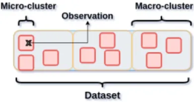
Fig. 1: Distinction between micro and macro clusters

distributional assumptions for the error distributions, since they need not be normal or other parametric distributions. Applying PLS to massive high-dimensional data is problematic because the data processing is computationally ex-pensive. This has limited large-scale applications of PLS in practice. To reduce the computational burden, researchers usually apply a specific model design, such as the Clusterwise PLS [3,21,12].

In this paper, we address a Clusterwise problem where the response variablesyare explained by the explanatory variablesx, organized into clusters. The statistical model which results from simultaneously treating all observations (i.e. a single macro-cluster) may be of low prediction quality. To overcome this problem we use two nested levels of clustering (i.e. macro- and micro- clusters) illustrate in Figure1and compute one model per macro-cluster based on a micro-batch strategy where micro-clusters are shifted from one macro-cluster to another. A standard approach to ob-tain clusters within a regression framework is Clusterwise regression (which is also known as typological regression) [6,18].

Clusterwise regression assumes that there is an underlying clustering structure of the observations and that each cluster can be revealed by the fit of a specific regression model based on micro-clusters. More formally, Clusterwise regression simultaneously looks for a partition of the observations into clusters which minimizes the overall sum of squared error. For Clusterwise methods, a crucial component is to describe the local relationships between the vari-ables measured on the observations within the same cluster. This is handled in this paper by micro-batch approaches. The remainder of the paper is organized in three sections. Section2summarizes previous results which are related with our work. In Section3, the traditional PLS and the micro-batch version are presented. Section 4 focuses on the performance indicators including the prediction quality, execution times and scalability. Section5 contains the conclusions and future perspectives of our work.

Used notations

In the following read, matrix are in bold upper case, vectors in bold lower case. Micro-clusters are those generate after being applied a clustering algorithm , herek-means. Macro-clusters are those generated for the Clusterwise purpose, their number will be equal toG.XandYare respectively the data and response matrix. Response variables will useyandxwill stand for the explanatory variables.

2. Related works

Existing Clusterwise methods seek clusters within a regression framework while simultaneously minimizing the sum of squared error computed over all the clusters. These methods can be viewed as extensions of thek-means cluster-ing from unsupervised learncluster-ing to the regression set-up. As in standard regression, ordinary least squares or maximum likelihood estimation can be used to get the quality of the regression coefficients. Thesek-means like algorithms are

based on a least square error criterion have been proposed by [2,7]. A multivariate regression for heterogeneous data which takes into account both the between- and the within-cluster variability has also been proposed [13].

To detect categorical differences in underlying regression models on the other hand, Spath [18] developed

Clus-terwise Regression (CR) which clusters the data points based on the underlying regression model. Related methods exist within the mixture and latent class framework [6]. Other related methods are the principal component regression (PCR) [4] and partial least square regression (PLS) [19,15] which have also been proposed to deal with multicollinear-ity, small sample size, or large number of variables. Specifically, PLS reduces the explanatory variables to those which are maximally related (in terms of squared covariance) as possible to the objective function.

(4)

Beck Gaël et al. / Procedia Computer Science 144 (2018) 239–250 241

Beck Gaël, Azzag Hanane, Bougeard Stéphanie, Lebbah Mustapha, Niang Ndèye/Procedia Computer Science 00 (2018) 000–000 3 In the framework of component-based path-modeling methods, several Clusterwise methods have been applied in the marketing field (for an early review, refer to [16]). In [9] the authors propose the widely-used finite-mixture PLS (FIMIX-PLS) which assume multivariate normally distributed data. In [10], fuzzy Clusterwise generalized structured component analysis (FCGSCA) is proposed. In [8] the authors propose REBUS-PLS which came from the hierarchical clustering based on a similarity measure defined from the residuals coming from the same models. [17] proposed PLS-IRRS which identifies homogeneous clusters that have similar residual values.

In the field of multigroup analysis where the groups of observations are knowna prioriClusterwise simultaneous component analysis (CW-SCA) seeks clusters among groups of observations rather than among observations [5]. It is worth noting that likelihood-based methods are relevant for data exploration or modeling but are unable to be utilized for prediction as dependent values are needed to compute the likelihood.

3. Micro-Batch PLS for Clusterwise

In this section we present a new mb-CW-PLS algorithm based on combining clustering and PLS. We first review the classical PLS algorithm and then we focus on our proposition.

3.1. Partial Least Square (PLS)

We use the common notation where scalars are defined as italic lower case (x,y), vectors are in bold lower case (x,y) and matrices as bold upper case (X,Y).

PLS regression is a technique that generalizes and combines features from principal component analysis and multi-ple regression. LetX={x₁, . . .xN}beNvector observationsxi=(xi1, . . . ,xip)∈ p, described by the vector response variablesY={y₁, . . . ,yn}whereyi=(yi1, . . . ,yiq)∈ q. Each pair of explanatory and response variables in the model is denoted by the concatenated vectorzi = (xi;yi). The matricesYandXare assumed to be pre-whitened (i.e., the sum of each variable is zero and its norm is one). The superscriptT denotes the matrix transpose operation, e.g.XT andIthe identity matrix.

PLS regression is particularly well-suited when the matrix of explanatory variablesXhas more features pthan observations, and when there is multicollinearity among theXvalues. The goal of PLS regression is to predictY

fromXand to describe their common structure. WhenYis a vector andXis sufficiently regular, this goal could be

accomplished using ordinary multiple regression. PLS solves the problem that arises when number of observations (N) is much lower than the number of variables (p).

PLS regression performs a simultaneous decomposition ofXandY with the constraint that these components capture as much as possible of the covariance betweenXandY. More formally,XandYare decomposed as follows:

X=TPT+E, xik= r j=1 ti jpk j+eik (1) Y=UQT+F, yim = r j=1 ui jqm j+fim (2)

whereTandUare ther-dimensional latent representations ofXandYof size of N×r,PandQare the loading matrices with size ofp×randq×r,EandFare the residual matrices. Thus PLS implements the following optimization problem:

(p,q)=argmax_p₌_q₌₁ cov(T,U)

(5)

Once the decomposition of theXandYis carried out, we can continue with computing the regression coefficients.

The latter are defined as the minimizers of the residual error argmin_BY−XB2

whereBis apbyqregression coefficient matrix. Suppose there is a linear relationship such that

U=TD+H

whereDis anr×rdiagonal matrix, then

Y=TCT+F∗

whereCT ₌_DQT_and_F∗₌_HQT ₊_F_{. Based on the previous expressions, the response matrix is expressed as}

Y=XP(PTP)−1CT+F∗EP(PTP)−1CT.

The PLS regression coefficient is thus

B=P(PTP)−1CT

For the brevity, we have discussed the PLS where the variables form a single macro-cluster. When the data consist of non-homogeneous macro-clusters, it is necessary to decompose the regression according to these macro-clusters, for example, using the Clusterwise techniques described in Section2. These techniques have many bottlenecks as the scalability for a large number of observations and variables. One of the main objectives of this paper is to integrate the micro-batch processing into the Clusterwise PLS to resolve these scalability issues.

3.2. New model: Micro-Batch Clusterwise PLS (mb-CW-PLS) 3.2.1. Overview

Our proposed approach mb-CW-PLS (micro-batch Clusterwise Partial Least Squares) has the following properties: • Nested clustering: we combine the PLS with two levels of clustering (macro- and clustering) and

micro-batch optimization approaches to create a new Clusterwise method that can find the underlying structure of the observations and provide each macro-cluster of observations with its own set of regression coefficients.

• Micro-Batch processing (divide and conquer strategies): rather than move a single observation from a macro-cluster to another to calculate the regression models in a cross validation approach, we move an entire micro-cluster of points, which we call the micro-micro-cluster shift. These micro-micro-clusters are computed using thek-means clustering, wherekis set as the ratio of dataset size to the desired micro-cluster size.

• Scalability: we use a distributed framework based on Apache Spark/Scala to accelerate the initialization process

and to compute the regression models. For each cross validation, we distribute initializations over the slave processes. Each slave selects the optimal initialization and submits it to the master process, which in turns selects the optimal one among all the results received from the slaves. This decreases execution times inversely proportional to the number of slaves.

(6)

Beck Gaël, Azzag Hanane, Bougeard Stéphanie, Lebbah Mustapha, Niang Ndèye/Procedia Computer Science 00 (2018) 000–000 5

• Usability: the Spark/Scala implementation requires the configuration of a small number of hyper parameters,

and can be utilized in a distributed system or even on a stand-alone terminal with minimal effort, which enlarges

the scope of usability of the PLS.

3.2.2. Mathematical details

We assume that the N observations are clustered into K micro-clusters (or buckets), C = _{C₁, . . . ,Ck, . . . ,CK} whereCk={xi, φ(xi)=k}. Denoteφas the assignment function defined as follow :φ:xi ∈ p → {1, . . . ,k, . . . ,K} (eg. euclidean distance). The partitionCof the micro-clusters is carried as an initialization before running the PLS models. This step can be done using clustering approaches such ask-means.

Denote a second partition level P = {P₁, ...,Pg, ...,PG} of the micro-clusters setCinto Gmacro-clusters (and

K G). ThereforeGis the number of regression models that will be considered (PLS1, ...,PLSg, ...,PLSG). The second level assignment functionΦis defined as:Φ:{C₁, . . . ,Ck, . . . ,CK} → {1, . . . ,g, . . . ,G}.

We introduce Micro-Bach Clusterwise PLS methods (mb-CW-PLS) by assuming two phases of clustering: in the first level theNobservations is clustered inKfixed micro-clusters, and in the second level, theKmicro-clusters are grouped intoGmacro-clusters where each macro-cluster has a specific PLS regression model. Therefore the mb-CW-PLS algorithm searches for an optimal partition of the K micro-clusters intoGmacro-clusters as well as the corresponding set of regression coefficient matrices (B₁, ...,BG) that minimize the overall error described in Equation

3: L(P,B)= G g=1 xi∈Pg Yg−XgBg2 = G g=1 Ck∈Pg xi∈Ck yi−xibTg2 (3)

whereXgandYgdenote the data matrices of thegth macro-cluster respectively ofXandY, i.e.

X=               X1=     x11 . . . x1p .. . xN11 . . .xN1p     .. . Xg=     x11 . . . x1p .. . xNg1 . . .xNgp     .. . XG=    x11 . . . x1p v. . . xNG1 . . . xNGp                      φ(x1) Φ(Cφ(x1)) .. . ... φ(xN)Φ(Cφ(xN))     and Y=               Y1 =     y11 . . . y1q .. . yN11. . .yN1q     .. . Yg=     y11 . . . y1q .. . yNg1 . . .yNgy     .. . YG=     y11 . . . y1q .. . yNG1 . . .yNGq                  

The classical Clusterwise PLS does not provide estimators in reasonable time for largeN. Based on the traditional sequential algorithm, each observationxiis assigned to its optimal cluster and the overall error is updated whenever one observation switches cluster. In order to overcome this problem and to ensure that the error decreases monotoni-cally at each iteration of the algorithm, we propose to use a new sequential micro-batch algorithm. Each micro-cluster

Ckis assigned to its optimal macro-clusterPgand the overall error is updated whenever a micro-cluster switches to a different macro-cluster. Therefore the main idea, instead moving a single observationxifrom its original macro-cluster to other macro-clusters, we move the entire micro-clusterCkwhich containsxiand then re-compute the regression

(7)

model. Starting with an initial partition of macro-clustersP(0)₌_{_P(0)

0 , . . . ,P(0)G}, the algorithm constructs iteratively a sequence{P(s)_,_B(s)₎_}_,_s_>_{0, in the following way:}

• For eachg∈ {1. . . ,G},P(0)_{is given by the least square estimators of the PLS regression using the points of the}

macro-clusterPg.

• Given (P(s)_,_B(s)

g ), then for each macro-cluster

Pg∈ {P1, . . . ,PG}, P(s+1) g ={(Xi,Yi) :Yi−XiB(gs1) 2 <Yi−XiB(gs2) 2_,_∀_g 1g2}. (4)

The resultingB(s+1)_{are the PLS estimators using the data partitioned by}_P(s+1)_{. The sequence}_{₍_P(s)_,_B(s)₎_}

s≥0is

such that

L(P(s),B(s)₎_≥_L₍_P(s+1)_,_B(s+1)_), _∀_s_≥₀ and so it is convergent.

• Repeat above step for all micro-clustersCkwhich are re-assigned to their optimal macro-clusterPg. This guar-antees that the overall error decreases monotonically at each change in assignment.

The mb-CW-PLS algorithm finds simultaneously an optimal partition of the fixedKmicro-clusters (buckets) into P={P₁, ...,Pg, ...,PG},Pg={Ck,Φ(Ck)=gand

∀xi∈Ckφ(xi)=k}and the regression models associated to each macro-clusterg. Finally the best cross-validated

try is selected based on the Root Mean Squared Error (RMSE) [20] score. This metric evaluate the prediction accuracy of the fitted regression,

RMS E=

N

i=1( ˆyi−yi)2

N

where ˆyiis the predicted value,yithe true value andNthe number of data points. This method is summarized in the Algorithm1.

3.3. Implementations specificities

In order to get an efficient distributed implementations, we decided to apply the Clusterwise logic through Spark

framework. As explained previously in order to apply a regression in the faster way, data should be inside the machine which perform linked operations. Then rather than to distribute piece of data through nodes in order to avoid shuffling,

we put the entire dataset on each node using thesc.broadcast(dataset)function. Once this step done, we distribute simultaneously every initializations which correspond toCV×INIThomogeneously over nodes. It allows to each node to perform sequentially theirCV×INIT

nodes Clusterwise initializations, via amapPartitionsfunctions where the number of Spark partitions isCV×INIT. TheMappart achieved weaggregateByKeyobtained results where theKeyis a Cross-Validation index. We decided to use the non-parametrick-nearest neighbors method to assign observations to their closest macro-clusterPg in order to apply the associatedPLSg. Finally, based on RMSE scores, the best model is selected over Cross-Validations.

(8)

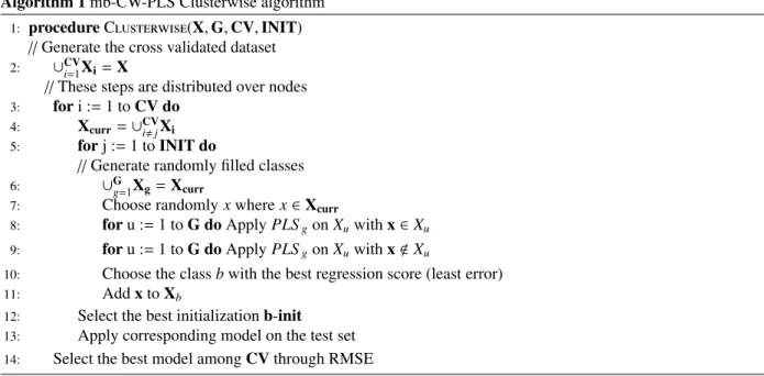
Algorithm 1mb-CW-PLS Clusterwise algorithm 1: procedureClusterwise(X,G,CV,INIT)

//Generate the cross validated dataset

2: _∪CV_i₌₁X_i=X

//These steps are distributed over nodes

3: fori :=1 toCV do

4: X_curr=∪CV_i_jX_i

5: forj :=1 toINIT do

//Generate randomly filled classes

6: _∪G_g₌₁X_g=X_curr

7: Choose randomlyxwherex_∈X_curr

8: foru :=1 toG doApplyPLSgonXuwithx∈Xu 9: foru :=1 toG doApplyPLSgonXuwithxXu

10: Choose the classbwith the best regression score (least error)

11: AddxtoXb

12: Select the best initializationb-init 13: Apply corresponding model on the test set 14: Select the best model amongCVthrough RMSE

Package availability. The mb-CW-PLS method described in this article are implemented in Spark/Scala

and will be available on Clustering4Ever github repository at https: // github. com/ Clustering4Ever/ Clustering4Ever

4. Numerical experiments

4.1. Prediction accuracy vs micro-cluster sizes

In contrast to the regular PLS regression, micro-batch Clusterwise PLS providesGregression models correspond-ing toGmacro-clusters. The iterative cross validation process is as follows: macro clusters are initiated by assigning them randomly each point, for standard Clusterwise, or each micro-clusterCkfor micro-batch Clusterwise. Then the PLS is applied to each macro-cluster, once it is achieved, one observation or one micro-clusterCkis moved inside all other macro-clusterPgin order to compute new PLS regressions. Therefore we run one regression per macro-cluster with and without a specific observation or micro-cluster given 2×Gregressions. Once least squares have been com-pared over all combinations, the point or the micro-clusterCk is assigned to the macro-clusterPg which yields the minimal error. For our experiments different datasets listed in Table1of various sizes have been used. Most of them

came from UCI repository [11].

Dataset n Xsize,p Ysize,q

Yacht Hydrodynamics 308 6 1

Forest Fire 517 10 1

Wine Quality Red 1599 11 1

Wine Quality White 4898 11 1

SimData 400 10 3

Table 1: Overview of data sets.

The evolution of the RMSE in Table3with the value of micro-cluster sizeNkshows that we can efficiently decrease the RMSE with our approach (mb-CW-PLS). We observe a property of Clusterwise methods that increasing number of macro-clustersGreduces the RMSE score. On the other hand, a lowerGallows to use larger values ofNk. In Table3,

(9)

N/A entry indicates that we cannot execute the algorithms under these conditions due to risk of generate empty class

which will falsify quality of results. First we seek for the optimal number of macro-clustersG, then we search for the optimal size of the micro-clusters (buckets)Nk. The first performance criterion is the Root Mean Square Error of prediction as evaluated with a ten-fold cross-validation procedure. Not surprisingly, mb-CW-PLS always improve the Root Mean Square Error (RMSE) of prediction while taking into account the cluster sizeNk.

We observe a property of Clusterwise methods that an increasing number of macro-clustersGreduces the RMSE score. On the other hand, a lowerGallows to use larger values ofNk. In Table3, N/A entry indicates that the choice of

tuning parameters does not lead to a well-defined solution e.g. if we set high value ofNkwe could inconveniently mov-ing every micro-cluster in a macro-cluster to others macro-cluster. However every macro-cluster have to be present in order to compare score of the different generated models. If this happened, then we re-tried with a different

initializa-tion, but a threshold of the number of attempts is fixed before considering tuning parameters ill-posed. The number of clustersKin thek-means clustering isK =N/Nk, the number of cross validation classes isCV =10, the number of initializations isINIT =20 and the number ofknearest neighbors for PLS model assignation is 20. Note that for

Nk=1 is equivalent to the standard CW-PLS.

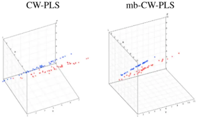
Figure2illustrates results with the three output dimensionsYfrom SimData dataset. We observe that the predicted values (in red) are closer to the true values (in blue) for the mb-CW-PLS than with CW-PLS. The corresponding RMSE is referenced in Table3.

CW-PLS mb-CW-PLS

Fig. 2: Comparison of Clusterwise regression CW-PLS vs mb-CW-PLS for SimData ’sY. True responses are in blue and predicted one are in red

4.2. Comparison to existing regression methods

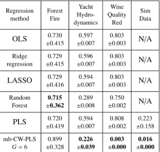
To compare our PLS and mb-CW-PLS regressions to other regression methods, we took the experimental data sets with a single response variable (q = 1). We then fit models for the OLS, Ridge regression, LASSO and Random

Forest using code from theSmile library(https://haifengl.github.io/smile/). 500 replicates of 90% random sampled are taken as training data, then the RMSE based on the remaining 10% test data is computed. The RMSEs are shown in Table2. We observe that PLS provides at least as well the the OLS, Ridge regression and the LASSO, and less well than the Random Forest for the Forest Fire, Yacht Hydrodynamics and Wine Quality Red. The proposed mb-CW-PLS outperforms these methods, in some cases by a substantial margin, in terms of the RMSE. Furthermore, for the SimData which has 3 response variables (q =3), the PLS and mb-CW-PLS are able to produce results, whereas the

other regressions cannot provide results.

4.3. Comparison of prediction accuracy and execution times

Table3shows the RMSE scores and the execution times for CW-PLS and mb-CW-PLS. Let recall that CW-PLS is equivalent to mb-CW-PLS withNk = 1. Figure4aillustrates some of these results indicating that the higher we setG the better can be our results with a smaller standard deviation. This result is partially intuitive in that sense that the more specialized cluster we build, the more effective will be model build on them. The counter part of this

(10)

Regression method Forest Fire Yacht Hydro-dynamics Wine Quality Red Sim Data OLS _±0.730_0.415 _±0.597_0.007 _±0.803_0.003 N/A Ridge regression ±0.7290.415 ±0.5960.007 ±0.8030.003 N/A LASSO _±0.729_0.416 _±0.594_0.007 _±0.803_0.003 N/A Random Forest ±0.7150.362 ±0.2890.008 ±0.7500.002 N/A PLS 0.720 ±0.419 0.594 ±0.007 0.808 ±0.002 0.223 ±0.158 mb-CW-PLS G=6 0.899 ±0.328 ±0.2260.039 ±0.0030.000 ±0.0160.000

Table 2: Comparison of the different regression methods. The first row indicates the mean RMSE followed by the standard deviation. N/A entry

indicates that we cannot execute the algorithms under these conditions

ones. Indeed execution times is much faster as Figure3chighlight it, especially on bigger datasets. The micro-batch processing which produces the micro-clusters allows these decrease in execution time without sacrificing too much of the prediction accuracy as it is exposed on Figure4b-4c. In some case as with the Wine Quality Red dataset we even observe better results. An interesting thing holds in the modest RMSE evolutions over differentNkvalues forNk>1.

4.4. Scalability

4.4.1. Scalability with the respect with the number of nodes

The results obtained in Table3were carried in a local environment (i.e. a stand-alone terminal). We now exam-ine the performance of mb-CW-PLS in a true distributed computing set-up. To execute these experiments, we used Grid5000 [1] infrastructure which is one of the biggest French’s laboratories clusters. We used a set-up with two times 8 core Intel Xeon E5-2630v3 or two times 12 cores AMD Opteron 6164 HE CPUs and 128 Gb RAM per node. Table4

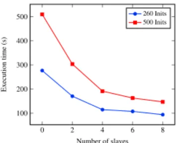
presents average time spend for four run executing a full Clusterwise workflow, which consist to train and test models to select best one. Total initCV×Initcorresponds to the total number of initializations made. Figure3ashows that the execution times decreases efficiently with the number of nodes.

In order to maximize efficiency, we recommend to have 2-3 times more Spark partitions than the total number of

core among every nodes. This approach is not optimal if we have a large data set with few initializations as we do not utilize fully the distributed computational power of Spark. We can also observe that when the number of core nodes is exceeded by the number of initializations, the growth in execution time is almost linear with respect with the number of initializations. As our distributed set-up consists of nodes with 32 cores, a reduction in execution time is observed when the number of initializations is higher than 32.

4.4.2. Scalability with respect with the number of initializations

Figure3bshows the linearity of the problem with the increase of the number of initializations with a set-up of 8 slave nodes. This results illustrate that initializations are well distributed among nodes which allows an efficient

computations of the algorithm.

5. Discussions and conclusion

This work present a new Clusterwise PLS regression algorithm, which brings multiple improvements. First, the micro-batch processing facilitates a drastic reduction in execution times, keeping the same magnitude of prediction accuracy. Second, the distributed implementation enables the test with a large number of initializations in order to

(11)

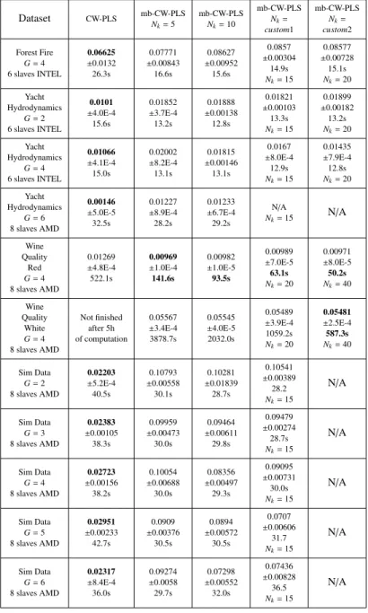
10 Beck Gaël, Azzag Hanane, Bougeard Stéphanie, Lebbah Mustapha, Niang Ndèye/Procedia Computer Science 00 (2018) 000–000 Dataset CW-PLS mb-CW-PLS_N k=5 mb-CW-PLSNk=10 mb-CW-PLS Nk= custom1 mb-CW-PLS Nk= custom2 Forest Fire G=4 6 slaves INTEL 0.06625 ±0.0132 26.3s 0.07771 ±0.00843 16.6s 0.08627 ±0.00952 15.6s 0.0857 ±0.00304 14.9s Nk=15 0.08577 ±0.00728 15.1s Nk=20 Yacht Hydrodynamics G=2 6 slaves INTEL 0.0101 ±4.0E-4 15.6s 0.01852 ±3.7E-4 13.2s 0.01888 ±0.00138 12.8s 0.01821 ±0.00103 13.3s Nk=15 0.01899 ±0.00182 13.2s Nk=20 Yacht Hydrodynamics G=4 6 slaves INTEL 0.01066 ±4.1E-4 15.0s 0.02002 ±8.2E-4 13.1s 0.01815 ±0.00146 13.1s 0.0167 ±8.0E-4 12.9s Nk=15 0.01435 ±7.9E-4 12.8s Nk=20 Yacht Hydrodynamics G=6 8 slaves AMD 0.00146 ±5.0E-5 32.5s 0.01227 ±8.9E-4 28.2s 0.01233 ±6.7E-4 29.2s N/A Nk=15 N/A Wine Quality Red G=4 8 slaves AMD 0.01269 ±4.8E-4 522.1s 0.00969 ±1.0E-4 141.6s 0.00982 ±1.0E-5 93.5s 0.00989 ±7.0E-5 63.1s Nk=20 0.00971 ±8.0E-5 50.2s Nk=40 Wine Quality White G=4 8 slaves AMD Not finished after 5h of computation 0.05567 ±3.4E-4 3878.7s 0.05545 ±4.0E-5 2032.0s 0.05489 ±3.9E-4 1059.2s Nk=20 0.05481 ±2.5E-4 587.3s Nk=40 Sim Data G=2 8 slaves AMD 0.02203 ±5.2E-4 40.5s 0.10793 ±0.00558 30.1s 0.10281 ±0.01839 28.7s 0.10541 ±0.00389 28.2 Nk=15 N/A Sim Data G=3 8 slaves AMD 0.02383 ±0.00105 38.3s 0.09959 ±0.00473 30.0s 0.09464 ±0.00611 29.8s 0.09479 ±0.00274 28.7s Nk=15 N/A Sim Data G=4 8 slaves AMD 0.02723 ±0.00156 38.2s 0.10054 ±0.00688 30.0s 0.08356 ±0.00497 29.3s 0.09095 ±0.00731 30.0s Nk=15 N/A Sim Data G=5 8 slaves AMD 0.02951 ±0.00233 42.7s 0.0909 ±0.00376 30.5s 0.0894 ±0.00572 30.5s 0.0707 ±0.00606 31.7 Nk=15 N/A Sim Data G=6 8 slaves AMD 0.02317 ±8.4E-4 36.0s 0.09274 ±0.0058 29.7s 0.07298 ±0.00552 32.0s 0.07436 ±0.00828 36.5 Nk=15 N/A

Table 3: Comparison of CW-PLS and mb-CW-PLS. The first row is the mean RMSE followed by the standard deviations and the execution times. N/A indicates that we cannot execute the algorithms

# total init local 2 slaves 4 slaves 6 slaves 8 slaves 260 276.6 170.3 114.6 107.4 93.9 500 509.7 303.6 191.2 162.7 146.7

Table 4: Comparison of execution times with different number of initializations and slave processes for the Yacht Hydrodynamics using Intel setup.

find the optimal cross-validated model. One key aspect of the algorithm is the number of regressions needed for one complete run which is 2×G×CV×INIT×N≈1000×Nleading to a quadratic time complexity. Our micro-cluster

(12)

Beck Gaël et al. / Procedia Computer Science 144 (2018) 239–250 249 10 Beck Gaël, Azzag Hanane, Bougeard Stéphanie, Lebbah Mustapha, Niang Ndèye/Procedia Computer Science 00 (2018) 000–000

Dataset CW-PLS mb-CW-PLS_N k=5 mb-CW-PLSNk=10 mb-CW-PLS Nk= custom1 mb-CW-PLS Nk= custom2 Forest Fire G=4 6 slaves INTEL 0.06625 ±0.0132 26.3s 0.07771 ±0.00843 16.6s 0.08627 ±0.00952 15.6s 0.0857 ±0.00304 14.9s Nk=15 0.08577 ±0.00728 15.1s Nk=20 Yacht Hydrodynamics G=2 6 slaves INTEL 0.0101 ±4.0E-4 15.6s 0.01852 ±3.7E-4 13.2s 0.01888 ±0.00138 12.8s 0.01821 ±0.00103 13.3s Nk=15 0.01899 ±0.00182 13.2s Nk=20 Yacht Hydrodynamics G=4 6 slaves INTEL 0.01066 ±4.1E-4 15.0s 0.02002 ±8.2E-4 13.1s 0.01815 ±0.00146 13.1s 0.0167 ±8.0E-4 12.9s Nk=15 0.01435 ±7.9E-4 12.8s Nk=20 Yacht Hydrodynamics G=6 8 slaves AMD 0.00146 ±5.0E-5 32.5s 0.01227 ±8.9E-4 28.2s 0.01233 ±6.7E-4 29.2s N/A Nk=15 N/A Wine Quality Red G=4 8 slaves AMD 0.01269 ±4.8E-4 522.1s 0.00969 ±1.0E-4 141.6s 0.00982 ±1.0E-5 93.5s 0.00989 ±7.0E-5 63.1s Nk=20 0.00971 ±8.0E-5 50.2s Nk=40 Wine Quality White G=4 8 slaves AMD Not finished after 5h of computation 0.05567 ±3.4E-4 3878.7s 0.05545 ±4.0E-5 2032.0s 0.05489 ±3.9E-4 1059.2s Nk=20 0.05481 ±2.5E-4 587.3s Nk=40 Sim Data G=2 8 slaves AMD 0.02203 ±5.2E-4 40.5s 0.10793 ±0.00558 30.1s 0.10281 ±0.01839 28.7s 0.10541 ±0.00389 28.2 Nk=15 N/A Sim Data G=3 8 slaves AMD 0.02383 ±0.00105 38.3s 0.09959 ±0.00473 30.0s 0.09464 ±0.00611 29.8s 0.09479 ±0.00274 28.7s Nk=15 N/A Sim Data G=4 8 slaves AMD 0.02723 ±0.00156 38.2s 0.10054 ±0.00688 30.0s 0.08356 ±0.00497 29.3s 0.09095 ±0.00731 30.0s Nk=15 N/A Sim Data G=5 8 slaves AMD 0.02951 ±0.00233 42.7s 0.0909 ±0.00376 30.5s 0.0894 ±0.00572 30.5s 0.0707 ±0.00606 31.7 Nk=15 N/A Sim Data G=6 8 slaves AMD 0.02317 ±8.4E-4 36.0s 0.09274 ±0.0058 29.7s 0.07298 ±0.00552 32.0s 0.07436 ±0.00828 36.5 Nk=15 N/A

Table 3: Comparison of CW-PLS and mb-CW-PLS. The first row is the mean RMSE followed by the standard deviations and the execution times. N/A indicates that we cannot execute the algorithms

# total init local 2 slaves 4 slaves 6 slaves 8 slaves 260 276.6 170.3 114.6 107.4 93.9 500 509.7 303.6 191.2 162.7 146.7

Table 4: Comparison of execution times with different number of initializations and slave processes for the Yacht Hydrodynamics using Intel setup.

find the optimal cross-validated model. One key aspect of the algorithm is the number of regressions needed for one complete run which is 2×G×CV×INIT×N≈1000×Nleading to a quadratic time complexity. Our micro-cluster

0 2 4 6 8 100 200 300 400 500 Number of slaves Ex ecution time (s) 260 Inits 500 Inits

(a) Evolution of the execution times with respect with the number of slaves. Set-up with Intel CPUs

0 0.2 0.4 0.6 0.8 1 1.2 1.4 ·104 40 60 80 100 Number of initializations Ex ecution time (s)

(b) Evolution of the execution times with respect with the number of initial-izations on Yacht dataset. Set-up with 8 AMD slaves 0 10 20 30 40 0 1,000 2,000 3,000 4,000 Micro-cluster size Ex ecution time (s)

Wine Quality Red Wine Quality White

(c) Evolution of the execution times with respect with of the size of micro-cluster for different datatsets

Fig. 3: Evolution of the execution times

(a) RMSE with standard deviation perG

value (b) RMSE with standard deviation permicro-cluster size (c) RMSE with standard deviation permicro-cluster size

Fig. 4: Root Mean Square Error (RMSE)

approach reduce exclusively the number of regression fromNto N

Nk, but we still compute PLS on the whole dataset preventing better time performance. In our future works we will examine methods to decrease the execution time and also to increase prediction quality. Unfortunately, an inevitable bottleneck is the impossibility to decrease the inner complexity of a regression and Clusterwise strategy is very regression greedy. One solution we desire to investigate will be to reduce to a computable size datasets keeping their inner structure in order to train the Clusterwise model. We have engage this work but due to number of existing sketching methods we need to further testing to find an optimal solution. Another important aspect holds in the affectation of a new observation to its closest macro-cluster which is

solved here by thek-nearest neighbors. However others methods can be tested as for example comparison between the observation with macro-clusters centroid which is faster thank-nearest neighbors but potentially less accurate. As explained previously, an important number of initializations is required to guaranty quality due to their random nature. One option we are thinking about is relaunch an initialization over an achieved one in order to benefit from the Clusterwise process. We can also relaunch this process multiple times until we converge toward an optimal score. The computation overhead could be decrease by reducing the number of random initializations. Another quality result issue is linked to micro-clusters we generate, they came from a basick-means version ,using an euclidean dissimilarity, in order to formed our micro-clusters, others clustering techniques could be used and compared to discover which one fit the best a specific need.

References

[1] Balouek, D., Carpen Amarie, A., Charrier, G., Desprez, F., Jeannot, E., Jeanvoine, E., L`ebre, A., Margery, D., Niclausse, N., Nussbaum, L., Richard, O., P´erez, C., Quesnel, F., Rohr, C., Sarzyniec, L., 2013. Adding virtualization capabilities to the Grid’5000 testbed, in: Ivanov, I.I.,

(13)

van Sinderen, M., Leymann, F., Shan, T. (Eds.), Cloud Computing and Services Science. Springer International Publishing. volume 367 of

Communications in Computer and Information Science, pp. 3–20. doi:10.1007/978-3-319-04519-1\_1.

[2] Bock, H., 1969. The equivalence of two extremal problems and its application to the iterative classification of multivariate data. Mathematisches Forschungsinstitut .

[3] Bougeard, S., Abdi, H., Saporta, G., Niang, N., 2017. Clusterwise analysis for multiblock component methods. Advances in Data Analysis and Classification , 1–29.

[4] Charles, C., 1977. R´egression typologique et reconnaissance des formes. Ph.D. thesis. Universit´e Paris IX.

[5] De Roover, K., Ceulemans, E., Timmerman, M.E., Vansteelandt, K., Stouten, J., Onghena, P., 2012. Clusterwise simultaneous component analysis for analyzing structural differences in multivariate multiblock data. Psychological Methods 17, 100.

[6] DeSarbo, W.S., Cron, W.L., 1988. A maximum likelihood methodology for clusterwise linear regression. Journal of classification 5, 249–282. [7] Diday, E., 1976. Classification et s´election de param`etres sous contraintes. Rapport de recherche IRIA-LABORIA .

[8] Esposito Vinzi, V., Trinchera, L., Squillacciotti, S., Tenenhaus, M., 2008. Rebus-pls: A response-based procedure for detecting unit segments in pls path modelling. Applied Stochastic Models in Business and Industry 24, 439–458.

[9] Hahn, C., Johnson, M.D., Herrmann, A., Huber, F., 2002. Capturing customer heterogeneity using a finite mixture pls approach. Schmalenbach Business Review 54, 243–269.

[10] Hwang, H., Desarbo, W.S., Takane, Y., 2007. Fuzzy clusterwise generalized structured component analysis. Psychometrika 72, 181. [11] Lichman, M., 2013. UCI machine learning repository. URL:http://archive.ics.uci.edu/ml.

[12] Lohm¨oller, J.B., 2013. Latent variable path modeling with partial least squares. Springer Science & Business Media.

[13] Martella, F., Vicari, D., Vichi, M., 2015. Partitioning predictors in multivariate regression models. Statistics and Computing 25, 261–272. [14] Montgomery, D.C., Peck, E.A., Vining, G.G., 2001. Introduction to linear regression analysis. .

[15] Preda, C., Saporta, G., 2005. Clusterwise pls regression on a stochastic process. Computational Statistics & Data Analysis 49, 99–108. [16] Sarstedt, M., 2008. A review of recent approaches for capturing heterogeneity in partial least squares path modelling. Journal of Modelling in

Management 3, 140–161.

[17] Schlittgen, R., Ringle, C.M., Sarstedt, M., Becker, J.M., 2016. Segmentation of pls path models by iterative reweighted regressions. Journal of Business Research 69, 4583–4592.

[18] Sp¨ath, H., 1979. Algorithm 39 clusterwise linear regression. Computing 22, 367–373.

[19] Vinzi, V.E., Lauro, C.N., Amato, S., 2005. Pls typological regression: algorithmic, classification and validation issues, in: New developments in classification and data analysis. Springer, pp. 133–140.

[20] Willmott, C.J., Matsuura, K., 2005. Advantages of the mean absolute error (mae) over the root mean square error (rmse) in assessing average model performance. Climate research 30, 79–82.