Introduction
Multiple sequence alignments (MSAs) are essential instruments for prediction of protein structure and function, phylogenetic inference, and other tasks related to sequence analysis.1 Data in MSAs are usually represented in a matrix form, such that the elements in the same column are homolo-gous, occupy the same place in the genome/protein, and usu-ally have a similar function in the protein structure. Because structure and function may diverge through time as a result of evolutionary processes, making such alignments becomes increasingly difficult when MSAs include sequences sharing a last common ancestor (LCA) very distant in time.2 Sequences in an MSA whose last common ancestor is much more evo-lutionarily distant than that of the remaining sequences in the alignment can be denoted as divergent sequences. This scenario may also arise as a result of horizontal gene transfer processes and also through errors and mistakes during the different phases leading to an MSA. The methods used for aligning sequences try to maximize the number of match-ing residues by usmatch-ing a scormatch-ing scheme that penalizes mis-matches and lack of homologous residues. To this end, gaps are introduced in the alignment. Usually, the more divergent the sequences, the more gaps are introduced to make homolo-gous sequence elements match.3–5
Gaps in an MSA can result from the acquisition or loss of biological information represented by nucleotide or amino acid residues. Occasionally, it is difficult to identify the real cause between these two possibilities, but in any case, in order to maintain the homology in not fully conserved areas, it is necessary to insert gaps. In addition, current methods for constructing MSAs are not perfect and often introduce some errors and noise in the alignments.6,7 These errors become more frequent as more divergent sequences are included in an MSA, and they can seriously affect subsequent analyses.8,9
Filtering the alignments through the removal of posi-tions (columns) of dubious homology is a common practice to increase the phylogenetic signal in the MSA and remove noise.10 Most methods used in phylogenetic inference assume that sites evolve in an independent manner from each other. Thus, removing some columns is expected to enhance the signal-to-noise ratio in the MSA. The columns remaining after filtering are used to construct the phylogeny although evidence rejecting site independence has been published.11 In consequence, several authors have proposed improving MSAs through the elimination of columns correspond-ing to weakly conserved or very divergent regions.10,12,13 Several software tools use this approximation. The popular gBlocks is based on searching for regions with contiguous
Alignments and Detect Outliers
alvaro chiner-oms
1,2and fernando González-candelas
1,21Joint Research Unit “Infection and Public Health” FISABIO, Cavanilles Institute for Biodiversity and Evolutionary Biology, University of Valencia, Paterna, Valencia, Spain. 2CIBER in Epidemiology and Public Health, Madrid, Spain.
AbstrAct: We present EvalMSA, a software tool for evaluating and detecting outliers in multiple sequence alignments (MSAs). This tool allows the identification of divergent sequences in MSAs by scoring the contribution of each row in the alignment to its quality using a sum-of-pair-based method and additional analyses. Our main goal is to provide users with objective data in order to take informed decisions about the relevance and/or pertinence of including/retaining a particular sequence in an MSA. EvalMSA is written in standard Perl and also uses some routines from the statistical language R. Therefore, it is necessary to install the R-base package in order to get full functionality. Binary packages are freely available from http://sourceforge.net/ projects/evalmsa/for Linux and Windows.
Keywords: multiple sequence alignment, gappiness, outlier sequence
CitAtiOn: chiner-oms and González-candelas. Evalmsa: a Program to Evaluate multiple sequence alignments and Detect outliers. Evolutionary Bioinformatics 2016:12 277–284 doi: 10.4137/EBo.s40583.
tYPE: original research
RECEivED: July 18, 2016. RESubMittED: october 02, 2016. ACCEPtED fOR PubliCAtiOn: october 05, 2016.
ACADEMiC EDitOR: liuyang Wang, associate Editor
PEER REviEw: five peer reviewers contributed to the peer review report. reviewers’ reports totaled 1685 words, excluding any confidential comments to the academic editor.
funDing: this study was supported by ministerio de Economía y competitividad, spanish Government (projects Bfu2011-24112 and Bfu2014-58656-r) and Dirección General de salud Pública (Generalitat valenciana, spain). ac-o was a recipient of a formación de Profesorado universitario predoctoral fellowship from ministerio de Educación, spanish Government and was awarded with a grant ayuda de inicio a la Investigación from Universidad de Valencia. The authors confirm that the funders had no
influence over the study design, data collection and analysis, decision to publish, content of the article, or selection of this journal.
COMPEting intEREStS: Authors disclose no potential conflicts of interest.
CORRESPOnDEnCE: [email protected]
COPYRight: © the authors, publisher and licensee libertas academica limited. this is an open-access article distributed under the terms of the creative commons cc-By-nc 3.0 license.
Paper subject to independent expert blind peer review. all editorial decisions made by independent academic editor. upon submission manuscript was subject to anti-plagiarism scanning. Prior to publication all authors have given signed confirmation of agreement to article publication and compliance with all applicable ethical and legal requirements, including the accuracy of author and contributor information, disclosure of competing interests and funding sources, compliance with ethical requirements relating to human and animal study participants, and compliance with any copyright requirements of third parties. this journal is a member of the committee on Publication Ethics (coPE). Published by libertas academica. learn more about this journal.
conserved positions, with a minimum number of gaps and highly conserved flanking positions.12 Other tools, such as T-Coffee, estimate the alignment confidence by a progressive
approach.14 GUIDANCE also calculates a confidence score
that measures the robustness of the guide tree used for con-structing the alignment.15 Despite the popularity of all these tools, some authors indicate that current filtering methods still lead to inaccurate phylogenetic trees and new filtering methods and algorithms are needed.16
More recently, a different approach has been taken. Some-times, a divergent sequence is included in a group of conserved or close (in evolutionary terms) sequences. This inclusion can alter the whole alignment, and in that case, gaps must be intro-duced to maintain homologous and conserved areas. In many cases, gaps are inserted erroneously, and they not only become uninformative but can also decrease the quality of the global alignment.17 The distortion introduced in the alignment affects not only a few columns but also almost the entire MSA. In these situations, and in order to improve the alignment quality, it is necessary to decide whether divergent sequences should be removed from the MSA. A similar question can appear when working with a large number of sequences obtained from public databases, and we must decide which of them should be included in the final analyses. We may accidentally include nonhomologous, wrongly identified, or even reversed sequences. All these situations can lead to an important loss of quality in the data and in a waste of time until we realize of these errors. In these cases, we should identify those divergent sequences as if they were outliers from the rest of the data. Outliers are patterns of data that do not match with the majority of the pat-terns in a dataset. The identification of outliers has been studied in the statistics community for a long time, and it is an impor-tant area in fields such as image processing, fraud detection, and medical anomaly detection.18 Divergent sequences can act as outliers altering the results of posterior analyses and leading to erroneous conclusions.
OD-seq, a recently published tool, also identifies diver-gent sequences in an MSA by finding those cases with an anomalous average distance compared to the remaining sequences.19 OD-seq computes all possible pairwise distances, counting the number of positions with gaps in one sequence and not in the other. Although this is a valid starting point, we consider that more information is needed to make a proper revision of the alignment.
We have developed a software tool to help users in the supervision, comparison, and decision-making tasks after obtaining an MSA. The principal goal of EvalMSA is to pro-vide an objective view of the influence of each sequence on the quality of the MSA. We implement a novel method for detecting the contribution of each individual sequence to the insertion of gaps in the alignment, along with other classic methods such as sum-of-pairs (SP), and provide a statistical evaluation of the improvement in alignment quality if the offending sequences are removed from the MSA.
Methodology
EvalMSA performs different analyses in order to find diver-gent sequences or outliers in an MSA. First, the program ana-lyzes the original length of the sequences used to construct the alignment. Then, EvalMSA calculates the contribution of each sequence to the alignment quality to assess its relative importance in the MSA and assigns a weight to each sequence. Finally, the tool evaluates the contribution of each sequence to introduce gaps in the remaining sequences of the alignment by computing a parameter denoted gappiness. Users can also mark some sequences as reference in case they have been used as outgroups in the alignment. These reference sequences will not be taken into account when summarizing the results and in the identification of those sequences with less weight, more gaps, or higher gappiness value.
Preanalysis. Basic statistics on sequence length can read-ily detect the presence of wrong/misaligned sequences in an MSA, possibly as the result of unnoticed errors at selecting, downloading, or introducing sequence data into the align-ment. In a preliminary analysis, EvalMSA reports some parameters related to the original sequence lengths, such as mean, median, standard deviation, quartiles, and outliers. Typical errors, such as including a single gene into an align-ment of complete genomes, can be identified in this way.
Gappiness value. A truly divergent sequence, evolu-tionarily very distant from the rest, can introduce large gaps in a multiple alignment. Hence, we need to identify those sequences that introduce more gaps in the other sequences. To look for these sequences, we first identify the columns with more gaps than residues in that position. The method is independent of the type of residue (amino acid or nucleotide). For each sequence (row), we count the number of columns having a residue when most of the sequences have a gap. By calculating the number of gaps that each sequence generates in the rest, we can rank them by gap-generation capacity.
To evaluate the capacity of each sequence to introduce gaps in the alignment, a gappiness value (gpp) is calculated. The higher the gpp value of a sequence, the larger the num-ber of gaps it can introduce in the remaining sequences of the alignment. In consequence, as the gpp value increases, the probability that the corresponding sequence is strongly diver-gent from the rest increases as well.
For a given sequence, the gpp value is initialized at 0 and is incremented when a position is found to have a residue and the remaining sequences (over a threshold) have a gap. The value of the increment is inversely proportional to the number of sequences having a residue in that position. A gpp value is calculated for each sequence and, when the evaluation is completed, is compared with the rest. The sequence with the largest gpp value is considered as the sequence that introduces more gaps in the MSA. This value is calculated as follows:
Given an alignment with K sequences and L positions. For each column in the alignment, a Cn value indicating the number of positions that are residues is defined (no gap).
f(s,n) is defined as the number of residue positions with Cn = n, in sequence s. Then: gpps n K CL Kn f s n k =
∑
= ( − )* ( , ) * 1An example of the application of this expression and more details can be found in the Supplementary files.
evaluating the original alignment score and defining the gap penalty. For each alignment, the program calculates a score that will be a quality measure. To calculate this score, we use the SP method. The SP score takes into account all the pairwise information in the alignment and is one of the most popular, simple methods used for scoring an MSA. Using a scoring matrix in conjunction with the SP method allows us to score each sequence based on its similarity and mismatches with the rest of the sequences. A more detailed explanation about how the SP method is implemented in EvalMSA is pro-vided in the Supplementary files.
This system can be used for assessing amino acid or nucleotide alignments through an appropriate scoring matrix. Scoring matrices typically do not include gap penalty values. One of the main problems with the SP method is the assess-ment of gap penalties. During the alignassess-ment process, inserting a gap in a sequence is always penalized. This penalty depends on how evolutionarily close the sequences are and on whether it corresponds to a gap opening or a gap extension. In our case, we will penalize all the gaps with the same value, but this can be changed easily.
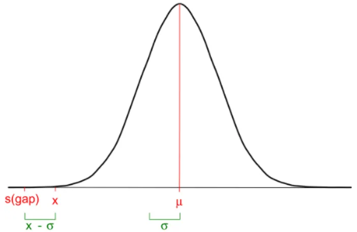
Sometimes, the alignment process generates large gaps due to errors or the use of inappropriate or very divergent sequences. These often lead to a serious decrease in the quality of the align-ment. We assume that, during the evolutionary process, losing or gaining a residue is less likely than the substitution of an amino acid or nucleotide by another. A gap in just one sequence means lack of homology (due to insertions or deletions) to the rest of the sequences and represents a loss of information for subsequent analyses. We account for mismatches and for gaps when scoring sequences, but we want to maximize the gap effect and, in consequence, we penalize more those sequences with more gaps. Hence, in our analysis, a gap will be penalized more than a mismatch and gap penalties receive a lower value in the scoring matrix than perfect matches or mismatches. For any set of values defined in the scoring matrix, we approximately obtain a normal distribution (Fig. 1). The gap penalty is defined as:
s gap x( )= −σ
where σ is the standard deviation and x is the lowest value in the matrix.
If the alignment contains symbols that are not defined in the scoring matrix, such as *, ?, and X, they will be assigned the s(gap) value.
evaluating the weight of each sequence on the alignment quality. For each sequence in the MSA, we evalu-ate its weight (or influence) on the alignment quality. For this, each sequence is scored with a method derived from SP.
Given N sequences of length L, aligned forming an MSA matrix M = N × L and a scoring matrix, which provides a score s(x, y) for the alignment of characters x and y, then the score for
ith position in sequence s, w(si), in the matrix is calculated as
w si s m mis
ij j j s N
( )=
∑
=1, ≠ ( , )where mis is the element from sequence s in position i and m ij is the element from sequence j in position i. The global score for sequence s, W(s), results from adding the w score for each position in the sequence:
W s( )=
∑
iL=1w s( )iThe W(s) score can be interpreted as a measure of the
influence of sequence s on the MSA quality.
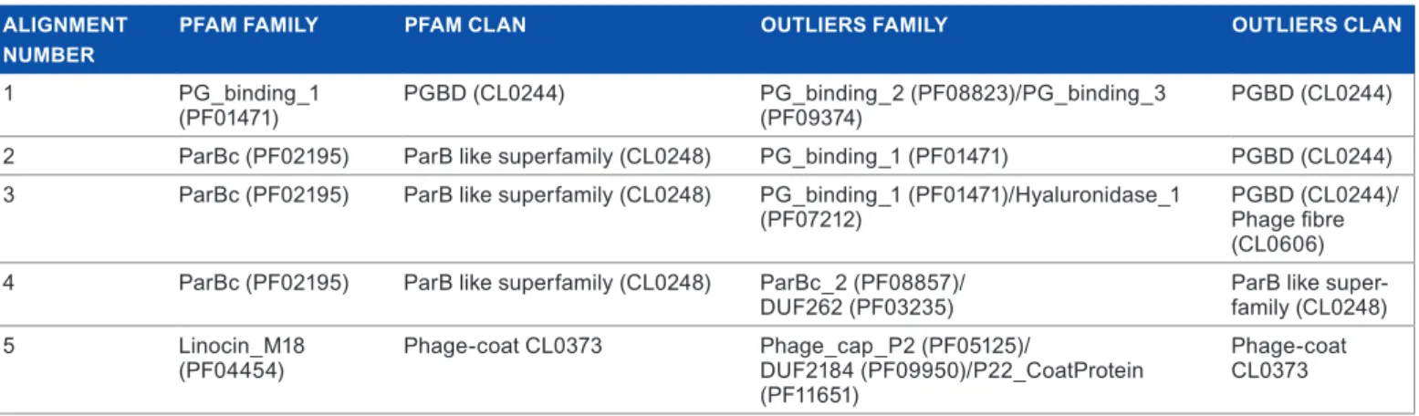
benchmarking. In order to test the accuracy and effi-ciency of the program, we benchmarked our application with alignments from the Pfam database (version 29.0).20 We took seed alignments from peptidoglycan-binding domain (PGBD), ParB, and phage-coat clans and added artificial outliers from Pfam families from either the same or different clans (Table 1). Once the outliers were added, we realigned the sequences using MUSCLE and ClustalW as implemented in MEGA software21 and also using the Expresso algorithm.22 To test if the program works with other types of data rather than with amino acid alignments, we downloaded the mito-chondrial genome sequences of 13 primates from GenBank. We added to this dataset the mitochondrial genome sequence of a reptile (Crocodylus porosus) and made an alignment using the MUSCLE algorithm. The resulting alignments were used as inputs for our program.
s(gap)
x σ σ
x µ
-figure 1. Gap penalty value. using all the values contained in the scoring matrix, we obtained the distribution represented above. a value lower than the rest in the scoring matrix is valued as a gap penalty.
Implementation. The application was implemented in Perl, with some modules imported from BioPerl.23 The results are plotted with the R language, so it is necessary to install the R-base code in order to obtain full functionality of EvalMSA. Complete information about the algorithms and methods used to calculate the numerical values reported by EvalMSA can be found in the Supplementary files. We also provide the alignments used in the benchmarking as an example of use as well as the results of the analyses in the Supplementary files.
results and discussion
We benchmarked our application with six different alignments. Table 1 summarizes the different MSAs used to benchmark the program derived from the Pfam database. To describe the
output of the program in detail, we will explore the results for alignment 5 in Table 1. To construct it, we took the seed align-ment of the Pfam protein family Linocin M18 (PF04454). Then, we added three protein sequences from families belong-ing to the same Pfam clan (CL0373) to the seed alignment and we realigned it. We run EvalMSA with both alignments and compared the results. The program was run with default parameters in all the cases (default gap penalty, default gap threshold, the substitution matrix blosum62 for amino acid alignments, and DNA2 for the nucleotide one).
The returned results can be easily interpreted. Figure 2A (left) shows an example of the preanalysis output, in which a usual sequence length distribution is shown. All the sequences have a similar length (only 30 bp of difference between the
table 1. msas used to benchmark the program. AlignMEnt
nuMbER PfAM fAMilY PfAM ClAn OutliERS fAMilY OutliERS ClAn
1 PG_binding_1
(Pf01471) PGBD (cl0244) PG_binding_2 (Pf08823)/PG_binding_3 (Pf09374) PGBD (cl0244) 2 ParBc (Pf02195) ParB like superfamily (cl0248) PG_binding_1 (Pf01471) PGBD (cl0244) 3 ParBc (Pf02195) ParB like superfamily (cl0248) PG_binding_1 (Pf01471)/Hyaluronidase_1
(Pf07212) PGBD (cl0244)/Phage fibre (cl0606) 4 ParBc (Pf02195) ParB like superfamily (cl0248) ParBc_2 (Pf08857)/
Duf262 (Pf03235) ParB like super-family (cl0248)
5 linocin_m18
(Pf04454) Phage-coat cl0373 Phage_cap_P2 (Pf05125)/Duf2184 (Pf09950)/P22_coatProtein (Pf11651) Phage-coat cl0373 Original alignment Pre-analysis boxplot 265 260 255 Sequence length 250 245 240 235 A
Alignment with outliers Original alignment Alignment with outliers
Pre-analysis boxplot 400 350 Sequence length 300 250 Weight histogram 20 15 10 Number of sequences 5 0 1 0 2 Weight 2 20 17 −15000 −10000 −5000 0 5000 10000 15000 B Weight histogram 15 10 Number of sequence s 5 0 2 2 0 Weight 17 13 11 −55000 −50000 −45000 −40000 −35000 −30000 −25000
Normalized weight plot
1.0 0.8 0.6 Normalized weight (w ) 0.4 0.2 0.0 Sequence index 0 10 20 30 40
C Normalized weight plot
1.0 0.8 0.6 Normalized weight (w ) 0.4 0.2 0.0 Sequence index 0 10 20 30 40 Gappiness plot 0.05 0.04 Gapiness value 0.03 0.02 0.01 Sequence index 0 10 20 30 40 D Gappiness plot 0.35 0.30 0.25 NGapiness value 0.20 0.15 0.10 0.05 0.00 Sequence index 0 10 20 30 40
figure 2. Default output. (A) Preanalysis boxplot showing the original sequence length distribution. (b) Weight score histogram, highlighting the sequences with the highest number of gaps (green line) and with the largest gappiness value (magenta line). (C) normalized weight score distribution. sequence index refers to the list of sequences listed by weight. (D) Gappiness values. sequence index refers to the list of sequences listed by gpp value.
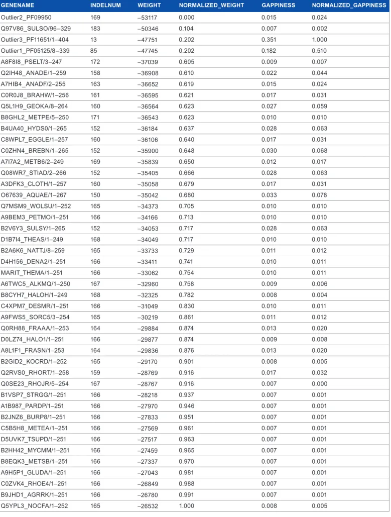
table 2. summary of the results obtained after running the program with dataset 5 aligned with musclE (see table 1).
gEnEnAME inDElnuM wEight nORMAlizED_wEight gAPPinESS nORMAlizED_gAPPinESS
outlier2_Pf09950 169 −53117 0.000 0.015 0.024 Q97v86_sulso/96–329 183 −50346 0.104 0.007 0.002 outlier3_Pf11651/1–404 13 −47751 0.202 0.351 1.000 outlier1_Pf05125/8–339 85 −47745 0.202 0.182 0.510 a8f8i8_PsElt/3–247 172 −37039 0.605 0.009 0.007 Q2iH48_anaDE/1–259 158 −36908 0.610 0.022 0.044 a7HiB4_anaDf/2–255 163 −36652 0.619 0.015 0.024 c0r0J8_BraHW/1–256 161 −36595 0.621 0.017 0.031 Q5l1H9_GEoKa/8–264 160 −36564 0.623 0.027 0.059 B8GHl2_mEtPE/5–250 171 −36543 0.623 0.010 0.010 B4ua40_HyDs0/1–265 152 −36184 0.637 0.028 0.063 c8WPl7_EGGlE/1–257 160 −36106 0.640 0.017 0.031 c0ZHn4_BrEBn/1–265 152 −35900 0.648 0.030 0.068 a7i7a2_mEtB6/2–249 169 −35839 0.650 0.012 0.017 Q08Wr7_stiaD/2–266 152 −35405 0.666 0.028 0.063 a3DfK3_clotH/1–257 160 −35058 0.679 0.017 0.031 o67639_aQuaE/1–267 150 −35042 0.680 0.033 0.078 Q7msm9_Wolsu/1–252 165 −34373 0.705 0.010 0.010 a9BEm3_PEtmo/1–251 166 −34166 0.713 0.010 0.010 B2v6y3_sulsy/1–265 152 −34053 0.717 0.028 0.063 D1B7i4_tHEas/1–249 168 −34049 0.717 0.010 0.010 B2a6K6_nattJ/8–259 165 −33733 0.729 0.011 0.012 D4H156_DEna2/1–251 166 −33411 0.741 0.010 0.011 marit_tHEma/1–251 166 −33062 0.754 0.010 0.011 a6tWc5_alKmQ/1–250 167 −32960 0.758 0.009 0.006 B8cyH7_HaloH/1–249 168 −32325 0.782 0.008 0.004 c4XPm7_DEsmr/1–251 166 −31049 0.830 0.010 0.011 a9fWs5_sorc5/3–254 165 −30219 0.861 0.011 0.012 Q0rH88_fraaa/1–253 164 −29884 0.874 0.013 0.020 D0lZ74_Halo1/1–251 166 −29877 0.874 0.009 0.008 a8l1f1_frasn/1–253 164 −29836 0.876 0.013 0.020 B2GiD2_KocrD/1–252 165 −29170 0.901 0.008 0.005 Q2rvs0_rHort/1–258 159 −28769 0.916 0.017 0.032 Q0sE23_rHoJr/5–254 167 −28767 0.916 0.007 0.000 B1vsP7_strGG/1–251 166 −28218 0.937 0.007 0.001 a1B987_ParDP/1–251 166 −27970 0.946 0.007 0.001 B2JnZ6_BurP8/1–251 166 −27833 0.951 0.007 0.001 c5B5H8_mEtEa/1–251 166 −27569 0.961 0.007 0.001 D5uvK7_tsuPD/1–251 166 −27517 0.963 0.007 0.001 B2HH42_mycmm/1–251 166 −27459 0.965 0.007 0.001 B8EQK3_mEtsB/1–251 166 −27337 0.970 0.007 0.001 a9H5P1_GluDa/1–251 166 −27043 0.981 0.007 0.001 c0ZvK4_rHoE4/1–251 166 −26849 0.988 0.007 0.001 B9JHD1_aGrrK/1–251 166 −26780 0.991 0.007 0.001 Q5yPl3_nocfa/1–252 165 −26532 1.000 0.008 0.005
shortest and the longest sequences). In the right part of Figure 2A, it is possible to identify a pair of sequences that radically differ from the others in terms of sequence length. The weight distribution, as shown in Figure 2B, is also an intuitive way of evaluating the contribution of each sequence to the alignment quality. The left histogram shows that most sequences have a similar weight. The magenta line identifies the sequence with the highest gappiness value, and the green line identifies the sequence with the largest number of gaps. This sequence contributes markedly less than the rest to the alignment quality. The weight of the sequence identified as introducing more gaps (magenta line) does not differ much from the rest of the sequences. On the other hand, the right histogram shows that four sequences had less weight values than the rest. The sequences marked as having more gaps and the one provoking more gaps are in the left part of the histo-gram. The same information is represented in Figure 2C but after normalizing the weight scores and sorting them. In this way, it is easier to appreciate the differences among weighting scores. In the left plot, most of the sequences have a high score and only one of them has a low weight. In the right plot, we can see that at least four sequences have a weight value lower than the rest. Three of these sequences correspond to the artificial outliers that we added to obtain the MSA. Finally, the distri-butions of gappiness values are shown in Figure 2D. Again, by comparing the right and the left plots, we can observe that two of the outliers have higher gappiness values than the rest.
The plots shown in Figure 2 correspond to the standard output of the tool. The program also writes a Comma Separated Values (CSV) file with all the values calculated associated with the sequence names, so additional analyses can be made by the user. Table 2 shows the CSV file obtained from the above exam-ple, in which we can see that the sequence with less weight value corresponds to outlier 2, while the two sequences with the high-est gappiness values are outliers 3 and 1. These results mean that outliers 3 and 1 are the sequences that introduce more gaps in the rest of the sequences. So, probably, their presence is altering the whole alignment. The user can identify them easily as pos-sible outliers. On the other hand, the gappiness value for outlier 2 is really low, so it does not introduce many gaps in the rest of sequences. However, the weight of this sequence is the lowest one so the number of gaps and mismatches is higher than for the rest of the sequences. Hence, outlier 2 sequence should also be taken into account by the user as a possible outlier. In addi-tion to these files, a plain-text file with a short summary of the divergent sequences identified is created.
We have not observed remarkable differences between alignments obtained with different algorithms, such as those implemented in MUSCLE and ClustalW. The outliers were identified correctly in both cases. Moreover, we used the Expresso algorithm21 to construct alignments taking struc-tural information into account. Again, no remarkable dif-ferences were found in the results. So, our program works independently from the algorithm used to align the data.
In addition, we have checked that our program correctly identifies outliers from other data sources such as GenBank sequences. In Supplementary file 2, we have included an alignment of 13 mitochondrial genomes from primates and one mitochondrial genome from a reptile. EvalMSA correctly identifies the reptile sequence as the one with the least weight as well as the highest gappiness value.
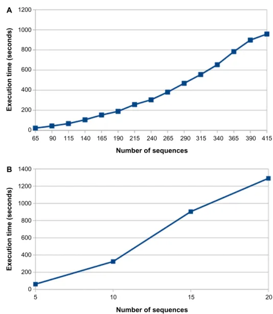
Figure 3 presents the results of a benchmark test show-ing the execution time of the program when run in a personal computer (Intel Core i7–4770 CPU 3.40 GHz, 16 GB RAM, 1 TB HDD) for different MSAs. We tested the program with an MSA of 415 virus and 20 bacterial genomes. The execu-tion time is fast with short (virus) genomes, but it slows down as the number of sequences in the MSA increases. The most time-consuming part of the program is the weight computa-tion. It relies on a nested loop that goes over all the positions for each sequence. So, the time complexity for the program is O(n2). The program is highly recommended for working with viral and bacterial genomes as well as gene alignments.
By default, EvalMSA calculates a gap penalty that depends on the substitution matrix used to score the align-ment. This value, as well as the substitution matrix and the gap threshold used to calculate the gpp value (as detailed in the Supplementary file), can be defined by the user. Also, by default the program provides the BLOSUM62 and PAM70 substitution matrices and a DNA matrix penalizing transitions vs transversions. Users can also define their own matrices to score the alignments according to their needs. In addition, the program accepts command-line arguments so it is easy to include it in a pipeline.
Although a similar tool was recently published,18 the software presented here provides a wider perspective on sequence divergence and can be used complementarily to OD-seq. Similarly to OD-seq, EvalMSA also penalizes gap occurrence, but it takes into account mismatches, gpp values, and the original sequence lengths and gives a graphical and more complete report of the results, thus facilitating a deeper analysis. OD-seq produces results faster, but if the user needs a more detailed analysis, EvalMSA returns more results and accounts for more diverse reasons for sequence divergence.
To compare both programs, we analyzed alignment 5 in Table 1 with OD-seq. This program only identified as outli-ers the introduced sequences 1 and 3 and maintained outlier 2 in the core alignment. The identification of outliers by OD-seq is based on the number of gaps between OD-sequences, but EvalMSA also penalizes mismatches and takes into account gappiness values. Hence, our program can identify the dif-ferent outliers and the cause of their divergence from the rest of the sequences ( gpp value, weight, or number of gaps). In summary, OD-seq can be used as an initial, fast approxi-mation, and EvalMSA can be used as a posterior tool for a deeper analysis.
Evaluating alignments is not a trivial or obsolete prob-lem. The decision of including or not a sequence in a multiple
alignment and subsequent analyses is ultimately made by the investigators. It is important to have a method that allows them to evaluate MSAs with a unique methodology and criterion, so that decisions are based on objective data. Our software tool serves as an objective data provider so that investigators can make decisions based on an objective, easily reproducible method besides their own experience and criterion. Finally, EvalMSA was programmed using Perl and R, so it is portable to almost any platform.
Acknowledgment
We thank Dr Garcia-Garcerá for his help and comments in testing EvalMSA during its development.
Author contributions
Conceived and designed the experiments: FG-C, AC-O. Analyzed the data: AC-O. Wrote the first draft of the article: AC-O. Contributed to the writing of the article: FG-C, AC-O. Agreed the article results and conclusions: FG-C,
AC-O. Jointly developed the structure and arguments for the article: FG-C, AC-O. Made critical revisions and approved the final version: FG-C, AC-O. Both authors reviewed and approved the final article.
supplementary Material
supplementary File 1. Document file with additional details on the methods used in EvalMSA.
supplementary File 2. Alignment files with and without outliers used to benchmark the program.
reFerences
1. Edgar RC, Batzoglou S. Multiple sequence alignment. Curr Opin Struct Biol. 2006;16:368–73.
2. Liu K, Linder CR, Warnow T. Multiple sequence alignment: a major challenge to large-scale phylogenetics. PLoS Curr. 2010;2:1198.
3. Mount DW. Using gaps and gap penalties to optimize pairwise sequence align-ments. CSH Protoc. 2008;2008:db.to40.
4. Kondrashov AS, Rogozin IB. Context of deletions and insertions in human cod-ing sequences. Hum Mutat. 2004;23:177–85.
A 1200 1000 800
Execution time (seconds)
600 400 200 0 65 90 115 140 165 190 215 240 265 290 315 340 365 390 415 Number of sequences B 1400 1200 1000
Execution time (seconds)
800 600 400 200 0 5 10 15 20 Number of sequences
figure 3. Execution time of the program with different alignment sizes. (A) Execution times for msa with different numbers of sequences (sequence length 10 kbp, viral genome). (b) Execution times for msa with different numbers of sequences (sequence length 4.4 mbp, bacterial genomes).
5. Ogurtsov AY, Sunyaev S, Kondrashov AS. Indel-based evolutionary distance and mouse-human divergence. Genome Res. 2004;14:1610–16.
6. Landan G, Graur D. Characterization of pairwise and multiple sequence align-ment errors. Gene. 2009;441:141–47.
7. Landan G. Multiple Sequence Alignment Errors and Phylogenetic Reconstruction. Tel-Aviv: Tel-Aviv University; 2005.
8. Kumar S, Filipski A. Multiple sequence alignment: in pursuit of homologous DNA positions. Genome Res. 2007;17:127–35.
9. Ogden TH, Rosenberg MS. Multiple sequence alignment accuracy and phyloge-netic inference. Syst Biol. 2006;55:314–28.
10. Talavera G, Castresana J. Improvement of phylogenies after removing divergent and ambiguously aligned blocks from protein sequence alignments. Syst Biol. 2007;56:564–77.
11. Nasrallah CA, Mathews DH, Huelsenbeck JP. Quantifying the impact of depen-dent evolution among sites in phylogenetic inference. Syst Biol. 2011;60:60–73. 12. Castresana J. Selection of conserved blocks from multiple alignments for their
use in phylogenetic analysis. Mol Biol Evol. 2000;17:540–52.
13. Capella-Gutierrez S, Silla-Martinez JM, Gabaldon T. trimAl: a tool for auto-mated alignment trimming in large-scale phylogenetic analyses. Bioinformatics. 2009;25:1972–73.
14. Wallace IM, O’Sullivan O, Higgins DG, Notredame C. M-Coffee: combining multi-ple sequence alignment methods with T-Coffee. Nucl Acids Res. 2006;34:1692–99.
15. Penn O, Privman E, Landan G, Graur D, Pupko T. An alignment confidence score capturing robustness to guide tree uncertainty. Mol Biol Evol. 2010;27:1759–67. 16. Tan G, Muffato M, Ledergerber C, et al. Current methods for automated
filter-ing of multiple sequence alignments frequently worsen sfilter-ingle-gene phylogenetic inference. Syst Biol. 2015;64:778–91.
17. Capella-Gutiérrez S, Gabaldón T. Measuring guide-tree dependency of inferred gaps in progressive aligners. Bioinformatics. 2013;29:1011–17.
18. Chandola V, Banerjee A, Kumar V. Anomaly detection: a survey. ACM Comput Surv. 2009;41(3):Article15.
19. Jehl P, Sievers F, Higgins DG. OD-seq: outlier detection in multiple sequence alignments. BMC Bioinformatics. 2015;16:1–11.
20. Finn RD, Bateman A, Clements J, et al. Pfam: the protein families database.
Nucleic Acids Res. 2014;42:D222–30.
21. Tamura K, Stecher G, Peterson D, Filipski A, Kumar S. MEGA6: molecular evolutionary genetics analysis version 6.0. Mol Biol Evol. 2013;30:2725–9. 22. Armougom F, Moretti S, Poirot O, et al. Expresso: automatic incorporation of
structural information in multiple sequence alignments using 3D-Coffee. Nucleic Acids Res. 2006;34:W604–08.
23. Stajich JE, Block D, Boulez K, et al. The Bioperl Toolkit: Perl modules for the life sciences. Genome Res. 2002;12:1611–8.