SERIE DOCUMENTOS DE TRABAJO
No. 65 Junio 2009
STATISTICAL INFERENCE FOR TESTING GINI COEFFICIENTS:
AN APPLICATION FOR COLOMBIA
Luis Fernando Gamboa
Andrés García
Statistical inference for testing Gini coe¢ cients:
An application for Colombia
Luis Fernando Gamboa
yFacultad de Economía
Universidad del Rosario
Bogotá, Colombia
Andrés García
zFacultad de Economía
Universidad del Rosario
Bogotá, Colombia
Jesús Otero
xFacultad de Economía
Universidad del Rosario
Bogotá, Colombia
June 2009
Abstract
This paper uses Colombian household survey data collected over the pe-riod 1984-2005 to estimate Gini coe¢ cients along with their corresponding standard errors. We …nd a statistically signi…cant increase in wage income inequality following the adoption of the liberalisation measures of the early 1990s, and mixed evidence during the recovery years that followed the eco-nomic recession of the late 1990s. We also …nd that in several cases the observed di¤erences in the Gini coe¢ cients across cities have not been statis-tically signi…cant.
JEL Classi…cation: C12; D31; I32.
Keywords: Inequality, Gini coe¢ cient, bootstrap, Colombia.
We would like to thank Russell Davidson, Luis Eduardo Fajardo, Ana Maria Iregui and Jeremy Smith for useful comments and suggestions. The usual disclaimer applies.
yE-mail: [email protected] zE-mail: [email protected]
1
Introduction
Measuring the evolution of income distributions over time and/or across regions, and assessing the e¤ect of policy measures on income concentration are topics of research that have historically received a great deal of attention. To address these topics, authors typically provide comparisons based on the ranking of estimated Gini coe¢ cients, without acknowledging the fact that, being a sample statistic, these co-e¢ cients have associated sampling distributions. For example, Baer and Maloney (1997) review the impact on income distribution of the market-oriented policy re-forms instituted in Latin America during the 1980s. They observe that in the case of Chile, the Gini coe¢ cient fell from 0.49 to 0.47 under the socialist experiment of the Allende government, and then increased to 0.52 during the military dictatorship regime. Then, during 1990-1993, a period of transition back to democracy, the Gini coe¢ cient was 0.51. On the other hand, a comparison of the variation in the Gini coe¢ cient in Mexico during 1986-1992, a period of economic adjustments and lib-eralisation measures, re‡ects an increase from 0.43 to 0.48. As another illustration, Cunningham and Jacobsen (2008) use household survey data from Bolivia, Brazil, Guatemala and Guyana, to construct earnings inequality measures by gender and by racial/ethnic origin. They …nd that for Bolivia the Gini coe¢ cients for white and non-white men (women) are 0.51 (0.54) and 0.53 (0.60), respectively. The question that arises is whether these observed di¤erences in Gini coe¢ cients are statistically signi…cant.
During the last decade or so, a number of authors have considered di¤erent methodologies to estimate the standard error of the Gini coe¢ cient; see Zheng and Cushing (2001), Giles (2004, 2006), Ogwang (2000, 2004, 2006) and Modarres and Gastwirth (2006). However, in a recent paper Davidson (2009) points out that the estimators available in the literature are either mathematically complex to calculate or quite unreliable. For example, Davidson (2009) shows that the jackknife estimator of the variance is not a consistent estimator of the asymptotic variance of the Gini coe¢ cient, and therefore does not give reliable inference. Davidson (2009)
presents a procedure to compute an asymptotically correct standard error for the Gini coe¢ cient based on a relatively simple expression. The work by Davidson has at least three main contributions. First, it provides a bias-corrected estimator of the Gini coe¢ cient. Second, it derives an approximation for the standard error of the Gini coe¢ cient in which it is expressed as a sum of independent and identically distributed (iid)random variables. Third, it illustrates how bootstrap methods can be used to yield reliable inference about the Gini coe¢ cient.
This paper uses Colombian household survey data over the period 1984-2005 to estimate the Gini coe¢ cient for the main seven urban areas, as well as for the country as a whole. Rankings of Gini coe¢ cients based on income distributions for Colombia have been undertaken by Berry and Urrutia (1976), Vélez (1995), Ocampo, Sánchez and Tovar (2000) and Birchenall (2001, 2007), among others. In sharp contrast to this literature, in this paper we estimate standard errors on these Gini coe¢ cients enabling us to test for statistical variation across urban areas and over time. The chosen sample period is interesting because the Colombian government instituted a series of major liberalising reforms in the early 1990s, although this was followed by the deepest recession experienced by the country in the last century, and the subsequent years of recovery.
The paper is organised as follows. Section 2 brie‡y describes the methodology used for the estimation of the Gini coe¢ cient and its corresponding standard error. Section 3 describes the data set used in the paper and summarises the main results. Section 4 o¤ers concluding remarks.
2
Methodology
The standard approach to measuring income inequality is the Gini coe¢ cient, which provides an absolute measure of the extent of inequality. The Gini coe¢ cient ranges from 0, when all individuals have exactly the same income, to 1, when only one
individual has the totality of income and everyone else has nothing at all.1 The Gini
coe¢ cient based on a sample of data is an estimator of the true parameter with an associated standard error.
The Gini coe¢ cient is de…ned as twice the area between the equidistribution line (i.e. the 45o-line) and the Lorenz (1905) curve. Recently Davidson (2009) expressed
the Gini coe¢ cient as:
^ G= 2 bn2 n X i=1 y(i) i 1 2 1; (1)
wherey(i),i= 1;2; ::; n, is the series of order statistics of the income variabley(that
is, the original series sorted in increasing order), and b is the estimated mean of y. Davidson (2009) …nds an approximate expression for the bias of G^, from which he subsequently derives the following bias-corrected estimator of the Gini coe¢ cient, denoted G~, which is given by:
~
G= n
(n 1)
^
G: (2)
While the estimator (2) is still biased, its bias is of order smaller than n 1.
Equation (2) can be used to obtain an estimate of the standard error of G~. Using:
~
Zi = ( ~G+ 1)y(i)+ 2(wi vi); (3)
where wi = (2i 1)y(i)=(2n) and vi = n 1Pij=1y(j), the standard error of the
bias-corrected Gini coe¢ cient is denoted as:
SE G~ = v u u t 1 (nb)2 n X i=1 ( ~Zi Z)2: (4)
Davidson (2009) shows, via simulation experiments, that the asymptotic distri-bution of the Gini coe¢ cient is reliable even for sample sizes of around 100 obser-vations. However, in case the underlying income distribution follows a lognormal
1This range of variation also applies to other inequality measures such as the indices of Atkinson
distribution with a large variance, or when the distribution has heavy tails, reli-able inference can be obtained by applying the bootstrap method. In particular, Davidson (2009) suggests implementing the bootstrap method as follows. First, let
( ~G G0)
SE G~
; (5)
be the test statistic required to test the null hypothesis that the bias-corrected Gini coe¢ cient is equal to G0. Then, one generates b = 1; :::; B bootstrap samples
of size n by resampling with replacement from the observed income data (which is also of size n). For bootstrap sample b;one computes a bootstrap statistic b as in (5), but with G0 replaced by G~, that is the value of the statistic computed
from the observed sample. This is required so that the hypothesis tested should be true of the bootstrap data-generating process. To calculate an interval at nominal con…dence level(1 ), one estimates the =2and1 =2quantiles of the empirical distribution of the bootstrap statistics b.
3
Data and main results
To study the distribution of income in Colombia, we use data from the nationwide household surveys periodically undertaken by the Departamento Administrativo Na-cional de Estadística (DANE). Our period of analysis, which runs from 1984 to 2005, is characterised by the implementation of two di¤erent surveys, namely the Encuesta Nacional de Hogares – ENH (National Household Survey) and the Encuesta Con-tinua de Hogares – ECH (Continuous Household Survey). The former was applied quarterly from 1979 to 2000, and up to 1983 included the four main cities: Bo-gotá, Medellín, Cali and Barranquilla. In 1984 three more cities were added to the ENH: Bucaramanga, Manizales and Pasto. In 2001, the ENH was superseded by the ECH, which is a monthly survey of 13 cities: the original 7 plus Ibagué, Montería, Cartagena, Pereira, Villavicencio and Cúcuta.2
2The ECH also introduced changes in the phrasing of questions aimed at measuring labour
The dataset used in the analysis consists of the hourly wage per worker (in constant prices of 2005) during the period 1984-2005, which is used as a proxy for wage income. The data for each year in the period 1984-2005 was obtained by aggregating the surveys of that year. We use the seven main cities which are available throughout the sample period: Bogotá (Bog), Medellín (Med), Cali (Cal), Barranquilla (Bar), Bucaramanga (Buc), Manizales (Man) and Pasto (Pas), which account for more than seventy percent of the country’s total urban population.
For the purposes of our estimations, individuals who do not report either wage income or having worked during the previous week are excluded from the analysis.3
The evolution of the average hourly wage rate during the sample period, both for each city and for the country, is presented in Table 1.4 The total number of obser-vations ranges from 41,008 in 2003 to 76,946 in 1984. In turn, the median hourly wage in the seven cities varies between $1,596 in 1992 and $2,127 in 2005 (less than US$1). On average, Bogotá, which is the capital of the country as well as the most populated city, exhibits the highest median wage per hour during the sample period, whereas the city with the lowest median wage per hour is Pasto.
Appendix 1 reports our estimates of the bias-corrected Gini coe¢ cients for the main seven cities as well as for the country, during the period 1984-2005. The appendix also contains our estimates of the standard errors of the bias-corrected Gini coe¢ cients. The estimated standard errors are used to calculate con…dence intervals at the 95% level, for which we use the corresponding quantiles of the standard normal distribution, and those that were obtained after the implementation of the bootstrap method, using 9,999 bootstrap replications.5 At this point it is also
worth mentioning that the application of the jackknife method results is much larger estimates of the variance of the bias-corrected Gini coe¢ cients; indeed, when using
3It is worth mentioning that the methodological di¤erences in the two surveys highlighted above,
do not a¤ect the wage income measure used in the paper; see Arango, García and Posada (2006) for a comparison of the methodological di¤erences between the two surveys.
4All the calculations were performed in the econometrics software Rats 6.1 and Stata SE 10.2. 5This is the number of bootstrap replications recommended by Davidson and MacKinnon (1999)
the data for all seven cities the estimated jackknife variance is almost 1.8 times the estimated asymptotic variance derived by the formula given in Davidson (2009).6
Table 2 reports the number of times the bias-corrected Gini coe¢ cients between the pairs of cities are statistically the same over the sample period 1984-2005. For example, when looking at the cities of Bucaramanga and Barranquilla in 11 out of the 21 possible cases the coe¢ cients between these two cities do not appear to be statistically di¤erent. As can be seen from the table, there are only three pairs of cities, namely Bogotá vs. Medellín, Medellín vs. Pasto and Bucaramanga vs. Pasto, for which the estimated coe¢ cients always appear to be statistically di¤erent throughout the sample period.
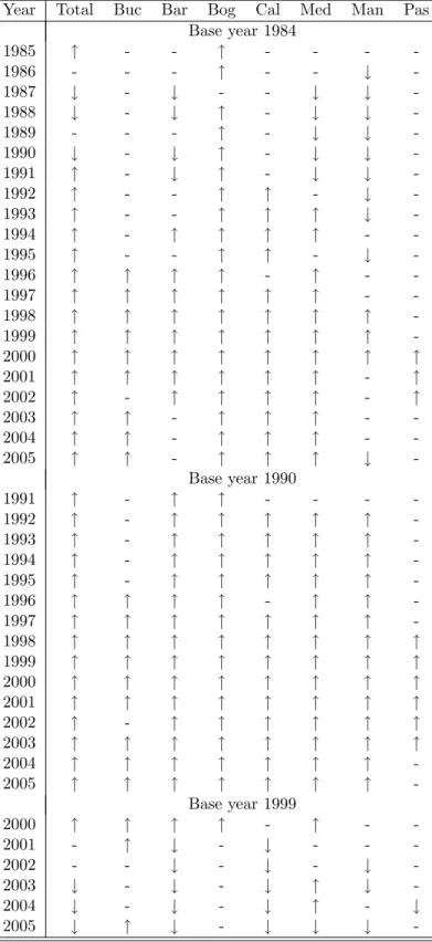
Table 3 compares the evolution of the Gini coe¢ cients for each city and for the country, with respect to three di¤erent base years: 1984, 1990 and 1999. The …rst base year is chosen simply because it is the beginning of our sample period. The second base year allows us to compare with respect to the year when the government introduced a series of structural policy measures aimed at liberalising Colombian trade and foreign exchange transactions, which were also accompanied by legislation to free the labour market while granting greater protection to union rights. The third base year allows us to provide a comparison with respect to the lowest point of the most serious recession recorded during the last century.
Let us consider …rst the results when using 1984 as base year. The cities of Barranquilla, Medellín and Manizales exhibit a downward trend in their Gini coef-…cients during the 1980s and early 1990s, which is subsequently reversed starting in the mid 1990s. In the case of Pasto, wage income distributions appear not to have changed with respect to the level observed in 1984. In the cases of Bogotá and the aggregate of the seven cities, the corresponding Gini coe¢ cients appear to have moved upwards. Using 1990 as base year, we …nd that most of the Gini coe¢ cients exhibit an increase, suggesting that the liberalising policy reforms of the early 1990s
6In the case of the city of Pasto, the estimated jackknife variance is almost 3 times the estimated
asymptotic variance. Jackknife estimates of the standard errors are not reported here for brevity, but are available from the authors upon request.
led to a worsening distribution of income. Lastly, when looking at the period that followed the deepest recession of the last century, evidence is somewhat mixed. The years of recovery do not appear to have had an e¤ect on wage income distribution in 21 out of the 48 comparisons provided, whereas in 18 cases there is a statistically signi…cant fall in the Gini coe¢ cients.
Overall, when assessing variations in the distributions of wage income with re-spect to 1990 and 1999, the picture that emerges is not particularly optimistic, in the sense that most of the observed variations in the Gini coe¢ cients are in the pos-itive direction (re‡ecting a worsening in inequality); it appears that the best-case scenario is that which re‡ects no statistically signi…cant variation at all.
4
Concluding remarks
This paper analyses the evolution of the Gini coe¢ cient in Colombia across cities, over a period of more than two decades. In order to provide valid inference on the observed variations of the estimated Gini coe¢ cients, we implement the David-son (2009) methodology to compute an asymptotically correct standard error. The estimated standard errors were used to perform hypotheses tests on wage income distribution equality across cities and over time. Focusing …rst on the cross section dimension, we …nd that there have been several years in which the observed dif-ferences in the Gini coe¢ cients at the city level do not turn out to be statistically di¤erent from zero. This highlights the importance of taking into account the coe¢ -cient estimated standard errors when performing comparisons. Turning to the time series dimension, we compare the corresponding Gini coe¢ cients for each city with the values observed in 1984, 1990 and 1999, and …nd that in most cases inequality has worsened.
References
Arango, L., A. García, and C. Posada (2006). La metodología de la encuesta continua de hogares y el empalme de la series del mercado laboral urbano de Colombia. Borradores de Economía No 410, Banco de la República.
Baer, W. and W. Maloney (1997). Neoliberalism and income distribution in Latin America. World Development 25, 311–327.
Berry, A. and M. Urrutia (1976). Income Distribution in Colombia. New Haven: Yale University Press.
Birchenall, J. (2001). Income distribution, human capital and economic growth in Colombia. Journal of Development Economics 66, 271–287.
Birchenall, J. (2007). Income distribution and macroeconomics in Colombia.Journal of Income Distribution 16, 6–24.
Cunningham , W., J. P. Jacobsen (2008). Earnings inequality within and across gender, racial, and ethnic groups in four Latin American countries. Policy Research Working Paper Series 4591. The World Bank.
Davidson, R. (2009). Reliable inference for the Gini index. Journal of Econometrics,
Journal of Econometrics 150, 30–40.
Davidson, R. and J. G. MacKinnon (1999).Econometric Theory and Methods. Ox-ford: Oxford University Press.
ECLAC (2006). Social panorama of Latin America. Retrieved on May 12, 2009 from http://www.eclac.org/publicaciones/.
ECLAC (2007). Social panorama of Latin America. Retrieved on May 12, 2009 from http://www.eclac.org/publicaciones/.
ECLAC (2008). Social panorama of Latin America. Retrieved on May 12, 2009 from http://www.eclac.org/publicaciones/.
Giles, D. (2004). Calculating a standard error for the Gini coe¢ cient: Some further results. Oxford Bulletin of Economics and Statistics 66, 425–433.
Giles, D. (2006). A cautionary note on estimating the standard error of the Gini index of inequality: Comment. Oxford Bulletin of Economics and Statistics 68, 395–396.
Lorenz, M. (1905). Methods of measuring the concentration of wealth. Publications of the American Statistical Association 9, 209–219.
Modarres, R. and J. Gastwirth (2006). A cautionary note on estimating the standard error of the Gini index of inequality. Oxford Bulletin of Economics and Statistics 68, 385–390.
Ocampo, J. A., F. Sánchez, and C. E. Tovar (2000). The labour market and income distribution in Colombia in the 1990s. CEPAL Review 72, 53–77.
Ogwang, T. (2000). A convenient method of computing the Gini index and its standard error. Oxford Bulletin of Economics and Statistics 62, 123–129.
Ogwang, T. (2004). Calculating a standard error for the Gini coe¢ cient: Some further results: Reply. Oxford Bulletin of Economics and Statistics 66, 435–437. Ogwang, T. (2006). A cautionary note on estimating the standard error of the Gini index of inequality: Comment. Oxford Bulletin of Economics and Statistics 68, 391–393.
Pyatt, G. (1976). On the interpretation and disaggregation of Gini coe¢ cients.
Economic Journal 86, 243–255.
Sen, A. (1973). On Economic Inequality. Oxford: Clarendon Press.
Urrutia, M. (1994). Colombia. In J. Williamson (Ed.), The Political Economy of Policy Reform, pp. 285–315. Washington, DC: Institute for International Economics.
Vélez, C. E. (1995). Gasto Social Y Desigualdad. Bogotá: Departamento Nacional de Planeación. Editorial Tercer Mundo Editores.
World Bank (2005). World Development Report 2006: Equity and Development. New York NY: Oxford University Press.
Zheng, B. and B. J. Cushing (2001). Statistical inference for testing inequality indices with dependent samples. Journal of Econometrics 101, 315–335.
T a b le 1 . T o ta l n u m b e r o f o b se rv a ti o n s, m e d ia n h o u rl y w a g e a n d st a n d a rd d e v ia ti o n (i n c o n st a n t p ri c e s o f 2 0 0 5 ) Y e a r T o ta l B o g B a r B u c C a l M e d M a n P a s O b s M e d ia n S D M e d ia n S D M e d ia n S D M e d ia n S D M e d ia n S D M e d ia n S D M e d ia n S D M e d ia n S D 1 9 8 4 7 6 9 4 6 1 ,8 7 9 3 ,4 3 3 1 ,9 8 7 3 ,4 1 2 1 ,8 7 9 3 ,9 7 3 1 ,7 8 6 2 ,6 5 4 1 ,8 9 2 3 ,2 2 6 1 ,8 0 3 3 ,5 9 5 1 ,7 6 9 2 ,7 3 9 1 ,5 3 1 3 ,1 2 3 1 9 8 5 5 6 1 3 0 1 ,7 2 6 4 ,0 0 5 1 ,8 4 1 3 ,8 2 1 1 ,7 8 2 3 ,2 8 3 1 ,5 8 2 2 ,5 9 9 1 ,6 5 6 5 ,3 5 0 1 ,7 1 1 4 ,5 5 4 1 ,5 8 4 2 ,6 9 6 1 ,4 6 1 2 ,2 6 1 1 9 8 6 5 9 4 6 9 1 ,7 3 0 4 ,0 9 6 1 ,9 2 2 4 ,2 1 1 1 ,7 1 9 3 ,2 5 0 1 ,6 8 5 2 ,2 1 9 1 ,7 0 9 2 ,8 9 1 1 ,6 8 5 5 ,5 6 2 1 ,6 8 8 2 ,3 6 9 1 ,5 3 8 2 ,3 0 0 1 9 8 7 6 2 4 1 4 1 ,7 3 3 3 ,0 4 1 1 ,8 3 6 3 ,4 7 3 1 ,6 8 2 2 ,3 8 0 1 ,6 5 3 2 ,1 1 8 1 ,8 0 3 4 ,0 4 1 1 ,7 0 3 2 ,3 0 6 1 ,6 5 3 2 ,8 5 4 1 ,5 4 5 2 ,5 6 1 1 9 8 8 6 5 1 5 3 1 ,6 5 5 2 ,9 2 7 1 ,7 5 8 3 ,9 1 5 1 ,5 5 1 1 ,9 9 8 1 ,5 8 9 2 ,3 6 6 1 ,6 9 8 2 ,8 0 3 1 ,6 3 0 2 ,2 4 9 1 ,6 0 1 2 ,3 3 9 1 ,4 9 4 2 ,2 1 0 1 9 8 9 6 6 1 4 7 1 ,6 7 7 3 ,9 5 5 1 ,7 8 6 5 ,8 4 5 1 ,6 5 1 2 ,3 6 5 1 ,5 7 6 3 ,7 7 0 1 ,7 3 2 2 ,9 5 3 1 ,6 2 9 2 ,5 8 6 1 ,6 5 1 2 ,2 6 3 1 ,5 0 0 2 ,3 8 3 1 9 9 0 5 8 1 5 2 1 ,6 7 3 2 ,8 5 5 1 ,7 6 5 3 ,7 5 2 1 ,6 6 9 2 ,4 3 5 1 ,5 8 6 2 ,2 5 1 1 ,6 8 1 2 ,9 8 4 1 ,6 6 9 2 ,1 4 4 1 ,6 0 3 1 ,9 1 2 1 ,4 8 8 2 ,3 3 0 1 9 9 1 5 7 8 0 4 1 ,6 1 7 3 ,5 1 4 1 ,7 5 4 4 ,4 7 5 1 ,5 9 6 2 ,0 9 6 1 ,5 2 7 2 ,1 8 6 1 ,6 9 4 5 ,1 5 6 1 ,5 9 6 2 ,4 8 5 1 ,5 7 9 2 ,0 7 1 1 ,4 4 4 2 ,2 2 3 1 9 9 2 5 9 8 0 8 1 ,5 9 6 4 ,3 0 3 1 ,6 8 9 4 ,0 5 2 1 ,5 7 6 8 ,4 6 9 1 ,5 2 7 2 ,0 3 9 1 ,6 7 3 2 ,9 9 9 1 ,5 7 6 2 ,3 9 2 1 ,5 2 7 2 ,8 0 4 1 ,3 6 9 2 ,0 5 8 1 9 9 3 6 0 1 3 4 1 ,6 3 7 7 ,5 7 0 1 ,6 8 3 1 0 ,5 6 4 1 ,6 1 1 4 ,7 9 7 1 ,5 6 7 2 ,6 2 7 1 ,7 6 3 1 0 ,4 3 2 1 ,6 3 2 5 ,7 1 1 1 ,5 3 5 2 ,3 7 0 1 ,5 7 8 2 ,3 6 7 1 9 9 4 6 7 2 0 3 1 ,7 4 7 6 ,9 7 3 1 ,9 0 1 8 ,9 8 3 1 ,6 3 8 8 ,9 3 4 1 ,6 4 2 3 ,7 0 2 1 ,8 8 1 4 ,0 8 0 1 ,6 3 8 6 ,2 3 7 1 ,5 8 4 3 ,2 7 6 1 ,5 2 6 2 ,4 8 4 1 9 9 5 6 1 4 4 2 1 ,7 0 2 4 ,5 9 0 1 ,9 1 6 6 ,6 6 9 1 ,6 7 2 2 ,9 5 0 1 ,6 3 1 2 ,6 0 4 1 ,8 6 5 5 ,3 6 7 1 ,6 7 2 2 ,7 8 8 1 ,5 2 3 2 ,2 4 5 1 ,4 2 4 2 ,5 3 5 1 9 9 6 6 1 6 9 1 1 ,7 1 6 4 ,7 0 7 1 ,9 7 4 5 ,4 1 7 1 ,8 1 6 3 ,0 4 9 1 ,6 4 7 3 ,2 0 2 1 ,6 8 5 2 ,9 4 3 1 ,5 9 0 6 ,2 2 1 1 ,6 3 4 3 ,5 2 0 1 ,5 6 9 4 ,4 2 0 1 9 9 7 5 7 1 4 5 1 ,7 4 8 5 ,0 6 5 2 ,2 9 7 9 ,3 7 9 1 ,8 3 8 3 ,3 6 4 1 ,6 6 0 3 ,1 2 7 1 ,6 2 3 4 ,4 9 6 1 ,6 5 7 4 ,6 8 8 1 ,5 8 5 3 ,4 9 0 1 ,6 2 8 3 ,2 0 6 1 9 9 8 5 4 1 0 4 1 ,7 6 1 4 ,6 2 6 2 ,1 3 6 7 ,3 5 8 1 ,8 7 2 3 ,4 5 8 1 ,6 8 2 4 ,3 3 9 1 ,7 1 6 4 ,2 0 3 1 ,6 6 8 4 ,1 7 9 1 ,6 8 2 3 ,4 0 3 1 ,5 6 4 3 ,1 0 4 1 9 9 9 4 6 2 8 7 1 ,7 2 0 4 ,1 3 7 1 ,9 5 6 5 ,7 2 5 1 ,7 2 9 3 ,1 3 3 1 ,6 5 2 2 ,7 9 0 1 ,7 1 8 4 ,6 1 1 1 ,6 6 3 3 ,1 7 4 1 ,7 7 1 4 ,2 6 1 1 ,5 9 7 4 ,0 2 9 2 0 0 0 4 4 6 6 0 1 ,6 1 9 5 ,8 7 4 1 ,8 0 2 9 ,8 4 6 1 ,6 7 7 4 ,0 6 7 1 ,5 7 2 7 ,3 7 1 1 ,6 1 5 3 ,5 7 7 1 ,5 7 7 4 ,4 7 0 1 ,6 7 7 4 ,4 6 9 1 ,5 0 9 3 ,2 9 3 2 0 0 1 4 2 3 3 9 2 ,0 5 1 4 ,5 7 6 2 ,1 2 2 6 ,9 6 4 2 ,1 9 1 3 ,8 5 2 1 ,9 6 4 3 ,7 1 0 2 ,0 6 8 4 ,1 1 9 2 ,0 3 4 4 ,2 9 9 2 ,0 8 9 4 ,2 5 0 1 ,9 4 2 3 ,5 1 1 2 0 0 2 4 1 5 7 3 2 ,0 7 3 6 ,7 9 7 2 ,2 2 1 1 5 ,0 4 7 2 ,2 1 0 3 ,4 9 2 2 ,0 0 8 3 ,0 5 9 2 ,0 9 5 4 ,4 7 3 2 ,0 5 7 3 ,6 7 2 2 ,0 2 7 3 ,3 3 9 2 ,0 4 5 3 ,7 8 3 2 0 0 3 4 1 0 0 8 2 ,0 1 8 4 ,1 1 0 2 ,1 4 9 5 ,2 5 5 2 ,0 1 4 4 ,0 7 2 1 ,9 6 1 3 ,1 4 2 2 ,0 2 0 3 ,7 6 4 2 ,0 4 8 4 ,6 8 6 2 ,0 4 8 3 ,5 2 4 1 ,9 7 5 3 ,5 5 5 2 0 0 4 4 2 0 6 9 2 ,0 6 9 5 ,4 7 6 2 ,1 8 5 6 ,8 4 2 2 ,0 6 9 3 ,1 2 4 2 ,0 3 6 3 ,2 1 1 2 ,0 8 1 4 ,5 3 5 2 ,0 8 6 4 ,8 7 1 2 ,0 5 7 8 ,6 3 7 2 ,0 4 8 3 ,1 3 7 2 0 0 5 4 8 0 6 2 2 ,1 2 7 4 ,4 9 3 2 ,3 1 9 6 ,6 5 5 2 ,2 3 5 3 ,8 6 6 1 ,9 8 6 3 ,8 0 3 2 ,1 4 5 4 ,5 2 9 2 ,1 3 4 4 ,0 1 0 2 ,0 9 8 3 ,2 6 0 2 ,0 0 0 3 ,5 7 3 S o u rc e : A u th o rs c a lc u la ti o n s b a se d o n h o u se h o ld su rv e y d a ta .
Table 2. Number of times the Gini coe¢ cients are equal (1984 - 2005) City Bar Bog Cal Med Man Pas
Buc 11 1 12 14 10 0 Bar 3 9 11 7 2 Bog 4 0 2 8 Cal 6 16 3 Med 7 0 Man 3
Table 3. Statistically signi…cant variations in Gini coe¢ cients Year Total Buc Bar Bog Cal Med Man Pas
Base year 1984 1985 " - - " - - - -1986 - - - " - - # -1987 # - # - - # # -1988 # - # " - # # -1989 - - - " - # # -1990 # - # " - # # -1991 " - # " - # # -1992 " - - " " - # -1993 " - - " " " # -1994 " - " " " " - -1995 " - - " " - # -1996 " " " " - " - -1997 " " " " " " - -1998 " " " " " " " -1999 " " " " " " " -2000 " " " " " " " " 2001 " " " " " " - " 2002 " - " " " " - " 2003 " " - " " " - -2004 " " - " " " - -2005 " " - " " " # -Base year 1990 1991 " - " " - - - -1992 " - " " " " " -1993 " - " " " " " -1994 " - " " " " " -1995 " - " " " " " -1996 " " " " - " " -1997 " " " " " " " -1998 " " " " " " " " 1999 " " " " " " " " 2000 " " " " " " " " 2001 " " " " " " " " 2002 " - " " " " " " 2003 " " " " " " " " 2004 " " " " " " " -2005 " " " " " " " -Base year 1999 2000 " " " " - " - -2001 - " # - # - - -2002 - - # - # - # -2003 # - # - # " # -2004 # - # - # " - # 2005 # " # - # # #
-Appendix 1. Estimates, standard errors and con…dence intervals of the Gini coe¢ cient
Year Total Bogotá
Con…dence interval based on: Con…dence interval based on:
Gini (s.e.) N(0;1) Bootstrap Gini (s.e.) N(0;1) Bootstrap
Lower Upper lower upper lower upper lower upper
1984 0.405 0.0021 0.401 0.409 0.401 0.409 0.413 0.0028 0.407 0.418 0.408 0.419 1985 0.420 0.0032 0.414 0.426 0.416 0.425 0.429 0.0043 0.420 0.437 0.423 0.435 1986 0.406 0.0033 0.399 0.412 0.401 0.411 0.428 0.0048 0.419 0.437 0.422 0.434 1987 0.389 0.0024 0.385 0.394 0.386 0.392 0.416 0.0039 0.408 0.424 0.412 0.420 1988 0.396 0.0022 0.391 0.400 0.393 0.399 0.432 0.0045 0.424 0.441 0.426 0.439 1989 0.398 0.0032 0.391 0.404 0.393 0.403 0.430 0.0075 0.415 0.445 0.420 0.444 1990 0.395 0.0022 0.391 0.400 0.393 0.397 0.434 0.0044 0.425 0.443 0.431 0.437 1991 0.412 0.0028 0.406 0.418 0.409 0.415 0.462 0.0051 0.452 0.472 0.459 0.466 1992 0.419 0.0037 0.412 0.426 0.414 0.424 0.453 0.0046 0.444 0.462 0.450 0.456 1993 0.456 0.0057 0.445 0.467 0.447 0.467 0.513 0.0117 0.490 0.536 0.498 0.530 1994 0.465 0.0046 0.456 0.473 0.457 0.473 0.513 0.0079 0.497 0.529 0.500 0.529 1995 0.434 0.0033 0.428 0.441 0.431 0.438 0.478 0.0071 0.464 0.492 0.470 0.486 1996 0.442 0.0033 0.436 0.449 0.439 0.446 0.466 0.0063 0.454 0.478 0.461 0.470 1997 0.458 0.0034 0.451 0.465 0.455 0.461 0.517 0.0109 0.496 0.539 0.508 0.526 1998 0.466 0.0029 0.460 0.471 0.464 0.468 0.514 0.0080 0.498 0.529 0.508 0.519 1999 0.462 0.0027 0.456 0.467 0.460 0.463 0.503 0.0067 0.490 0.516 0.500 0.506 2000 0.486 0.0043 0.478 0.495 0.483 0.489 0.538 0.0133 0.512 0.564 0.528 0.548 2001 0.458 0.0026 0.453 0.463 0.456 0.459 0.505 0.0083 0.488 0.521 0.500 0.508 2002 0.457 0.0048 0.447 0.466 0.453 0.460 0.530 0.0190 0.492 0.567 0.511 0.547 2003 0.449 0.0025 0.444 0.454 0.448 0.450 0.490 0.0061 0.478 0.502 0.488 0.491 2004 0.450 0.0037 0.443 0.458 0.448 0.453 0.511 0.0076 0.496 0.526 0.508 0.514 2005 0.442 0.0025 0.437 0.447 0.440 0.443 0.502 0.0065 0.489 0.515 0.499 0.505
Appendix 1 (continued). Estimates, standard errors and con…dence intervals of the Gini coe¢ cient
Year Barranquilla Bucaramanga
Con…dence interval based on: Con…dence interval based on:
Gini (s.e.) N(0;1) Bootstrap Gini (s.e.) N(0;1) Bootstrap
Lower Upper lower upper lower upper lower upper
1984 0.396 0.0087 0.379 0.413 0.382 0.422 0.387 0.0075 0.372 0.402 0.375 0.406 1985 0.408 0.0076 0.393 0.423 0.400 0.416 0.400 0.0076 0.385 0.414 0.386 0.417 1986 0.411 0.0070 0.397 0.424 0.403 0.419 0.379 0.0060 0.367 0.390 0.367 0.391 1987 0.363 0.0062 0.350 0.375 0.357 0.369 0.376 0.0053 0.365 0.386 0.366 0.387 1988 0.355 0.0053 0.345 0.366 0.351 0.359 0.396 0.0055 0.385 0.407 0.386 0.407 1989 0.377 0.0053 0.367 0.388 0.368 0.389 0.406 0.0104 0.386 0.426 0.391 0.444 1990 0.352 0.0061 0.340 0.364 0.343 0.362 0.389 0.0054 0.378 0.399 0.381 0.397 1991 0.369 0.0044 0.360 0.377 0.364 0.374 0.388 0.0052 0.378 0.398 0.380 0.396 1992 0.412 0.0221 0.369 0.455 0.381 0.554 0.376 0.0050 0.366 0.386 0.370 0.382 1993 0.414 0.0112 0.392 0.436 0.395 0.444 0.396 0.0063 0.384 0.409 0.385 0.411 1994 0.478 0.0163 0.446 0.510 0.451 0.524 0.395 0.0094 0.377 0.414 0.381 0.423 1995 0.414 0.0055 0.403 0.425 0.410 0.418 0.393 0.0058 0.381 0.404 0.388 0.398 1996 0.418 0.0050 0.409 0.428 0.415 0.422 0.426 0.0064 0.413 0.438 0.414 0.440 1997 0.426 0.0056 0.415 0.437 0.421 0.430 0.432 0.0058 0.420 0.443 0.424 0.439 1998 0.434 0.0053 0.424 0.445 0.430 0.438 0.445 0.0089 0.428 0.463 0.433 0.458 1999 0.436 0.0048 0.427 0.446 0.434 0.439 0.409 0.0064 0.397 0.422 0.405 0.414 2000 0.468 0.0071 0.454 0.482 0.464 0.473 0.464 0.0194 0.426 0.502 0.439 0.496 2001 0.420 0.0054 0.409 0.430 0.417 0.423 0.449 0.0060 0.438 0.461 0.444 0.454 2002 0.416 0.0051 0.406 0.426 0.413 0.418 0.403 0.0062 0.391 0.415 0.399 0.408 2003 0.411 0.0083 0.395 0.428 0.406 0.416 0.426 0.0056 0.415 0.437 0.421 0.430 2004 0.379 0.0064 0.366 0.391 0.376 0.381 0.418 0.0060 0.406 0.430 0.413 0.422 2005 0.383 0.0077 0.368 0.398 0.378 0.388 0.444 0.0061 0.432 0.455 0.437 0.449
Appendix 1 (continued). Estimates, standard errors and con…dence intervals of the Gini coe¢ cient
Year Cali Medellín
Con…dence interval based on: Con…dence interval based on:
Gini (s.e.) N(0;1) Bootstrap Gini (s.e.) N(0;1) Bootstrap
Lower Upper lower upper lower upper lower upper
1984 0.402 0.0051 0.392 0.412 0.400 0.404 0.375 0.0056 0.364 0.386 0.371 0.379 1985 0.424 0.0125 0.400 0.449 0.416 0.431 0.393 0.0088 0.376 0.411 0.386 0.399 1986 0.392 0.0056 0.381 0.403 0.390 0.394 0.367 0.0113 0.345 0.389 0.356 0.377 1987 0.409 0.0078 0.394 0.424 0.405 0.412 0.322 0.0044 0.314 0.331 0.320 0.324 1988 0.395 0.0052 0.385 0.406 0.394 0.397 0.336 0.0038 0.329 0.344 0.335 0.338 1989 0.398 0.0053 0.388 0.409 0.397 0.400 0.328 0.0052 0.318 0.338 0.325 0.331 1990 0.397 0.0061 0.385 0.409 0.395 0.399 0.341 0.0039 0.333 0.349 0.340 0.342 1991 0.418 0.0116 0.395 0.440 0.410 0.423 0.349 0.0049 0.339 0.358 0.347 0.351 1992 0.418 0.0055 0.408 0.429 0.417 0.420 0.372 0.0042 0.364 0.380 0.370 0.373 1993 0.475 0.0186 0.439 0.512 0.456 0.494 0.414 0.0104 0.394 0.434 0.404 0.423 1994 0.425 0.0072 0.411 0.439 0.422 0.428 0.421 0.0106 0.401 0.442 0.411 0.431 1995 0.431 0.0106 0.410 0.452 0.425 0.437 0.378 0.0048 0.369 0.388 0.376 0.380 1996 0.408 0.0060 0.396 0.420 0.407 0.410 0.430 0.0100 0.410 0.450 0.420 0.439 1997 0.441 0.0096 0.423 0.460 0.437 0.445 0.426 0.0074 0.412 0.441 0.422 0.431 1998 0.451 0.0077 0.436 0.466 0.448 0.454 0.437 0.0067 0.423 0.450 0.434 0.440 1999 0.476 0.0079 0.461 0.492 0.473 0.479 0.416 0.0053 0.405 0.426 0.414 0.417 2000 0.456 0.0068 0.443 0.470 0.455 0.458 0.466 0.0075 0.452 0.481 0.463 0.469 2001 0.449 0.0065 0.437 0.462 0.448 0.451 0.418 0.0067 0.405 0.432 0.416 0.421 2002 0.453 0.0072 0.439 0.467 0.451 0.455 0.413 0.0056 0.402 0.424 0.412 0.415 2003 0.429 0.0068 0.416 0.443 0.428 0.431 0.448 0.0064 0.435 0.461 0.445 0.450 2004 0.446 0.0078 0.430 0.461 0.443 0.448 0.434 0.0067 0.421 0.447 0.431 0.437 2005 0.449 0.0065 0.437 0.462 0.447 0.452 0.398 0.0053 0.387 0.408 0.395 0.400
Appendix 1 (continued). Estimates, standard errors and con…dence intervals of the Gini coe¢ cient
Year Manizales Pasto
Con…dence interval based on: Con…dence interval based on:
Gini (s.e.) N(0;1) Bootstrap Gini (s.e.) N(0;1) Bootstrap
Lower Upper lower upper lower upper lower upper
1984 0.436 0.0076 0.421 0.451 0.435 0.437 0.464 0.0096 0.446 0.483 0.463 0.466 1985 0.437 0.0092 0.419 0.455 0.436 0.438 0.455 0.0058 0.444 0.466 0.454 0.456 1986 0.403 0.0079 0.388 0.419 0.402 0.404 0.445 0.0069 0.432 0.459 0.445 0.446 1987 0.404 0.0110 0.382 0.425 0.402 0.405 0.454 0.0078 0.438 0.469 0.453 0.454 1988 0.401 0.0072 0.387 0.415 0.400 0.402 0.447 0.0060 0.435 0.459 0.446 0.447 1989 0.393 0.0065 0.381 0.406 0.393 0.394 0.449 0.0069 0.435 0.462 0.448 0.450 1990 0.374 0.0055 0.363 0.385 0.374 0.375 0.459 0.0062 0.447 0.472 0.459 0.460 1991 0.379 0.0066 0.366 0.392 0.378 0.379 0.453 0.0070 0.439 0.466 0.452 0.453 1992 0.407 0.0097 0.388 0.426 0.405 0.408 0.449 0.0063 0.437 0.462 0.449 0.450 1993 0.406 0.0070 0.393 0.420 0.406 0.407 0.443 0.0062 0.431 0.455 0.442 0.444 1994 0.427 0.0104 0.406 0.447 0.424 0.429 0.451 0.0060 0.439 0.463 0.450 0.451 1995 0.409 0.0057 0.398 0.420 0.408 0.409 0.458 0.0064 0.445 0.470 0.457 0.459 1996 0.446 0.0076 0.431 0.460 0.443 0.447 0.475 0.0109 0.454 0.496 0.472 0.477 1997 0.451 0.0064 0.438 0.463 0.449 0.453 0.469 0.0061 0.457 0.481 0.468 0.470 1998 0.456 0.0055 0.445 0.467 0.455 0.457 0.481 0.0052 0.471 0.491 0.480 0.482 1999 0.466 0.0075 0.451 0.480 0.463 0.468 0.488 0.0085 0.471 0.504 0.485 0.489 2000 0.469 0.0091 0.451 0.486 0.465 0.471 0.504 0.0057 0.493 0.515 0.503 0.505 2001 0.454 0.0065 0.442 0.467 0.452 0.456 0.489 0.0047 0.480 0.499 0.489 0.490 2002 0.441 0.0049 0.432 0.451 0.440 0.442 0.488 0.0047 0.479 0.498 0.488 0.489 2003 0.433 0.0056 0.422 0.444 0.431 0.434 0.478 0.0054 0.467 0.488 0.477 0.479 2004 0.454 0.0173 0.420 0.488 0.440 0.465 0.456 0.0049 0.446 0.465 0.455 0.456 2005 0.407 0.0054 0.397 0.418 0.406 0.409 0.473 0.0059 0.461 0.484 0.472 0.473