Vol. 00, No. 00, Month 20XX, 1–24
Computing the Shapley Value in Allocation Problems: Approximations and
Bounds, with an Application to the Italian VQR Research Assessment
Program
Francesco Lupiaa†, Angelo Mendicellia‡, Andrea Ribichinib§, Francesco ScarcelloaP and Marco Schaerfc,dk
aDept. of Computer Science, Modeling, Electronics and Systems Engineering, University of Calabria,
87036, Rende, Italy;bDept. of Physics, Sapienza University of Rome, 00185, Rome, Italy;cDept. of
Computer, Control, and Management Engineering “Antonio Ruberti”, Sapienza University of Rome, 00185, Rome, Italy;dInstitute of Information Technologies and Telecommunications, North Caucasus
Federal University, Stavropol, Russian Federation
(Received 00 Month 20XX; final version received 00 Month 20XX)
In allocation problems, a given set of goods are assigned to agents in such a way that the social welfare is maximised, that is, the largest possible global worth is achieved. When goods are indivisible, it is pos-sible to use money compensation to perform a fair allocation taking into account the actual contribution of all agents to the social welfare. Coalitional games provide a formal mathematical framework to model such problems, in particular the Shapley value is a solution concept widely used for assigning worths to agents in a fair way. Unfortunately, computing this value is a#P-hard problem, so that applying this good theoretical notion is often quite difficult in real-world problems.
We describe useful properties that allow us to greatly simplify the instances of allocation problems, without affecting the Shapley value of any player. Moreover, we propose algorithms for computing lower bounds and upper bounds of the Shapley value, which in some cases provide the exact result and that can be combined with approximation algorithms.
The proposed techniques have been implemented and tested on a real-world application of allocation problems, namely, the Italian research assessment program known as VQR (Verifica della Qualit`a della Ricerca, or Research Quality Assessment)1. For the large university considered in the experiments, the problem involves thousands of agents and goods (here, researchers and their research products). The algorithms described in the paper are able to compute the Shapley value for most of those agents, and to get a good approximation of the Shapley value for all of them2.
Keywords:Coalitional games; Allocation problems; Game theory; Shapley value computation; Approximation algorithms; Research assessment exercises
†Email: [email protected] ‡Email: [email protected] §Email: [email protected]
PCorresponding author. Email: [email protected] kEmail: [email protected]
1We refer the interested reader to the web site of the Italian National Agency for the Evaluation of Universities and Research Institutes (ANVUR):http://www.anvur.org/
2A preliminary version of this article was presented at RCRA 2016 (Lupia, Mendicelli, Ribichini, Scarcello, & Schaerf, 2016). The current version makes use of a new algorithm in order to improve the Shapley value approximation, besides providing formal proofs and a more detailed presentation.
1. Introduction
1.1. Coalitional Game Theory
Coalitional games provide a rich mathematical framework to analyze interactions between in-telligent agents (see, e.g., Osborne & Rubinstein, 1994). We consider coalitional games of the form G = hN, vi, consisting of a set N ofnagents and a characteristic functionv. The latter maps each coalitionC ⊆N to the worth that agents inCcan obtain by collaborating with each other. In this context, the crucial problem is to find a mechanism to allocate the worthv(N), i.e., the value of the grand-coalitionN, in a way that is fair for all players and that additionally satis-fies some further important properties such as efficiency (i.e., distributing precisely the available budgetv(N)to players, not more and not less). Moreover, for fairness and stability reasons, it is usually required that every group of agentsCgets at least the worthv(C)that it can guarantee to the game.
Several solution concepts have been considered in the literature as “fair allocation” schemes and, among them, a prominent one is the Shapley value (Shapley, 1953). According to this notion, the worth of any agent iis determined by considering its actual contribution to all the possible coalitions of agents.
1.2. Allocation Games
Among the various classes of coalitional games, we focus in this paper on allocation games, which is a setting for analyzing fair division problems where monetary compensations are al-lowed and utilities are quasi-linear (Moulin, 1992). Allocation games naturally arise in various application domains, ranging from house allocation to room assignment and rent division, to (cooperative) scheduling and task allocation, to protocols for wireless communication networks, and to queuing problems (see, e.g., Greco & Scarcello, 2014b; Iera, Militano, Romeo, & Scar-cello, 2011; Maniquet, 2003; Mishra & Rangarajan, 2007; Moulin, 1992, and the references therein).
Computing the Shapley value of such games is a difficult problem, indeed it is #P-hard even if goods can only have two different possible values (Greco, Lupia, & Scarcello, 2015). In this paper we focus on large instances of this problem, involving thousands of agents and goods, for which no algorithm described in the literature is able to provide an exact solution. We point out that there are, however, some promising recent advances that identify islands of tractabil-ity for the allocation problems where at most one good is allocated to each agent: it has been recently shown that those instances where the treewidth(Robertson & Seymour, 1984) of the agents’ interaction-graph is bounded by some constant (i.e., instances that exhibit a low degree of cyclicity) can be solved in polynomial-time (Greco et al., 2015). The result is based on re-cent advances on counting solutions of conjunctive queries with existential variables (Greco & Scarcello, 2014a). Unfortunately, if the structure is quite cyclic this technique cannot be applied to large instances, because its computational complexity has an exponential dependency on the treewidth.
In some applications, one can be satisfied with approximations of the Shapley value. With this respect, things are quite good in principle, since we know there exists a fully polynomial-time randomized approximation scheme to compute the Shapley value in supermod-ular games (Liben-Nowell, Sharp, Wexler, & Woods, 2012). The algorithm can thus be tuned to obtain the desired maximum expected error, as a percentage of the correct Shapley value, and it can be used for the allocation games we consider in this paper. However, not very surprisingly, for very large instances one has to consider a huge number of samples, in order to stay below a reasonable expected error. Maleki, Tran-Thanh, Hines, Rahwan, and Rogers (2013) provide
bounds for the estimation error (as an absolute number rather than a percentage of the correct value) if the variance or the range of the samples are known. They also introduce stratified sampling as a method to further reduce the number of required samples. Other approximation efforts based on sampling methods include the work of Castro, G´omez, and Tejada (2009). How-ever, they bound the number of required samples using the Central Limit Theorem (Stein, 1972), which only holds when the number of samples increases to infinity. Therefore, it has been argued that their bound is not accurate (Maleki et al., 2013).
1.3. Contribution
In order to attack large instances of allocation problems, we start by proving some useful prop-erties of these problems that allow us to decompose instances into smaller pieces, which can be solved independently. Moreover, some of these properties identify cases where the computation of the worth function can be obtained in a very efficient way.
With these properties, we are able to use the randomized approximation algorithm of Liben-Nowell et al. (2012) even on instances that (when not decomposed) are very large (see Sec-tion 6.1 for a brief descripSec-tion of the approximaSec-tion algorithm, and SecSec-tion 7.2 for our experi-mental results).
Furthermore, we note that in some applications one may prefer to determine a guaranteed interval for the Shapley value, rather than one probably good point. Therefore, we propose al-gorithms for computing a lower bound and an upper bound of the Shapley value for allocation problems. In many cases the distance between the two bounds is quite small, and sometimes they even coincide, which means that we actually computed the exact value. We also used these algorithms together with the approximation algorithm of Liben-Nowell et al. (2012), to provide a more accurate evaluation of the maximum error of this randomized solution, for the considered instances.
Moreover, by plugging the computed lower bound values into the randomized sampling algo-rithm proposed by Maleki et al. (2013), we were able to express their error bound as a percentage of the correct Shapley value, rather than as an absolute number, at least for our test instances. This allowed us to compute approximate Shapley values for our largest test case (namely, the 2011-2014 research assessment exercise of Sapienza University of Rome), within 5% of the cor-rect value with 99% probability, in a matter of hours (we refer the reader to Section 6.2 for a brief description of Maleki et al.’s algorithm, and Section 7.2 for our experimental results).
1.4. The Case Study
We have tested the proposed techniques on large real-world instances of the VQR2011-2014 Italian research assessment exercise. This exercise requires every Italian research structure R
to select some research products, and submit them to an evaluation agency called ANVUR. While doing so, the structureR is in competition with all other Italian research structures, as the outcome of the evaluation will be used to proportionally transfer the funds allocated by the Ministry to support research activities in the next years (until the subsequent evaluation process). Every structureR is therefore interested in selecting and submitting its best research products. For the sake of simplicity, we next simply speak of publications instead of research products (which can also be patents, books, etc.), and of universities and departments instead of structures and substructures (which can be other research subjects). The programme is articulated in two phases: (1) Based on authors’ self-evaluations and on ANVUR guidelines,Rselects and submits
to ANVUR (at most) two publications for each one of its authors3, in such a way that any product is formally associated with at most one author. (2) ANVUR formulates its independent quality judgment about the submitted publications (the score assigned to each publication is currently made known only to its authors), and the sum of the scores resulting from ANVUR’s evaluation is then the VQR score of R. Eventually,R will receive funds in subsequent years proportional to this score. Furthermore, ANVUR also published an evaluation of all departments, based on the product scores (the score of each department was computed as the sum of the scores of the products formally assigned to the authors in that department). Finally, the scores were also used for evaluating individual researchers that had been recently hired by R (this also greatly influenced R’s funds in subsequent years), as well as those researchers that were members of PhD committees. Scores for recently hired researchers were computed as the sum of the scores of the products formally assigned to them; data in this respect were published by ANVUR in aggregated form only, for each department and for each scientific disciplinary sector. Evaluations for researchers that were members of PhD committees were computed as the sum of the scores of the best publications each one of them had coauthored, among all the publications submitted for the VQR (for this evaluation, the formal assignment of publications to authors was irrelevant); data in this respect were published by ANVUR in aggregated form only, for each PhD committee.
The way ANVUR currently uses product scores, for the purposes described above, yields evaluations that do not satisfy the desirable properties outlined in Section 4. In order to deal with this issue, we have modeled the problem as an allocation game (Greco & Scarcello, 2013), with a fair way to divide the total score of the university among researchers, groups, and departments based on the Shapley value. The proposed division rule enjoys many desirable properties, such as the independence of the specific allocation of research products, the independence of the preliminary (optimal) products selection, the guarantee of the actual (marginal) contribution, and so on.
2. Preliminaries
2.1. Allocation scenario and its associated game
In the setting considered in this paper, a game is defined by an allocation scenario A =
hN,G,Ω,val, kicomprising a set of agentsN and a set of goodsG, whose values are given by
the functionvalmapping each good to a non-negative real number. The functionΩassociates each agent with the set of goods he/she is interested in. Moreover, the natural numberkprovides the maximum number of goods that can be assigned to each agent. Each good is indivisible and can be assigned at most to one player.
For a coalitionC ⊆ N, a (feasible) allocation πA[C]is a mapping fromC to sets of goods from Gsuch that: each agent i ∈ C gets a set of goodsπA(i) ⊆ Ω(i) with|πA(i)| ≤ k, and πA(i)∩πA(j) =∅, for any other agentj∈C(each good can be assigned to one agent at most). We denote byimg(πA[C])the set of all goods in the image ofπA[C], that is,img(πA[C]) =
S
i∈CπA[C](i). With a slight abuse of notation, we denote byval(S)the sum of all the values
of a set of goodsS⊆G, and byval(πA[C])the valueval(img(πA[C])). An allocationπA[C]
is optimal if there exists no allocationπA0 [C]withval(πA0 [C]) >val(πA[C]). The total value of such an optimal allocation for the coalition Cis denoted byoptA(C). The budget available
forA, also called the (maximum) social welfare, isoptA(N), that is, the value of any optimal
allocation for the whole set of agents N (the grand-coalition). The coalitional game defined by
3There are exceptions to this rule: in specific circumstances, fewer than two publications are expected for some authors. To our ends, this detail is immaterial.
the scenarioAis the pairhN,optAi, that is, the game where the worth of any coalition is given
by the value of any of its optimal allocations. Note thatoptA(C) ≥ 0holds for eachC ⊆N, since the allocation where no agent receives any goods is a feasible one (the value of an empty set of goods is0). The definition trivializes forC=∅, withoptA(∅) = 0.
g
1g
2g
3g
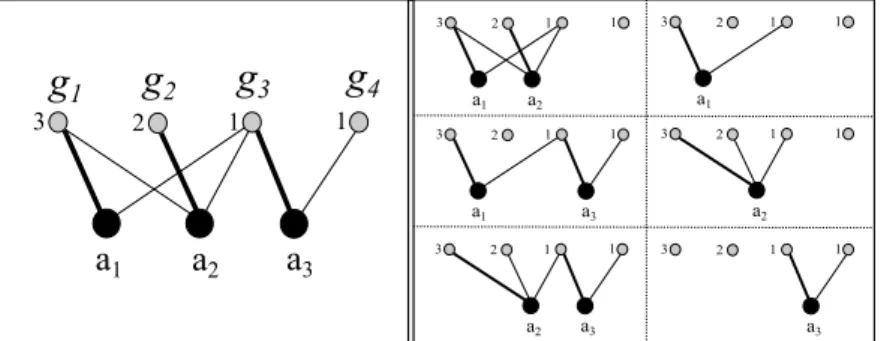
4 a1 a2 a3 3 2 1 1 a1 a2 3 2 1 1 a1 a3 3 2 1 1 a2 a3 3 2 1 1 a1 3 2 1 1 a2 3 2 1 1 a3 3 2 1 1Figure 1.: Allocation scenarioA0 in Example 2.1.
Example 2.1: Consider the allocation scenarioA0 =h{a1, a2, a3},{g1, g2, g3, g4},Ω,val,1i,
depicted in a graphical way in Figure 1, where each edge connects an agent to a good he/she is interested in, and it is possible to allocate just one good to each agent (k= 1). The figure shows on the left an allocation for all the agents, with the edges in bold identifying the allocation of goods to agents. Note that this is an optimal allocation, i.e., a feasible allocation whose sum of values of the allocated goods is the maximum possible one. The value of this allocation is
val(g1) +val(g2) +val(g3) = 3 + 2 + 1 = 6.
The coalitional game associated with this scenario is GA0 = h{a1, a2, a3}, vA0i, where the
worth functionvA0 is preciselyoptA0. In particular, we have seen that, for the grand-coalition,
vA0({a1, a2, a3}) = 6 holds. For each C ⊂ {a1, a2, a3} with C 6= ∅, an optimal allocation
restricted to the agents in C is also reported in Figure 1. It follows that the other values of the worth function are vA0({a1, a2}) = 5, vA0({a1, a3}) =vA0({a2, a3}) = 4,vA0({a1}) =
vA0({a2}) = 3, andvA0({a3}) = 1.
For any allocation scenarioA = hN,G,Ω,val, ki, we define theagents graphas the
undi-rected graphG(A) = (N, E)such that{i, j} ∈E if there is a goodg∈ Ω(i)∩Ω(j). For any agenti, the set of his/her neighbors, denoted byNeigh(i), is the set of the agents adjacent toiin
G(A).
2.2. Shapley value
TheShapley value(Shapley, 1953) is a well-known and widely used notion of solution concept in game-theory and its applications. LetG = (N, v) be any coalition game, and letn = |N|. According to this notion, the value of any agent iis determined by considering themarginal contributionofito any coalitionChe/she may join, that is, the differencemargi(C) = v(C∪ {i})−v(C)between what can be obtained whenicollaborates with the agents inC and what can be obtained without the contribution of i. More precisely, the Shapley value ofi, denoted by φi(G), is computed by taking the average, over all possible permutationξ of agents, of the
marginal contribution ofito the coalition of agents precedingiinξ.
Consider any permutationξ of the agents in N, letC be the set of the agents beforeiinξ. Clearly, the same marginal contribution margi(C) will be obtained by considering any other permutation of the agents inCand, for any of these permutations, for all possible permutations of the remaining agents in N \C \ {i}. It follows that the Shapley value of agent i can be
expressed as follows: φi(G) = 1 n! X C⊆N\{i} |C|!(n− |C| −1)!margi(C).
Example 2.2: Consider again the allocation gameGA0 introduced in Example 2.1. For agent1,
we have:
φ1(GA0) = 2!0!
3! ·marg1({2,3}) + 1!1!3! ·marg1({2}) +1!1!3! ·marg1({3}) +0!2!3! ·marg1(∅) = 1 3(6−4) + 1 6(5−3) + 1 6(4−1) + 1 3(3−0) = 15 6
Similarly, we can deriveφ2(GA0) = 15
6 andφ3(GA0) = 6
6.
3. The VQR Allocation Game
Note that the VQR research assessment exercise can be naturally modelled as an allocation sce-narioA = hR,P,products,val,2i whereRis the set of researchers affiliated with a certain university R, P is the set of publications selected byRfor the assessment exercise, products
maps authors to the set of publications they have written, and val assigns a value to each publication. In the current VQR programme (covering years 2011-2014), the range of valis
{0,0.1,0.4,0.7,1}, with the latter value reserved to theexcellentproducts.
In the submission phase, the values are estimated by the universities according to authors’ self-evaluations, and to the reference tables published by ANVUR (not available for some re-search areas). At the end of the program, R will receive an amount of funds proportional to
VR = val(P), that is, to the considered measure of the quality of the research produced by
the universityR. The first combinatorial problem, which is easily seen to be a weighted match-ing problem, is to identify the best allocation scenario for the university. That is, to select a set of publications P to be submitted, having the maximum possible total value among all those authored byRin the considered period.
The final result may sometimes be different from the preliminary estimate, in particular be-cause of those publications that undergo a peer-review process by experts selected by ANVUR, which clearly introduces a subjective factor in the evaluation. We assume that the values used by
Rin the preliminary phase do coincide with the final ANVUR evaluation for all products. This is actually immaterial for the purpose of this paper, because we are interested here in the final division, where only the final (ANVUR) evaluation matters. However, we recall for the sake of completeness that, by adopting the fair division rule used in this paper, the best choice for all researchers is to provide their most accurate evaluation, so thatRis able to submit any optimal selection of products to ANVUR. In particular, any strategically incorrect self-evaluation by any researcher is useless, in that it cannot lead to any improvement in his/her personal evaluation, while it can lead to a worse evaluation if the best total value forRis missed (Greco & Scarcello, 2013).
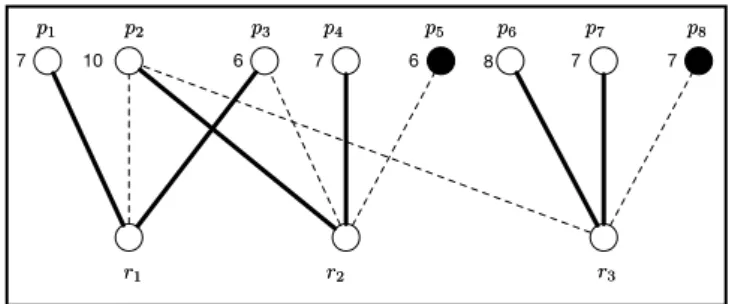
Example 3.1: Let us consider the weighted bipartite graph in Figure 2, whose vertices are the researchers R = {r1, r2, r3} of a universityR and all the publications they have written.
Edges encode the authorship relationproducts, and weights encode the mappingvalproviding the values of the publications. Consider the optimal allocation ψ such thatψ(r1) = {p1, p3}, ψ(r2) = {p2, p4}, andψ(r3) = {p6, p7}, encoded by the solid lines in the figure. Based on
7 10 7 6 8 7 r1 r1 r2r2 r3r3 p2 p2 p3p3 p4p4 p5p5 p6p6 p7p7 7 6 p8 p8 p1 p1
Figure 2.: Authors and products in Example 3.1.
{p1, p2, p3, p4, p6, p7}. The publications that are not submitted are shown in black in the figure.
Note that p2 is co-authored by r1, r2, and r3, while p3 is co-authored by r1 and r2. Thus,
the allocation scenario to be considered isA = hR,Pψ,products,val,2i, and the associated coalitional game is the pair hR,opt(R)i. In particular, the total value of the grand-coalition is
opt(R) = 45.
The problem that we face is how to compute, from the total value obtained byR, a fair score for individual researchers, or groups, or departments, and so on. As mentioned above, product scores are currently used for evaluating the hiring policy of universities and the PhD committees, and starting from 2017 such scores also contribute to evaluate the quality of courses of study. Unfortunately, this is currently done in a way that fails to satisfy the properties that we outline below. Instead, following (Greco & Scarcello, 2013), we propose to use the Shapley value of the allocation game defined by the scenario selected by the given structure R as thedivision rule to distribute the available total value (or budget) to all the participating agents. For the allocation scenario in Example 3.1, we getφr1 =
29
2 ,φr2 = 29
2 , andφr3 = 16. Notice that the
Shapley value is not a percentage assignment of publications to authors, but takes into account all possible coalitions of agents. Note thatr3is not penalized by the fact that its best publication p2 is assigned to researcher r2, in the submission phase determined by the optimal allocation
depicted in Figure 2. Similarly,r1 is not penalized by the fact that the worst publicationp3 is
assigned to her/him (instead of being assigned tor2).
Another important property is that the value assigned to each researcher is independent of the specific selection of products to be submitted, as long as the submission is an optimal one. For instance, an equivalent selection would consist of the products Pψ0 = {p1, p2, p4, p5, p6, p7},
because of the optimal allocation ψ0 such that ψ0(r
1) = {p1, p2}, ψ0(r2) = {p4, p5}, and ψ0(r3) = {p6, p7}. It can be checked that no Shapley value changes for any researcher, by
considering the alternative allocation scenarioA0=hR,P
ψ0,products,val,2ibased on the
se-lection of products Pψ0. On the other hand this nice property does not hold for many division
rules. For instance, assume that the value of each researcher is determined by the average score of all the products evaluated by ANVUR of which he/she is a (co-)author4. Then, in the former allocation scenarior1gets23/3, while in the latter one he/she gets17/2. Symmetrically,r2gets
a higher value in the former scenario and a lower one in the latter.
We will now recall the main desirable properties enjoyed by the division rule based on the Shapley value used in this paper. We refer the interested reader to (Greco & Scarcello, 2013) for a more detailed description and discussion of these properties.
Budget-balance.The division rule precisely distributes the VQR score ofRover all its mem-bers, i.e.,P
r∈Rφr=VR.
Fairness.The division rule is indifferent w.r.t. the specific optimal allocation used to submit the
products to ANVUR. In particular, the score of each researcher is independent of the particular products assigned to him/her in the submission phase; moreover, it is independent of the specific set of productsP selected by the university, as long as the choice is optimal (i.e., with the same maximum valueVR).
Marginality. For any group of researchers S ⊆ R, φS ≥ marg(S,R), where φS =
P
i∈φSφi andmarg(S,R) = opt(R)−opt(R \ S). That is, every group is granted at least
its marginal contribution to the performance of the grand-coalitionR.
We remark the importance of thefairnessproperty, as the choice of a specific optimal set of products is immaterial for R, but it may lead to quite different scores for individuals (and for their aggregations, assume e.g. that researchersr1andr2above belong to different departments).
As a matter of fact, this property does not hold for the division rules adopted by ANVUR for the evaluation of both departments and newly hired researchers (see Section 1.4). The budget-balance property, on the other hand, is violated by the division rule for evaluating researchers who are members of PhD committees.
4. Useful Properties for Dealing with Large Instances
Recall that computing the Shapley value is#P-hard for many classes of games (see, e.g., (Aziz & de Keijzer, 2014; Bachrach & Rosenschein, 2009; Deng & Papadimitriou, 1994; Nagamochi, Zeng, Kabutoya, & Ibaraki, 1997)), including the allocation games, even if goods may have only two possible values (Greco & Scarcello, 2014b).
For large instances, a brute-force approach is unfeasible, because to compute the value of each agenti∈N, it would need to solve2noptimization problems, wheren=|N|is the number of
agents. This is particularly true in our case study, wherenis in the order of thousands.
In order to mitigate the complexity of this problem, in this section we will describe some useful properties of the Shapley value, in particular for allocation problems, which allow us to simplify the instances in a preprocessing phase.
Let us consider in this section an allocation scenarioA=hN,G,Ω,val, ki, withG=hN, vi
denoting its associated game, whose agents graph isG= (N, E). For such scenario we show the following properties which allow us to simplify the game at hand without altering the Shapley value of any player:Modularity,Null goods,Separability,Disconnected agent.
Theorem 4.1(Modularity): Let{C1, C2}be a partition of agents ofN such thatΩ(i)∩Ω(j) = ∅, for every pair of agentsi, jwithi∈C1andj∈C2. LetG1 =hC1, v1i(resp.,G2 =hC2, v2i)
be the coalitional game restricted to agents in C1 (resp., C2). Then, for each agent i ∈ N, φi(G) =φi(G1) +φi(G2).
Proof. LetG01 =hN, v10iandG02 =hN, v02ibe two coalitional games such that, for eachC ⊆N,
v0
1(C) = v1(C∩C1)andv20(C) = v2(C∩C2). Contrasted with the games in the statement,
these games are defined over the full set of agentsN.
Since there are no interactions between agents inC1 and agents inC2, the total value of the
optimal allocation for any coalition C is given by the sum of the values of the goods in the optimal allocations restricted to the two sets of agentsC∩C1andC∩C2. Therefore, we have v(C) =v10(C) +v20(C). Then, from the additivity property of the Shapley value, for each agent
i∈N,φi(G) =φi(G01) +φi(G02).
Consider now the gamesG1 = hC1, v1iandG2 =hC2, v2i) restricted to agents inC1 and in C2, respectively. Note that each playerj ∈ N \C1 isdummywith respect to the gameG01, so
that his/her Shapley value is null, and his/her presence has no actual impact on any other player inG01. In particular such dummy agents could be removed from the game without changing the
Shapley value of the other agents, so that for everyi∈C1, we havesvi(G01) =svi(G1)and the
result immediately follows (by using the same reasoning forG2).
From the above fact, it follows immediately that each connected component of the agents graph can treated as a separate coalitional game.
Corollary 4.2: LetZ be any connected component of the agents graph. The coalitional game
GZ = hZ, vZiassociated with the allocation scenario obtained by restrictingAto the players
inZis such that the Shapley value of each player inZis the same as in the full game associated withA.
It is easy to see that goods having value 0do not impact on the computation of the optimal allocation. However, the existence of shared null goods between multiple agents induces con-nections (among agents) which complicate the structure of the graph.
For instance, consider an allocation scenario A0 comprising three agents{r1, r2, r3} having
a joint interest only for one good, say g0, whose value is0. Any other good has just a single
agent interested in it. In such a scenario, Corollary 4.2 cannot be used, since the agents graph associated with the scenarioA0consists of one connected component. On the other hand, without
g0, the agents graph would be completely disconnected and thus it would be possible to compute
the Shapley values immediately, by using Corollary 4.2. The following fact states that we can indeed get rid of such null goods.
Fact 4.3 (No shared null goods): By removing all goods having value 0 from G, we get an
allocation scenario with the same associated allocation game.
Proof. Just observe that in the computation of the marginal contribution of any agent i to a coalitionC, there is no advantage for agents inCin using a good inΩ(i)having value0.
If it is useful in the algorithms, we can also use Fact 4.3 in the opposite way, and add null-value goods. Letgbe a good withval(g) = 0and letX ={a∈N |g ∈Ω(a)}be the set of agents that are interested in havingg. Then, the game associated withAis the same as the game associated with the allocation scenario wheregis replaced by fresh goodsg1, . . . g|X|such that
each of them is of interest to just one agent inX (hence, there are no connections in the graph because of such goods).
The following property provides us with a powerful simplification method for allocation games. Intuitively, the property states that any set of agents Z that does not exhibit an effec-tive synergy with the rest of the agents can be removed from the game and solved separately.
Theorem 4.4(Separability): LetZbe any coalition such thatopt(Z)+opt(N\Z)≤opt(N). Then, we can define from the allocation scenarioAtwo disjoint allocation scenarios restricted to agents Z and N \Z, respectively, that can be solved separately. For each playeri ∈ N, we can compute its Shapley value in the game associated withAby considering only the game associated with the restricted scenario whereioccurs.
Proof. DenoteN \Z byZ¯, and consider the allocation gamesG1 =hZ, v1iandG2 =hZ, v¯ 2i
restricted to agents inZandZ¯, respectively.
Preliminary observe that, for each pair of disjoint coalitions C0, C00 ⊆ N, opt(C0) +
opt(C00)≥opt(C0∪C00)holds. Indeed, given any optimal allocation for the agents inC0∪C00, its restriction toC0 is a feasible allocation forC0, as well as its restriction toC00 is a feasible
allocation forC00. In particular, we haveopt(Z) +opt( ¯Z) ≥opt(N)that, combined with the hypothesis about the considered coalition Z, entails that opt(Z) +opt( ¯Z) = opt(N). This means that the values of the goods not used in any optimal allocation forZ¯is equal to the sum
of the values of the best goods for the agents inZ.
We shall show that, for each optimal allocationπforN, the set of goodsS ⊆Ω(Z)allocated by π toZ is such thatval(S) = opt(Z)and the analogous property holds for Z¯. Therefore, these agents get the best goods they can obtain. To prove this claim, consider the value v =
val(S)≤opt(Z)and the valuev¯≤opt( ¯Z). We know thatopt(Z) +opt(N \Z) =opt(N)
and, by the optimality ofπ, it holdsv+ ¯v=opt(N)too.
Consider now any coalitionC ⊆N, and letCa=C∩ZandCb =C∩Z¯. Letπ0be an optimal
allocation for C. We claim that there is an optimal allocationπamapping goods from S toZ
withvalπa(Ca) = valπ0(Ca), and an optimal allocationπb mapping goods not inS toZ¯with
valπb(Cb) =valπ0(Cb). Assume by contradiction that this is not the case. Then at least one of those allocations leads to values smaller than those inπ0(note thatπ0 cannot be worse, because the union of the two restricted allocations is a valid candidate mapping forC). AssumeCagets
a smaller total value (the other case is symmetrical), that is, valπa(Ca) < valπ0(Ca). Then, there exists some agentiand a goodp /∈S so thatp ∈π0(i). By using Theorem 4.4 in (Greco
& Scarcello, 2014b), we can show that this would contradict the fact that val(S) = opt(Z). In fact, goods such aspthat are shared with agents outsideZ and that allows us to get a better value for the agents inCa ⊆ Z, could be used to improve the choice of the available goodsS
for the full setZ.
Now, given that it suffices to use only the goods inS for Z and the remaining goods forZ¯, we can define an equivalent game in which the goods inSare of interest to agents inZonly and the remaining to agents inZ¯ only. In the new game,Z andZ¯ are in fact sets of agents with no shared connections and the theorem follows immediately from Theorem 4.1.
A very frequent and important case in applications, which falls in the case considered by this latter property, occurs whenCis a singleton{i}, and it happens that the optimal allocation for this coalition is equal to the marginal contribution ofitoN\{i}. By using the property described above, the set ican be removed from the game and solved separately, so that we immediately getφ(i) =opt({i}).
The following property identifies some goods that are useless for some agentiand thus can be safely removed from its set of relevant goodsΩ(i). Note that this operation does not affect other agents possibly interested in such goods.
Fact 4.5 (Useless goods): Let i ∈ N be an agent, and let g ∈ Ω(i) be a good such that
val(g) + maxg0∈Ω(i)\{g}val(g0)<margi(N). Then, the modified allocation scenario whereg
is removed fromΩ(i)is equivalent to the original one, that is, the two scenarios have the same associated game.
We conclude this section with a simple property that does not help to simplify the game, but allows us to avoid the computation of unnecessary optimal allocations, during the computation of marginal contributions.
Fact 4.6 (Disconnected agent): Leti ∈ N be an agent and letC ⊆ N be a component dis-connected fromi, that is, such thatΩ(i)∩Ω(j) = ∅, for eachj ∈ C. Then,opt({i} ∪C) =
opt({i}) +opt(C)holds and the marginal contribution ofitoCisopt({i}).
5. Lower and Upper Bounds for the Shapley Value
In this section we describe the computation of a lower bound and an upper bound for the Shapley value of the allocation gameGA =hN, vAiassociated with any given allocation scenarioA=
The availability of such bounds can be helpful to provide a more accurate estimation of the approximation error in randomized algorithms. Moreover, whenever the two bounds coincide for some agent, we clearly get the precise Shapley value for that agent. We shall see that this often occurs in practice, in our case study.
Preliminarily observe that in allocation games we have for free a simple pair of bounds from the anti-monotonicity property of these games: for each pair of coalitions C1 ⊆ C2,
margi(C2) ≤ margi(C1). Then, for each playeri and for every coalitionC ⊆ N \ {i}, we
havemargi(N)≤margi(C)≤margi(∅) =opt({i}). It immediately follows that
margi(N)≤φi≤opt({i}).
P' i Z LB UB P' i Z (a) (b) P' i Z P' i Z (c) (d)
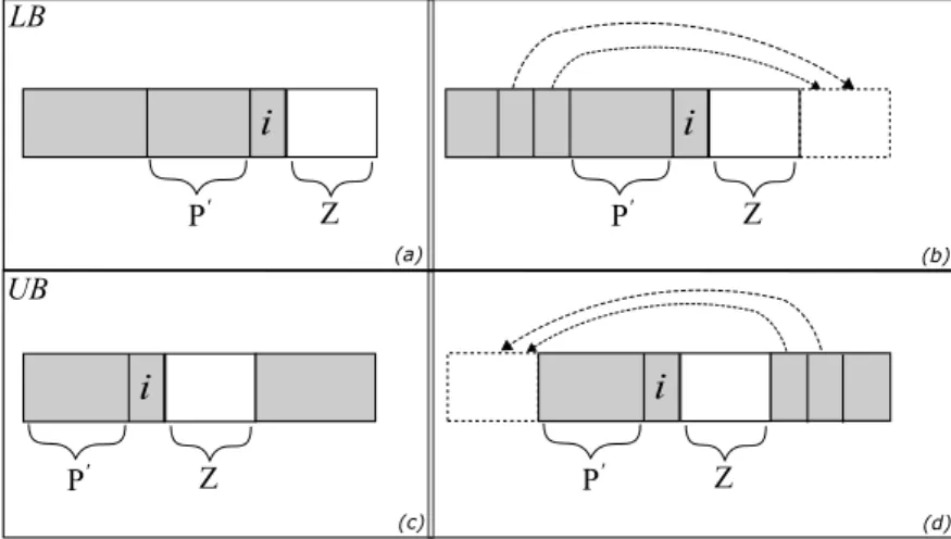
Figure 3.: Neighborhood configurations
In order to obtain tighter bounds, we observe that, given any coalitionCand an agenti /∈C, the neighbors ofiin the agents graph that belong toChave the higher influence on the marginal contribution ofitoC. Indeed, they are precisely those agents interested in using the goods ofi
when he/she does not belong to the coalition. We already observed that, in the extreme case that no neighbors are present,icontributes with all his/her best goods. The idea is to consider the power-set ofNeigh(i)as the only relevant sets of agents.
LetP0be a set of neighbors ofi, letZ =Neigh(i)\P0, and letC =N\(Neigh(i)∪ {i}). For the computation of the lower bound in Algorithm 1, for such a profileP0 we compute the marginal contribution of itoC∪P0 (see Figure 3.a), but use this same value for the marginal contributions of ito every coalition C0 ⊆ N such thatC0∩Neigh(i) = P0, that is, for every
coalition with the same configuration P0 of neighbors ofi(Figure 3.b). Furthermore, we use a suitable factoryto weigh this value in order to simulate that every such a coalitionC0 gets that
same marginal contribution fromi.
The case of the upper bound is obtained in the dual way, by using instead the most favorable case, i.e., by using the marginal contribution of ito P0 (Figure 3.c) in place of the marginal contribution ofito any coalitionC0 ⊆N withC0∩Neigh(i) =P0(Figure 3.d).
Theorem 5.1: Let (LB, U B) be the output of Algorithm 1. For each agent i ∈ N, LBi ≤
φ(i)≤U Biholds, and the computation of such values can be done in timeO(2|Neigh(i)||N|3).
Proof. Letibe an agent of the game. As discussed above and depicted in Figure 3, the algorithm is based on the computation of any possible combinationP0of the neighbors ofi. Regarding the computation of the lower bound, for each such profile P0, the algorithm considers a coalition
Algorithm 1Computing Bounds for the Shapley Value in Allocation Games
Input:An allocation gameGA=hN, vAi;
Output:A pair of vectors(LB, U B)encoding, respectively, a lower bound and an upper bound of the Shapley value ofGA;
1: for alli∈N do 2: P :=P owerset(Neigh(i)); 3: C :=N \(Neigh(i)∪ {i}); 4: l=|C|; 5: for allP0 ∈P do 6: Z :=Neigh(i)\P0; 7: y=Plk=0 (l−k+|P 0|)!·(|Z|+k)! |N|! · l k ; 8: LBi +=y·(vA(C∪P0∪ {i})−vA(C∪P0)); 9: U Bi +=y·(vA(P0∪ {i})−vA(P0)); 10: end for 11: end for 12: return(LB, U B);
C∪P0 obtained by completingP0with all the agents inN \ {i}that are not neighbors ofi.
The algorithm uses the value of the marginal contribution of ito such coalition, that is, the valuemargi(C∪P0) =vA(C∪P0∪ {i})−vA(C∪P0), in place of the marginal contributions
ofito each coalitionC0 ⊆N such thatC0∩Neigh(i) =P0. Now, becauseC0 ⊆C, by the anti-monotonicity property of the marginal contributions in allocation games, we havemargi(C)≤
margi(C0). Then, the algorithm weighs in a suitable waymargi(C ∪P0) so that it is used in place of the right marginal contribution ofito each coalitionC0of the form described above. A simple combinatorial argument shows that this can be achieved by multiplyingmargi(C∪P0)
by the following factor
y= l X k=0 (l−k+|P0|)!·(|Z|+k)! |N|! · l k , (1)
wherel=|N \(Neigh(i)∪ {i})|andZ =Neigh(i)\P0.
Regarding the computation of the upper bound of the Shapley value ofi, we proceed in a sim-ilar way, but using the marginal contribution ofito the profileP0 containing only its neighbors, instead of the marginal contributions to the various coalitionsC0 ⊆N such thatC0∩Neigh(i) =
P0. Indeed, in this case we haveP0 ⊆C0and thereforemargi(C0)≤margi(P0). Again, we need to multiply such value by a factor which takes into account all possible ways of extendingP0to any coalitionC0with the same profile ofi’s neighbors. It is easy to see that we can again use the factorydescribed above, by exploiting the fact that kl= l−lk.
Concerning the computational complexity, just observe that, for each elementP0of the power set of Neigh(i), we have to solve a constant number of optimal allocation problems. Each of these problems requires the computation of an optimal weighted matching, which can be solved in timeO(|N|3).
6. Approximating the Shapley Value
6.1. A Fully Polynomial-time Randomized Approximation Scheme
Recall that a coalitional gameG= (N, v)issupermodular(Shapley, 1971) if
v(S∪ {i})−v(S)≤v(T∪ {i})−v(T), wheneverS⊆T andi /∈T;
in other words, the marginal contribution of playerito coalitionSis not greater thani’s marginal contribution to any larger coalition T ⊇ S. Moreover, it is said monotoneif v(C) ≤ v(C0)
wheneverC⊆C0.
Supermodular games have nice computational properties (see, e.g., Maschler, Peleg, & Shap-ley, 1971; Kannai, 1992; Hatano & Yoshida, 2017). In particular, Liben-Nowell et al. (2012) have shown that they have a Fully Polynomial-time Randomized Approximation Scheme (FPRAS): for any > 0andδ > 0, it is possible to compute in polynomial-time an−approximation of the Shapley value of a monotone supermodular game with probability of failure at mostδ.
Note that allocation games are not supermodular, however Greco and Scarcello (2014b) proved that, for each allocation gameG, there is a monotone supermodular game that is equiva-lent toGwith respect to the computation of the Shapley value. In particular, from the definition of this equivalent game, it is straightforward to see that one can apply the FPRAS algorithm to either game, obtaining the same approximation guarantees.
Recall that the FPRAS method by Liben-Nowell et al. (2012) is based on generating a certain number of permutations (of all agents) and computing the marginal contribution of each agent to the coalition of agents occurring before him/her in the considered permutation. Then the Shapley value of each player is computed as the average of all such marginal contributions. The above procedure is repeated O(log(1/δ)) times, in independent runs, with the result for each agent consisting of the median of all computed values for him/her. Finally, the obtained values are scaled (i.e., they are all multiplied by a common numerical factor) to ensure that the budget-balance property is not violated.
Clearly enough, the more permutations are considered, the closer to the Shapley value the result will be. We next report a slightly modified version of the basic procedure of this algorithm, where we avoid the computation of some marginal contributions, if we can obtain the result by using Fact 4.6.
As a preliminary step, we compute the required number of permutations m to meet the re-quired error guarantee. In each of themiterations, the algorithm generates a random permuta-tion from the set of agentsN. We then iterate through this permutation and compute the marginal contribution of each agentjto the set of agentsCoccurring beforejin the permutation at hand. If some neighbor ofj(in the agents graph) occurs inC, the algorithm proceeds as usual by com-puting the value of an optimal allocation forC∪ {j}in order to obtain the valuevA(C∪ {j}). Note that this one computation is indeed sufficient to get such a marginal contribution, because the valueopt(C)for the coalitionCincluding the preceding agents (for the permutation at hand) is known from the previous step. Moreover, by Fact 4.6, we know that for those permutations in which all the players in Neigh(j)followj, the marginal contribution ofj is just opt({j})
(see step 10). Finally, at steps 16–18 for each agent the algorithm divides the sum of his/her contributions by the number of performed iterationsm. The correctness of the whole algorithm follows from Theorem 4 in (Liben-Nowell et al., 2012).
Computation Time Analysis. Letn = |N|be the number of agents, and letmbe the required number of iterations. The cost of the algorithm isO(m×n×margBlock), wheremargBlock
denotes the cost of computing each marginal contribution (steps 7–11). This requires the com-putation of an optimal weighted matching in a bipartite graph, which is feasible inO(n3), via
Algorithm 2Shapley value approximation in allocation games
Input:An allocation gameGA=hN, vAi;
Parameters:Real numbers0< <1and0< δ <1;
Output: A vector φ˜ that is an-approximation of the Shapley value ofGA, with probability 1−δ; 1: m= |N|·(δ|·N2|−1); 2: i= 0; 3: whilei < mdo 4: shuffle(N); 5: C :={∅}; 6: for allj∈N do 7: ifNeigh(j)∩C 6=∅then 8: φ˜j +=vA(C∪ {j})−vA(C); 9: else 10: φ˜j +=vA({j}); 11: end if 12: C:=C∪ {j}; 13: i=i+ 1; 14: end for 15: end while 16: for allj∈N do 17: φ˜j = ˜ φj m; 18: end for 19: returnφ˜;
the classical Hungarian algorithm(Kuhn & Yaw, 1955). However, if the current agent is dis-connected from the rest of the coalition, the cost is given by a simple lookup in the cache where the best allocation for each single agent is stored.
6.2. Sampling Algorithm When the Range of Marginal Contributions Is Known
Maleki et al. (2013) propose a bound on the number of samples (over the population of marginal contributions) required to estimate an agent’s Shapley value, when the range of his/her contribu-tions is known. Their bound is based on Hoeffding’s inequality (Hoeffding, 1963), and it states that, in order to approximate the Shapley value of agentiwithin an absolute value, with failure probability at mostδi, that is, in order to get
P rob{|φ˜i−φi| ≥} ≤δi (2)
at leastmisamples are required, where:
mi= & ln (δ2 i)·r 2 i 2·2 ' (3)
In the above expression,ridenotes the range ofi’s marginal contributions (i.e.,ri =opt({i})−
bound allows us to determine the number of required random samples for each agenti, once
and δi are fixed. Assuming we want an overall failure probability δ, each agent i ∈ N could
be assigned a failure probabilityδi = δ/|N|. In principle a higher failure probabilityδi could
be tolerated for agents with larger ranges, at the expense of lower failure probability for agents with smaller ranges. However, our experimental tests performed with this variant exhibited only a few marginal gains.
Once the number of required samples for each agent is determined, the approximate Shapley value, with the desired guarantees on the absolute error, can easily be computed by a randomized algorithm evaluating the required samples of coalitions for each player (see Section 7.1 for a brief description of our parallel implementation).
In order to consider the classical percentage expression for the approximation error, we should replace by ·φi in (2). First observe that φi 6= 0for all agents ithat are considered by the
algorithm, because our simplification techniques preliminarily identify and remove from the game those agents having a null Shapley value (these agents must be interested only in goods with a null value). In fact, the value of φi that would appear in (3) may be replaced by any
known (non-null) lower bound`i ≤φi, at the expense of taking more samples than those strictly
necessary. On our largest test instance (namely, the researchers of Sapienza University of Rome who participated in the research assessment exercise VQR2011-2014), the technique described in Section 5 yields lower bounds that are greater that0for all agents. It turns out that, in a matter of hours, we are able to get approximate Shapley values within5%of the correct values.
It should be noted that the bound presented by Maleki et al. (2013), due to the exponential relation it establishes between mi and δi, allowed us to compute good approximate Shapley
values at least for our test instances, where the range of the marginal contributions is fairly limited, in a matter of hours. As a comparison, the FPRAS approach described in Section 6.1 would have taken a few years, instead of a few hours, to process our largest input instance with the same error guarantees (see Section 7 for details on our experiments).
7. Implementation Details and Experimental Evaluation 7.1. Parallel Implementation of Shapley Value Algorithms
All the algorithms considered in this paper are amenable to parallel implementation. We engi-neered our parallel implementations as follows.
FPRAS algorithm (Liben-Nowell et al., 2012). Besides the input allocation game, and the two parametersδand, we added a third parameter, thethread pool size. During the execution of the algorithm, each thread (there are as many threads as the thread pool size dictates) is responsible for generating a certain number of permutations according to the requested approximation factor and, for each permutation, it computes the marginal contributions of all authors to that permu-tation, and saves them in a local cache. Whenever a thread has generated its assigned number of permutations, it delivers its local cache of computed scores to a synchronized output acceptor (which increments the overall score of each author accordingly), and then shuts itself down as its work is completed. When all threads have shut down, each entry of the acceptor’s output vector is averaged over the total number of permutations, yielding the final approximate Shapley vector for that run. The above procedure is repeated for each independent run. When all runs are done, the component-wise median of all final approximate Shapley vectors is computed, and the re-sulting vector is scaled (i.e., all entries are multiplied by a number such that the budget-balance property is enforced), yielding the desired approximation with the desired probability.
number of required samples for each author i is determined by a sequential routine (as this computation is very fast), based on the approximation parametersδand, and on precomputed values foropt({i}),marg({i}, N), whereN is the set of all authors, andLBi. The algorithm
also receives two extra parameters,threadP oolSizeandbatchSize. Subsequently, each thread (the total number of threads is determined bythreadP oolSize) asks a synchronized producer for a job (i.e., a pair (i, numSamples)). The synchronized producer either provides a job for the requesting thread, or it returns null, if enough jobs have already been distributed to sat-isfy the approximation requirements. Upon receiving a job, a thread produces numSamples
uniformely distributed random subsets of N \ {i}, and for each such subset S, computes the marginal contribution of itoS. The sum of these contributions is delivered to a synchronized output acceptor, which stores, for each author, the sum of all marginal contributions computed so far by the various threads. Notice that the job provider will always distribute pairs for which
numSamples≤batchSize. This is done to ensure, with proper tuning of parameterbatchSize, load balancing between the threads. Finally, when a thread receivesnullfrom the synchronized job provider, it simply shuts itself down, as there is no more work to do. When all threads have shut down, the output acceptor will average the sum of all marginal contributions of each author over the number of required samples for that author, yielding the approximate Shapley value. Exact algorithm.In our exact algorithm implementation, each thread (the total number of threads is specified by an input parameter) asks a synchronized producer for a subset of authors to work with. The synchronized subset producer either provides ann-bit integer number (wherenis the number of authors) for the requesting thread, or it returnsnullif all2nsubsets have already been delivered for elaboration. Upon receiving an n-bit integer from the subset provider, a thread turns it into a subset of authors (if a bit is set to 1, then the corresponding author is included in the subset), and computes partial scores for all authors in the subset, storing the values obtained in a local cache. When a thread receivesnullfrom the subset provider, it delivers its local cache of computed scores to a synchronized output acceptor (which increments the overall score of each author accordingly), and then shuts itself down, as it has no more work to do. When all threads have shut down, the output vector will contain the exact Shapley values for all authors.
7.2. Experimental Results
Hardware and software configuration.Experiments have been performed on two dedicated ma-chines. In particular, sequential implementations were run on a machine with an Intel Core i7-3770k 3.5 GHz processor, 12 GB (DDR3 1600 MHz) of RAM, and operating system Linux Debian Jessie. We tested the parallel implementations on a machine equipped with two Intel Xeon E5-4610 v2 @ 2.30GHz with 8 cores and 16 logical processors each, for a total of 32 logi-cal processors, 128 GB of RAM, and operating system Linux Debian Wheezy. Algorithms were implemented in Java, and the code was executed on the JDK 1.8.0 05-b13, for the Intel Core i7 machine, and on the OpenJDK Runtime Environment (IcedTea 2.6.7) (7u111-2.6.7-1 deb7u1), for the Intel Xeon machine.
Dataset description.We applied the algorithms to the computation of a fair division of the scores for the researchers of Sapienza University of Rome who participated in the research assessment exercise VQR2011-2014. Sapienza contributors to the exercise were 3562 and almost all of them were required to submit 2 publications for review. We computed the scores of each publication by applying, when available, the bibliographic assessment tables provided by ANVUR.
Preprocessing. The analysis was carried out by preliminarily simplifying the input using the properties discussed in Section 4, as explained next.
a10 a4 a3 a1 a11 a13 a14 a6 a7 a2 a8 a9 a12 a0 a5 Agents 0 10 20 30 40 50 60 70 80 90 100 110 120 130 140 150 160 170 180 190 200 210 V alues LB FPRAS Maleki et al. Exact UB
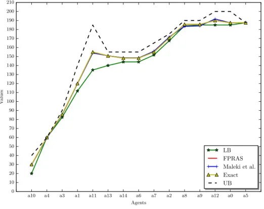
Figure 4.: Methods comparison (n= 15).
researchers having no publications for review. After this step a total of 370 authors were re-moved. Then, by exploiting the simplification described in Fact 4.3, we removed 2323 publica-tions. By using Theorem 4.4, the graph was subsequently filtered removing each author whose marginal contribution to the grand coalition coincided with the optimal allocation restricted to the author himself. After this step 2427 researchers out of 3562 were removed. Then we divided the resulting agents graph into connected components obtaining a total number of 156 con-nected components and we discovered only two components consisting of more than 10 agents. The sizes of these components were 691 and 15. These components were further simplified by using Fact 4.5. After the whole preprocessing phase, we obtained a total of 159 connected com-ponents with the largest one having 685 nodes. The size of the second largest component was 15, while all the others remained very small (less than 10 nodes). In the rest of the section, we shall illustrate results of experimental activity conducted over the various methods. To this end, we fix the valueδ= 0.01. This value has been chosen heuristically, based on a series of tests conducted on various CUN Areas of Sapienza, where CUN Areas are (large) scientific disciplines such as Math and Computer Science (Area 01) or Physics (Area 02).
Tests with components of variable size.As already pointed out, after the preprocessing step we obtained very small connected components (less than 10 nodes) except for the largest two (685 and 15 nodes, respectively). For all components with less than 10 nodes, the exact algorithm, of which we used a sequential implementation for these tests, performs very well (a few millisec-onds), therefore we omit the analysis here. In order to test all the other algorithms, besides the two largest components, we randomly extracted samples of (distinct) nodes out of the original graph, to produce different subgraphs with sizen∈ {23,26,30,40}.
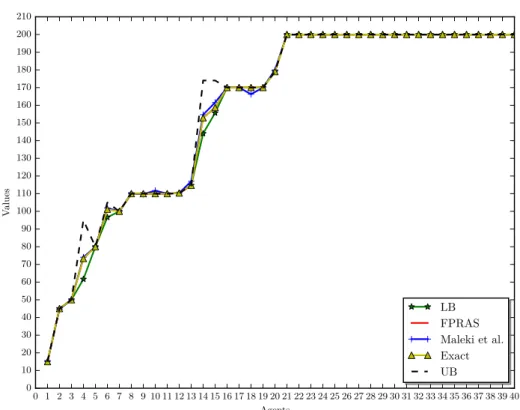
For the considered cases, we do not find significant differences among the values obtained by using the two approximation algorithms and the exact ones (see, e.g., figures 4 and 5, in which
0 1 2 3 4 5 6 7 8 9 10 11 12 13 14 15 16 17 18 19 20 21 22 23 24 25 26 27 28 29 30 31 32 33 34 35 36 37 38 39 40 Agents 0 10 20 30 40 50 60 70 80 90 100 110 120 130 140 150 160 170 180 190 200 210 V alues LB FPRAS Maleki et al. Exact UB
Figure 5.: Methods comparison (n= 40).
the approximation algorithms were required to produce results within 5% of the exact value5). Notably, with the exception of a small number of cases, our bounds (especially the lower bounds) are always very close to the exact value. In particular, forn= 26we were able to immediately get the Shapley value for all agents, since upper and lower bounds coincide for all of them.
We also evaluated how many computations of optimal allocations were avoided in the FPRAS of Liben-Nowell et al., by exploiting Fact 4.6 (and hence executing in the latter case Step 10 rather than Step 8 in Algorithm 2). By fixing the approximation error at = 0.3, for each
n ∈ {15,23,26,30,40} we get the following savings: 9.65·105 out of 3.5·106 (i.e., 28%),
2.34·106out of1.29·107(18%),5.36·106out of1.87·107 (29%),8.78·106 out of2.9·107
(30%), and1.46·107out of6.93·107 (21%), respectively.
As already pointed out, the FPRAS method performed much better than its theoretical guaran-tee on the maximum approximation error. We report the real maximum and average approxima-tion errors (denoted by X and Y, respectively) of our implementaapproxima-tion w.r.t. the exact algorithm for each n ∈ {15,23,26}, with = 0.3. Forn = 15, we get X = 0.01 and Y =3·10−3, for
n= 23we get X =1.5·10−3and Y =1.7·10−4, and forn= 26we get X =1.06·10−4and Y
=1.59·10−5. In all cases, the maximum approximation error was about 1% (or less) and there-fore considerably below the theoretical guarantee (30%). The algorithm based on the bound of Maleki et al. also performs better than its theoretical guarantee, though not by as wide a margin as the FPRAS method (it is, however, much faster, as we will see in the next paragraph). In this case, forn= 15we get X = 0.093 and Y = 0.046, forn= 23we get X = 0.098 and Y = 0.011, and forn= 26we get X = 0.097 and Y = 0.019. In all cases, the maximum approximation error was below 10%, and therefore quite smaller than the required threshold.
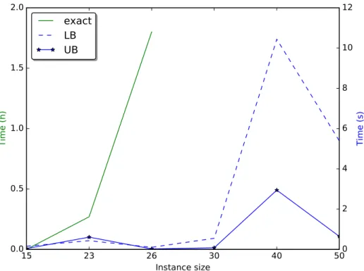
Running Times.Figures 6, 7 and 8 report the computation times of the various algorithms. In
15
23
26
30
40
50
Instance size
0.0
0.5
1.0
1.5
2.0
Time (h)
exact
LB
UB
0
2
4
6
8
10
12
Time (s)
Figure 6.: Sequential implementations: running times for the computation of the exact value by using the brute-force algorithm (green), and of the upper and lower bounds (blue) vs instance size.
particular, Figure 6 focuses on the sequential implementations of the brute-force algorithm for computing the exact values, and of the algorithms for computing the upper and lower bounds. For the experiments, we computed separately the two bounds in order to point out that the computation of the lower bound requires in general more time, because it considers allocation over larger coalitions than those considered for the computation of the upper bound. Moreover, as discussed in Section 5, the running times for computing the bounds heavily depend on the cardinality of the agents’ neighborhoods. This explains why the running times for the casen= 50are smaller than those for the casen= 40.
Figure 7 shows the running time of the parallel implementation of the FPRAS method, us-ing 24 threads, for different values of. In particular, we performed five trials over the different (sub)games described above, and report averaged measures. We can see that for games of reason-able size we can achieve a high theoretical approximation error guarantee. For instance, for the largest considered game (n= 50) we were able to compute the approximate Shapley value with
= 0.1in less than 90 minutes. There is a wide gap between the running times of the FPRAS method, when using the highest and lowest values we considered for the allowed approximation error. However, as already pointed out, even when we used a poor theoretical guarantee on the approximation error, we still obtained a quite reasonable accuracy.
In spite of its excellent accuracy, and its high efficiency when compared to the exact algorithm, we estimated that our parallel implementation of the FPRAS method would have taken, with= 0.05and 24 threads, roughly3.33years to fully analyze the largest component of our Sapienza test case, comprising 685authors. By contrast, the parallel implementation of the algorithm based on the bound proposed by Maleki et al., with the same settings, took only 11.75 hours. The bound on the number of samples proposed by Maleki et al. requires the knowledge of the range of the marginal contributions, which was computed in less than 3 minutes. Moreover,
90 80 70 60 50 40 30 20 10 5 Maximum allowable MC error (%)
0 20 40 60 80 Time (min) 89.12 min 1.08 min 37.82 min 1.64 min 8.53 min 0.41 min 4.60 min 0.25 min 3.74 min 0.21 min 0.41 min 0.06 min n=50 n=40 n=30 n=26 n=23 n=15
Figure 7.: Parallel implementation of FPRAS method: running times vs.
90 80 70 60 50 40 30 20 10 5 1 Absolute Error 0 200 400 600 800 1000 1200 Time (min) 338.00 min 3.61 min 1226.31 min 12.85 min n=685 n=1176
Figure 8.: Parallel implementation of Maleki-based algorithm: running times vsabs.
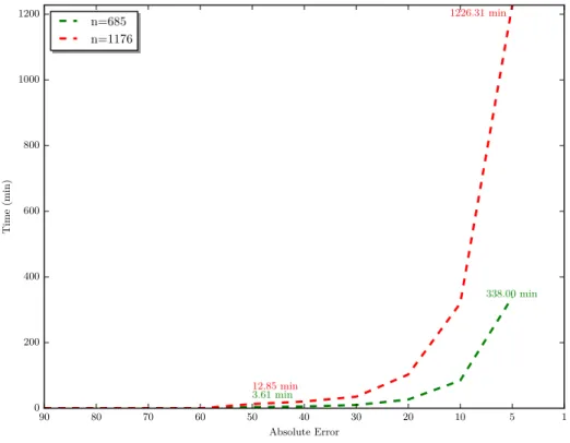
lower bounds for the Shapley value are also required. For the largest component of our test instance, we computed the lower bounds for the 681 authors with neighborhood size up to 19; for the few remaining authors with more neighbors (just 4 authors), we used as lower bound the marginal contribution to the grand coalition. Multithreaded computation of the lower bounds took approximately 160 hours.
It should be noted that the bound by Maleki et al. can also be applied directly to the largest CC in the unsimplified Sapienza VQR graph. This CC comprises 1176 authors. In this case, straight-forward application of the bound for all authors required, on our server, with 24 threads and an absolute errorabs = 5, roughly 20.5 hours. If we setabs = 1, the computation time increases
to approximately 31 days. Figure 8 shows the running times of the parallel implementation of Maleki-based algorithm on the two largest CCs in our test instances, with varying values ofabs.
8. Conclusions and Future Work
In this paper, we have identified useful properties that allow us to decompose large instances of allocation problems into smaller and simpler ones, in order to be able to compute the Shapley value. The proposed techniques greatly improve the applicability to real-world problems of the approximation algorithms described in the literature. Furthermore, we described an algorithm for the computation of an upper bound and a lower bound for the Shapley value. These bounds provide a more accurate estimate of approximation errors, and (often, in our case study) yield the exact Shapley value for those agents where upper and lower bounds coincide.
We have engineered parallel implementations of the considered algorithms, and we have tested them on a real-world problem, namely, the 2011-2014 Italian research assessment program (known as VQR), modeled as an allocation game. With the proposed tools, we have been able to compute, either exactly, or within a fairly good approximation (5% of the correct value with 99% probability) the Shapley value for all agents in our largest test instance, namely, Sapienza University of Rome, comprising 3562 researchers and 5909 research products.
As future work, we would like to extend the structure-based technique described in (Greco et al., 2015) to the more general class of games where more than one good can be allocated to each agent (as it is the case in VQR allocations). In this way, we could compute efficiently the exact Shapley value for large games, provided that the treewidth of the agents graph is small. With this respect, we note that this is not the case for the large Sapienza VQR instance for which, after the simplification performed with the tools described in the paper, we are left with a large component whose estimated treewidth is 64. This is too much for using structure-based decomposition techniques. However, for the sake of completeness, we note that all other components have a low treewidth. For instance, the component with 50 agents used in our tests has treewidth 5.
Finally, we would like to obtain tighter lower and upper bounds, possibly with a computational effort that can be tuned to meet given time constraints.
References
Aziz, H., & de Keijzer, B. (2014). Shapley meets shapley. In31st international symposium on theoretical aspects of computer science (STACS 2014), STACS 2014, march 5-8, 2014, lyon, france(pp. 99– 111). Retrieved fromhttp://dx.doi.org/10.4230/LIPIcs.STACS.2014.99 Bachrach, Y., & Rosenschein, J. S. (2009, February). Power in threshold network flow games.
Au-tonomous Agents and Multi-Agent Systems,18(1), 106–132. Retrieved fromhttp://dx.doi .org/10.1007/s10458-008-9057-6
Castro, J., G´omez, D., & Tejada, J. (2009, May). Polynomial calculation of the shapley value based on sampling. Comput. Oper. Res.,36(5), 1726–1730. Retrieved fromhttp://dx.doi.org/
10.1016/j.cor.2008.04.004 doi:
Deng, X., & Papadimitriou, C. H. (1994, May). On the complexity of cooperative solution concepts.
Mathematics of Operations Research,19, 257–266. Retrieved from http://dl.acm.org/ citation.cfm?id=183315.183317
Greco, G., Lupia, F., & Scarcello, F. (2015). Structural tractability of shapley and banzhaf values in allocation games. InProceedings of the twenty-fourth international joint conference on artificial intelligence, IJCAI 2015, buenos aires, argentina, july 25-31, 2015(pp. 547–553). Retrieved from http://ijcai.org/papers15/Abstracts/IJCAI15-083.html
Greco, G., & Scarcello, F. (2013). Fair division rules for funds distribution: The case of the italian research assessment program (vqr 2004-2010). Intelligenza Artificiale, 7(1), 45–56. Retrieved from http://content.iospress.com/articles/intelligenza -artificiale/ia042
Greco, G., & Scarcello, F. (2014a). Counting solutions to conjunctive queries: structural and hybrid tractability. In Proceedings of the 33rd acm sigmod-sigact-sigart symposium on principles of database systems, pods’14, snowbird, ut, usa, june 22-27, 2014(pp. 132–143). Retrieved from http://doi.acm.org/10.1145/2594538.2594559
Greco, G., & Scarcello, F. (2014b). Mechanisms for fair allocation problems: No-punishment payment rules in verifiable settings. J. Artif. Intell. Res. (JAIR),49, 403–449. Retrieved fromhttp:// dx.doi.org/10.1613/jair.4224
Hatano, D., & Yoshida, Y. (2017). Computing least cores of supermodular cooperative games. In S. P. Singh & S. Markovitch (Eds.), Proceedings of the thirty-first AAAI conference on arti-ficial intelligence, february 4-9, 2017, san francisco, california, USA. (pp. 551–557). AAAI Press. Retrieved from http://aaai.org/ocs/index.php/AAAI/AAAI17/paper/ view/14607
Hoeffding, W. (1963). Probability inequalities for sums of bounded random variables. Journal of the American Statistical Association,58(301), 13-30. Retrieved fromhttp://www.tandfonline .com/doi/abs/10.1080/01621459.1963.10500830
Iera, A., Militano, L., Romeo, L., & Scarcello, F. (2011). Fair Cost Allocation in Cellular-Bluetooth Cooperation Scenarios. IEEE Transactions on Wireless Communications,10(8), 2566–2576. Kannai, Y. (1992). The core and balancedness. Handbook of game theory with economic applications,1,
355–395.
Kuhn, H. W., & Yaw, B. (1955). The hungarian method for the assignment problem. Naval Res. Logist. Quart, 83–97.
Liben-Nowell, D., Sharp, A., Wexler, T., & Woods, K. (2012). Computing shapley value in supermod-ular coalitional games. In J. Gudmundsson, J. Mestre, & T. Viglas (Eds.),Computing and com-binatorics: 18th annual international conference, cocoon 2012, sydney, australia, august 20-22, 2012. proceedings(pp. 568–579). Berlin, Heidelberg: Springer Berlin Heidelberg. Retrieved from http://dx.doi.org/10.1007/978-3-642-32241-9 48
Lupia, F., Mendicelli, A., Ribichini, A., Scarcello, F., & Schaerf, M. (2016). Computing the shapley value in allocation problems: Approximations and bounds, with an application to the italian VQR research assessment program. InProceedings of the 23rd RCRA International Workshop on Ex-perimental Evaluation of Algorithms for Solving Problems with Combinatorial Explosion 2016 (RCRA 2016) A workshop of the XV International Conference of the Italian Association for Arti-ficial Intelligence (AI*IA 2016), Genova, Italy, November 28, 2016.(pp. 27–43). Retrieved from http://ceur-ws.org/Vol-1745/paper3.pdf
Maleki, S., Tran-Thanh, L., Hines, G., Rahwan, T., & Rogers, A. (2013). Bounding the estimation error of sampling-based shapley value approximation with/without stratifying. CoRR,abs/1306.4265. Retrieved fromhttp://arxiv.org/abs/1306.4265
Maniquet, F. (2003). A characterization of the Shapley value in queueing problems.Journal of Economic
Theory,109(1), 90-103. Retrieved fromhttp://www.sciencedirect.com/science/
Maschler, M., Peleg, B., & Shapley, L. S. (1971). The kernel and bargaining set for convex games.
International Journal of Game Theory,1(1), 73–93.
Mishra, D., & Rangarajan, B. (2007, October). Cost sharing in a job scheduling problem. Social Choice and Welfare,29(3), 369-382. Retrieved fromhttp://ideas.repec.org/a/spr/ sochwe/v29y2007i3p369-382.html
Moulin, H. (1992, November). An application of the Shapley value to fair division with money.
Econo-metrica, 60(6), 1331-49. Retrieved from http://ideas.repec.org/a/ecm/emetrp/
v60y1992i6p1331-49.html
Nagamochi, H., Zeng, D.-Z., Kabutoya, N., & Ibaraki, T. (1997, February). Complexity of the mini-mum base game on matroids. Mathematics of Operations Research,22, 146–164. Retrieved from http://dl.acm.org/citation.cfm?id=265654.265660
Osborne, M. J., & Rubinstein, A. (1994). A course in game theory. Cambridge, MA, USA: The MIT Press.
Robertson, N., & Seymour, P. (1984, February). Graph minors iii: Planar tree-width. Journal of Combi-natorial Theory, Series B,36(1), 49–64.
Shapley, L. S. (1953). A value for n-person games. Contributions to the theory of games,2, 307–317. Shapley, L. S. (1971, Dec 01). Cores of convex games. International Journal of Game Theory,1(1),
11–26. Retrieved fromhttps://doi.org/10.1007/BF01753431 doi:
Stein, C. (1972). A bound for the error in the normal approximation to the distribution of a sum of dependent random variables. In Proceedings of the sixth berkeley symposium on mathematical statistics and probability, volume 2: Probability theory(pp. 583–602). Berkeley, Calif.: Univer-sity of California Press. Retrieved fromhttps://projecteuclid.org/euclid.bsmsp/ 1200514239