Software Defect Prediction Using Static Code Metrics: Formulating a Methodology

(1)

Software Defect Prediction

Using Static Code Metrics :

Formulating a Methodology

David Philip Harry

_Gray

December 2012

Submitted to the University of Hertfordshire in partial

fulfilment of the requirements of the degree of

Doctor of Philosophy

(2)

(3)

Acknowledgements

First and foremost, I would like to thank my parents. Thank you for an amazing upbringing, for constant love and support, and for the wisdom I have learnt from you both. Without your support in so many aspects of my life, I would never have reached where I am today. Just think, if only you had chosen to stick to the original plan of naming me Philip Harry David Gray, I could of had two PhD’s to my name! However, I’m proud to be DPHG PhD, I hope you’re proud too.

I would now like to thank my supervisors. Firstly, to David Bowes, for believing in me. Had it not been for your advice and encouragement, I would never have undertaken a PhD. Thank you for all you have taught me. I sincerely hope your first PhD student was a memorable one, and that you have many more to come. Next I would like to thank Neil Davey, whose years of supervisory experience helped me to the end in one piece. Thanks Neil, I’m sure I’ll think of you whenever I watch an episode of Red Dwarf! Next I would like to thank Yi Sun, for all the help with machine learning, and for being a great office companion. I would also like to thank Yi for when she, in the final year of my PhD, granted me use of the finest office in the whole of the STRI; I’m really going to miss that air-conditioned comfort! To the final member of my supervision team: Bruce Christianson, I would like to say thank you for sharing your profound knowledge with me, and especially for helping me get the first draft of this dissertation into shape. Lastly, I would like to say thank you to the whole of the Computer Science Department at the University of Hertfordshire. Someone I feel compelled to name explicitly is the legendary Bob Dickerson, for all the help he has given me and for opening my eyes to the wonder of Linux.

Lastly, I would like to thank my dearest, the radiant Claire Jennifer Beals. Thank you for all of your love, support, encouragement, kindness and perseverance. Thank you for all of the ways in which you help me, and the joy that you provide. Thank you for always believing in me, regardless of whether times are good or bad. Thank you for waiting for me Claire, I hope it was worth the wait.

(4)

(5)

Abstract:

Software defect prediction is motivated by the huge costs incurred as a result of software failures. In an effort to reduce these costs, researchers have been utilising software metrics to try and build predictive models capable of locating the most defect-prone parts of a system. These areas can then be subject to some form of further analysis, such as a manual code review. It is hoped that such defect predic-tors will enable software to be produced more cost effectively, and/or be of higher quality.

In this dissertation I identify many data quality and methodological issues in previous defect prediction studies. The main data source is the NASA Metrics Data Program Repository. The issues discovered with these well-utilised data sets include many examples of seemingly impossible values, and much redundant data. The redundant, or repeated data points are shown to be the cause of potentially serious data mining problems. Other methodological issues discovered include the violation of basic data mining principles, and the misleading reporting of classifier predictive performance.

The issues discovered lead to a new proposed methodology for software defect prediction. The methodology is focused around data analysis, as this appears to have been overlooked in many prior studies. The aim of the methodology is to be able to obtain a realistic estimate of potential real-world predictive performance, and also to have simple performance baselines with which to compare against the actual performance achieved. This is important as quantifying predictive performance appropriately is a difficult task.

The findings of this dissertation raise questions about the current defect predic-tion body of knowledge. So many data-related and/or methodological errors have previously occurred that it may now be time to revisit the fundamental aspects of this research area, to determine what we really know, and how we should proceed.

(6)

(7)

Chapter 1 Introduction

Contents 1.1 Overall Summary . . . 2 1.2 Dissertation Outline . . . 2 1.3 Contributions . . . 4

S

oftwaredefect prediction involves the use of algorithms to predict whereabouts in a software system non-syntactic implementational errors are most likely to occur. These predictions are made based on software product and/or process met-rics. In this dissertation both metric types are used and discussed. The product metrics used arestatic code metrics; these are measures of physical software source code that can be extracted at compile time. The process metrics used are fault measurements, which relate to past faults and are used as an indicator of software quality. Both these metric types are explained and formally defined in Chapter2.

Defect prediction is motivated by the huge costs that are caused by software failures [Levinson 2001]. Although the growing complexity of software means that fault-free systems are typically impossible to guarantee, the objective of software developers is often to produce high quality code in a timely fashion. However, there is a trade-off between quality and timeliness. Traditional methods of improving software quality, such as independent quality reviews, are a good example of this. Sommerville states that: “Quality reviews are expensive and time-consuming and inevitably delay the completion of a software system. Ideally, it would be possible to accelerate the review process by using tools to process the software design or program and make some automated assessments of the software quality. These assessments could check that the software had reached the required quality threshold and, where this has not been achieved, highlight areas of the software where the review should focus.” [Sommerville 2006] This is the task of software defect predictors, tools that are built for the purpose of automatically prioritising which parts of a software system should be subject to further examination before release. In this dissertation the focus is on using static code metrics in conjunction with historic fault data to gain insight into past software quality. From here predictions can be made regarding the quality of future code units using only their static code metrics, which can be collected cheaply, quickly and easily. It is hoped that such tools will enable software to be produced more cost effectively, and/or be of higher quality.

(14)

2 Chapter 1. Introduction

1.1 Overall Summary

In this dissertation many data quality and methodological issues are discovered in the current defect prediction literature. The primary data source in my experiments is the NASA Metrics Data Program Repository, which is introduced in Chapter 4. These data sets have been heavily used in prior studies; however, they contain many data quality issues, some of which have received little attention from the defect prediction community. At the most fundamental level, there is so little information available regarding how the data was constructed that it is impossible to know what the primary error data actually describes. More practically, there are many data points containing seemingly impossible values, and also many data points that are redundant (repeated). As shall be demonstrated in Chapter 6, repeated data points can be the cause of serious problems in classification experiments. Obtaining accurate data that is suitable for defect prediction experiments is very difficult (see Chapter 7); this has led to the prosperity of public-domain fault data repositories. However, many of the data sets in these repositories, prior to the work described in this dissertation, seemed to be lacking a substantial analysis. The findings of this dissertation indicate that the blind faith in the quality of these data sets may have been a substantial error.

In addition to data quality issues, problems relating to machine learning method-ology are also discovered. On many occasions fundamental machine learning as-sumptions have been broken, often relating to models being built with prior knowl-edge of the data they will later be assessed on. Another problematic area is that of quantifying predictive performance; as will be shown in Chapter 6, the characteris-tics of many fault data sets make this task potentially more difficult than may be initially perceived.

All of these issues lead to a new proposed methodology for software defect pre-diction, and the realisation that the findings from much prior work may be com-promised. The aim of the methodology is to be able to obtain a realistic estimate of potential real-world predictive performance, and also to have simple performance baselines with which to compare against the actual performance achieved. The methodology includes approaches that can be used to address many of the issues previously described; however, serious questions regarding the quality and suitability of the data remain.

1.2 Dissertation Outline

The following is an overview of each subsequent chapter in this dissertation:

• Chapter 2 gives an overview of software metrics and defects, including an introduction on how to go about collecting data that is suitable for defect prediction experiments.

(15)

1.2. Dissertation Outline 3

• Chapter3gives an overview of machine learning, with particular focus on su-pervised learning, where classifiers learn from examples of previously labelled data.

• Chapter 4 presents a literature review of the studies most relevant to this dissertation. In this literature review I begin detailing the shortcomings of many well-cited studies, as one of my major contributions is highlighting the extent to which methodological errors have been made in prior work.

• Chapter 5 describes the first two major experiments carried out during my PhD study. Both these experiments made use of support vector machine classifiers, which feature heavily throughout the dissertation. The first ex-periment aimed to provide an estimate of current, state-of-the-art predictive performance, while the second aimed to analyse the inner workings of these state-of-the-art classifiers. This chapter contains details of methodological shortcomings made in my own early work.

• Chapter 6 contains details of the data quality issues that I have discovered regarding the NASA Metrics Data Program data sets, which have been heavily used in prior studies. I present a novel data cleansing algorithm to address these issues, and also show how one of the issues in particular (namely: the issue of repeated data points) may have compromised much prior research. I then go on to contribute to the current discussion regarding the use of various classifier performance measures, showing that the exclusion of one measure in particular (namely: precision) may lead to misleading results. This chapter ends with a repeat of the classification experiment described in Chapter 5, where many of the major issues described thus far are addressed.

• Chapter 7 gives a description of a study to try and obtain new fault data suitable for defect prediction from an open-source system. The motivation for this study came from the data quality issues found with the NASA data sets described in Chapter6. The findings from this experiment highlight how extremely difficult it is to obtain accurate software fault data, and how the lack of documentation available for public-domain fault data sets is a big issue. • Chapter 8presents a new methodology for software defect prediction, which is mainly a synthesis of points raised earlier in the dissertation. This method-ology includes a novel approach to dealing with genuine repeated data points in classification experiments.

• Chapter 9 concludes this dissertation, reviews my contributions to knowl-edge, and highlights potential avenues of future work that should now be explored.

(16)

4 Chapter 1. Introduction

1.3 Contributions

The main contributions made in this dissertation include highlighting the issues with much prior work in this area, especially with studies that have made use of the NASA Metrics Data Program data sets. Many issues with these data sets are documented, and approaches to deal with them explained. The methodology proposed in Chapter 8contains guidelines that can be used in future studies irrespective of the data used. It is hoped that this methodology will increase the rigour with which future studies are performed. A more detailed list of the contributions made in this dissertation is given in Section 9.2.

(17)

Chapter 2 Software Metrics & Defects

Contents

2.1 Static Code Metrics . . . 5

2.2 Software Defects . . . 9

2.2.1 Software Defects & Defect Prediction . . . 9

2.2.2 Defect Measurement . . . 10

S

oftwaremetrics are direct or indirect measurements of either a software artefact or a software development process. The two main types of software metrics are product metrics and process metrics. Product metrics, such asstatic code metrics, are based on a software artefact. Process metrics, such as fault measurements, are based on a software development process. In this dissertation both metric types are used and discussed.

This chapter begins with a discussion of the most widely used product source metrics, static code metrics. These can be extracted from source code at compile time. The motivation to introduce these metrics is that they typically comprise the independent variables used during defect prediction. Following on from this is a discussion regarding software defects and their measurement. This is because such measures typically comprise the dependent variable used during defect prediction.

2.1 Static Code Metrics

Static code metrics are direct measurements of source code that can be used in an attempt to quantify various software properties. These are properties that may potentially relate to code quality, and therefore to defect-proneness. Measurement in software engineering has been motivated by many factors, including that “you cannot control what you cannot measure” [DeMarco 1986], and that precise and frequently used metrics are commonplace in many other scientific domains [Halstead 1977].

(18)

6 Chapter 2. Software Metrics & Defects

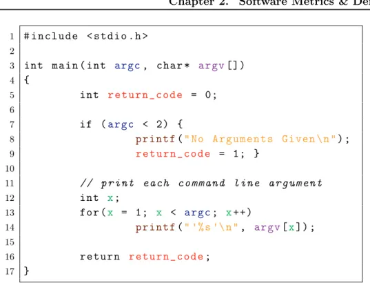
1 # include <stdio .h> 2

3 int main (int argc, char * argv[]) 4 {

5 int return_code = 0;

6

7 if (argc < 2) {

8 printf("No Arguments Given \n");

9 return_code = 1; } 10 11 // p r i n t each c o m m a n d line a r g u m e n t 12 int x; 13 for(x = 1; x < argc; x++) 14 printf(" '%s '\n", argv[x]); 15 16 return return_code; 17 }

Figure 2.1: An example C program.

Perhaps the most well-known static code metrics are based on lines of code (LOC) counts, and give an indication of software size. Consider the C program shown in Figure 2.1. Here there is a single function called main. This function oc-cupies 15 consecutive lines of the containing file; however: 3 of the lines are empty, 2 of the lines contain only a single bracket, and 1 of the lines contains only comments. For these reasons, there are various types of LOC-counts; examples of these include: LOC total, LOC executable, LOC comments and LOC non-blank. Unfortunately, details on precisely what has been measured are often omitted, leading to ambi-guity when LOC-count values are given [Jones 2008]. Problems with traditional LOC-counts also include that they are sensitive to coding style. Looking at Figure 2.1, one or more of the brackets used in the if statement could have been placed on their own line, potentially affecting LOC-count-based measurements. However, such differences may not be of practical importance so long as coding style remains consistent [Rosenberg 1997]. In practice this often leads to code-indentation tools being used prior to metrics collection. Despite the issues with LOC-counts, they are the most frequently used static code metrics, and if measured consistently can provide some insight into software size [Fenton 1998].

While LOC-count-based measures aim to provide insight into software size, an-other set of metrics, proposed by Maurice Halstead in 1977, also aim to provide insight into code complexity and developer effort [Halstead 1977]. The Halstead metrics are based on the following four base measures:

(19)

2.1. Static Code Metrics 7

• The number of unique operators: n1 • The number of unique operands: n2 • The total number of operators: N1 • The total number of operands: N2

Using these base measures the following derived measures can be calculated:

• Halstead Length: N =N1 +N2 • Halstead Vocabulary: n= n1 +n2 • Halstead Volume: V =N ∗ log 2(n)

• Halstead Difficulty: D= (n1 / 2)∗(N2 / n2) • Halstead Level: L= 1 / D

• Halstead Effort: E =D_∗ V • Halstead Content: C = L_∗ V

• Halstead Error Estimate (number of validation bugs): B =V /3000 • Halstead Programming Time (seconds): T =E /18

The length metric is the sum of all operators and operands, and is an alternate size measure to those based around LOC-counts. The vocabulary metric is the sum of all unique operators and operands; code with a high vocabulary is thought to be hard to read and therefore difficult to maintain. The volume metric describes information content in bits, and is another size related measure. The difficulty metric was claimed to measure how difficult the code was to write, and therefore how error-prone it is likely to be. The complement of this is the level metric, with a lower level thought to indicate less error-prone code. The effort metric is used to measure the effort to comprehend and therefore maintain code, while the content metric was claimed to be a language independent complexity measure. Perhaps the most unjustified of these measures are the error estimate and time to program ones, as both include unfounded constants. For the error estimate measure, the proportion of defects within all systems is assumed to be constant, whereas for the time to program measure, the number of programmer elementary mental decisions per second is assumed to be constant. For reasons such as these, the Halstead metrics have been repeatedly and heavily scrutinised [Hamer 1982,Shen 1983,Fenton 1998].

(20)

Metrics concerned solely with code complexity were proposed by Thomas Mc-Cabe in 1976 [McMc-Cabe 1976]. The most well-used of these is known as thecyclomatic complexity,and is based on program control flow. This metric measures linearly in-dependent paths,and is equal to the upper bound of required unit tests forbasis path coverage. Basis path coverage is a white-box testing technique where it is ensured that all executable statements have been run at least once. This is a good starting point when building automated test suites, meaning that cyclomatic complexity has practical worth. Although cyclomatic complexity has direct practical implications, its use as a complexity measure has been widely questioned [Shepperd 1988, Fen-ton 1998]. The main arguments are that it is based on poor theoretical foundations, and that it does not fully capture what is intuitively perceived as complexity.

Other metric suites have been proposed, such as those specifically designed for the object-oriented paradigm [Sommerville 2006,Chidamber 1994]. Such metrics are typically based around degrees of coupling and cohesion, as well as the depth and suitability of inheritance trees. Although defect prediction studies have been carried out using these metrics [Catal 2007], they are not used within this dissertation.

When analysing static code metrics, it is important to know the level of gran-ularity at which they were captured. Common granularities include the file and package level, as well as the module level. In this dissertation the term module is used as a generic term to refer to the function or method level. However, it is worth noting that the term module has different interpretations between authors, which can result in ambiguity during meta-analysis of studies [Hall 2012]. An additional necessity when analysing metrics is to know the programming language of the mea-sured code. This can be more problematic than initially perceived, as many systems comprise more than one language. The varied abstraction levels of programming languages mean that metrics are typically language dependent; for instance, a line of a high-level language (such as Python) will typically achieve more than a line of a low-level language (such as C).

Because static code metrics are calculated through the parsing of source code, their collection can be automated. Thus it is computationally and resourcefully feasible to calculate the metrics of entire software systems, irrespective of their size. Sommerville points out that such collections of metrics can be used in the following contexts [Sommerville 2006]:

• To make general predictions about a system as a whole. For example,

has a system reached a required quality threshold?

• To identify anomalous components. Of all the modules within a

soft-ware system, which ones exhibit characteristics that deviate from the overall average? Modules thus highlighted can then be used as pointers to where developers should be focusing their efforts.

(21)

2.2. Software Defects 9

2.2 Software Defects

Throughout this dissertation the terms: defect, fault and bug are all used inter-changeably. These terms refer to the manifestation of an error in source code, where an error is an erroneous action made by a developer. Faults can be the cause of failures, which occur when users experience undesirable system behaviour at a specific point in time. In general, syntax errors are not regarded as faults; this is because they can be found with far more efficiency by parsers and/or basis path testing. These definitions are based on those given in [iee 1990], although it is worth noting that they are not universally agreed upon [Fenton 1999].

Recording the number of faults found within a unit of software provides a sim-plistic method of partly assessing its quality. However, there are many different types of fault measurement. During software development, the number of bugs found during the testing phase can be recorded. This is an example of pre-release fault measurement; however, post-release (or latent) fault measurement is also pos-sible. The most prevalent form of post-release fault measurement is to record how many failures were experienced up until a specific point in time after a release. It is worth pointing out that such measures are to be used with caution, as the total number of faults within a unit of software (discovered defects +residual defects) is typically never known. This is because of the computational time and complexity required to determine such a value. Therefore, it is folly to assume that a unit of software with many defects removed will be less fault-prone than another with few defects removed, or the converse. Additional problems with such fault counts are that fault severity is not always considered. Although distinguishing fault sever-ity is a challenging task, it is dangerous to have no distinction between trivial and life-threatening faults.

2.2.1 Software Defects & Defect Prediction

In defect prediction experiments, a single fault variable, such as‘the number of faults discovered during system testing’,is typically the dependent variable. In regression experiments, such measurements are often used as is, and the number of faults within each software unit predicted. Note that it is not necessary for the predicted number of faults within each unit to be highly accurate in order for the classifier to be of practical worth. This is because the numbers of predicted faults can be ranked in descending order, producing a ranked list of the seemingly most defect-prone components. Code inspections can then be prioritised around this ordering. It is also possible to normalise the predicted numbers of faults by a size estimator such as LOC total, and then rank the software units in descending order of predicted defect density.

(22)

As well as regression experiments, classification experiments are also increas-ingly popular. Classification experiments involve software units being grouped into categories or classes. Although there is theoretically no limit to the number of classes used in such experiments, two class (or binary) classification experiments are most common. There is typically a ‘defective class’ and a ‘non-defective’ class. Because of this, a pre-processing transformation of the fault count measurements is often required. The most common transformation is to map all software units with no reported faults to the non-defective class, and map all others to the de-fective class. Such a mapping has been carried out in many studies, including: [Menzies 2007b,Lessmann 2008,Elish 2008]. Note that as well as the issue regard-ing fault severity mentioned previously, there is now additionally the issue of fault quantity information being lost. This is clearly a radical simplification, and one that is made solely for the benefit of the learning technique. Although classifica-tion experiments produce categorical predicclassifica-tions, it is often still possible to produce a defect-proneness ranked list of software units, as is the case with regression ex-periments. This is achieved by extracting some internal classifier confidence value associated with each prediction, and then ranking the software units accordingly. There will be more discussion on this in Section5.2.

2.2.2 Defect Measurement

As opposed to static code metrics that can be accurately, quickly and easily ex-tracted, fault measurements are more challenging to obtain. This is because fault measurements are often indirect, rather than direct measurements. A user of a system may be a developer, a tester, or an end user. When such a (human or auto-mated) user experiences a software failure, the occurrence can be recorded. While this typically provides an overall measure of error for the system or subsystem in question, it is often more desirable to obtain fault measurements at a lower level of granularity. This involves the failure inducing fault(s) being isolated and localised, in order to find the offending code unit(s). The level of localisation required de-pends on the level of granularity required. As with static code metrics, common granularities include the package, file, class and module level. Note that it is often possible to aggregate low-level granularity measures to obtain higher level ones.

The most common methods for localising faults involve analysis of the system history recorded in revision control systems. Revision control systems, such as con-current versions system (CVS), record who changed what, when, how, and (ideally) why [Śliwerski 2005]. Such systems enable users to submit a textual message with each commit (set of file changes). The purpose of this message is to describe the changes being made, although there are no guarantees regarding its accuracy. De-spite this, in cases where such messages are consistently entered and of reasonable quality, it is often possible to use them to determine when and where supposed fault-fixes have occurred. This has been carried out in previous studies using sim-ple text-based searches [Mockus 2000,Śliwerski 2005]. After identifying a supposed fault-fix, an assumption can be made that the previous revision to the one in question

(23)

2.2. Software Defects 11

contains faulty code. A more advanced approach than simple text-based searching is known as theSZZ algorithm,and involves progressively working backwards through each previous revision. A search is carried out for the most recent revision(s) to have changed the code being ‘fixed’ in the current revision. If any such revision is found, it is known as a fix-inducing change: a change that caused a ‘problem’ that later needed to be ‘fixed’. The SZZ algorithm was first proposed in [Śliwerski 2005] and later extended in [Kim 2006] & [Williams 2008].

Rather than using revision control log messages alone, the SZZ algorithm was originally proposed to additionally make use of bug reports. Such reports are often maintained throughout the lifetime of a project using purpose built database-backed bug-tracking software. An example of such a software system is Bugzilla1. For projects that have utilised such a system, the process for localising faults described above can be extended. Searching for all bug reports that have been assigned the ‘fixed’ status results in a set of unique bug identifiers. As it is common practice for developers to include a bug report number in the commit message of a ‘bug fix’ [Śliwerski 2005], commit messages can be searched for these identifiers, in addition to other indicators of a fault-fix (such as the word: ‘fixed’). This is claimed to increase the precision achieved when using log messages alone [Śliwerski 2005], resulting in more confidence as to whether or not a commit was an intended fault-fix.

An alternative method for identifying fault-fixing revisions was proposed in [Os-trand 2005], following a recommendation by developers. This simple approach clas-sifies revisions using information regarding the number of files changed in each com-mit. Commits containing one or two changed files are classified as fault-fixing, all others are considered not so. Although this method is very simplistic, it was claimed to work well with a sample of the proposing authors’ data [Ostrand 2005]. The main advantage of this method is that it can be used in cases where commit messages have not been entered appropriately.

Perhaps the most accurate way to determine whether or not a commit is an intended fault-fix is to manually classify the textual difference between it and its previous revisions. This method requires an expert and is labour intensive, often making it infeasible even for small systems. The automated methods previously described were motivated by this frequently encountered infeasibility. Although manual classification is likely the most accurate way to classify commits, “it is very difficult to reliably extract fault-fixing data from change repositories” [Hall 2010]. This is because of the expertise required to do so, the subjective nature of manually classifying fault-fixes, and also because the historical data may be lacking in quality. The issues involved in extracting fault data from change repositories are revisited in Chapter 7, which contains a description of the work undertaken to extract fault data from the Barcode open-source system.

1

(24)

(25)

Chapter 3 Machine Learning

Contents

3.1 Supervised Learning. . . 14 3.2 Basic Learning Techniques . . . 15 3.2.1 Instance-Based Learning. . . 15 3.2.2 Linear Separators. . . 19 3.2.3 Tree-Based Learning . . . 20 3.2.4 Bayesian Classifiers. . . 22 3.3 Assessing Predictive Performance . . . 24 3.3.1 Training & Testing Sets . . . 24 3.3.2 Categorising & Quantifying Predictions . . . 25 3.3.3 Measuring Class-Specific Error . . . 27 3.4 The Class Imbalance Problem . . . 32 3.5 Model Optimisation . . . 34 3.6 Support Vector Machines . . . 37

(26)

14 Chapter 3. Machine Learning

M

achine learning, which is closely related to data mining, is a broad area of computer science regarding algorithms that enable computers to learn [Segaran 2007]. This often involves “the extraction of implicit, previously unknown, and potentially useful information from data” [Witten 2005]. Perhaps the most popular area of machine learning issupervised learning,where predictions are made regarding future events based on knowledge of past events. Another popular area of machine learning is unsupervised learning, which is concerned with finding hidden structure within data. Machine learning is possible because almost all non-random data contains underlying patterns [Segaran 2007]. When these patterns are discov-ered they can then be exploited.

This chapter begins with an introduction to supervised learning, or learning by example. Basic supervised learning techniques are then described, those most rele-vant to this dissertation. Methods to assess the predictive performance of classifiers are discussed in Section 3.3, where the main difficulties are introduced. Section3.4 leads on from this with a brief introduction to the class imbalance problem. The process of classification model optimisation is detailed in Section 3.5, a process key to successful utilisation of many classification methods. A family of such classifica-tion methods are described in Secclassifica-tion 3.6, namely, support vector machines. These highly sophisticated classifiers have been heavily used and are extensively referred to throughout this dissertation.

3.1 Supervised Learning

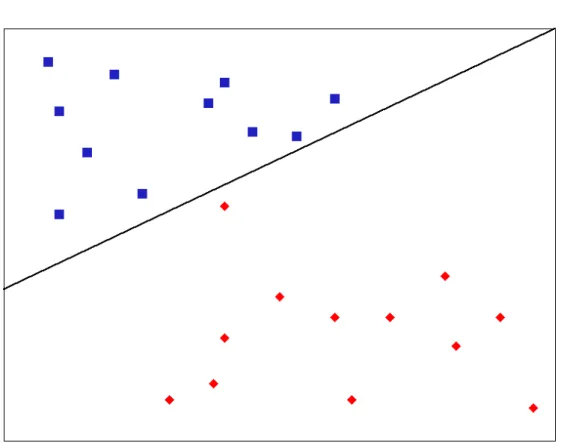
Supervised learning is a discipline of machine learning, which is in turn a sub-discipline of artificial intelligence. Supervised learning algorithms are trained using labelled data. Such data (x) comprises p features (or attributes) and q feature vectors (vectors hereafter). Additionally, there are q class labels (labels hereafter), each one corresponding to a single vector. The concatenation of a vector with its label is known as an instance or data point. Although it is possible for a label to comprise multiple values, this is not considered in this dissertation. If the labels within a data set form a set of nominal values, then this is considered aclassification problem, whereas if the labels form a set of continuous values, this is considered a regression problem. In this dissertation the main focus is on classification problems where the cardinality of the set of labels is two. This is known accordingly as binary classification. Example training data suitable for a binary classifier is shown in Table 3.1. This data comprises: two features (lines of code and cyclomatic complexity), six feature vectors, and their six corresponding labels. Each data point describes two quantitative features of a software unit (the independent variables), as well as whether or not that software unit caused any operational failures (the dependent variable). This data is suitable for a two class (binary) classifier, as the set of labels consists of two elements.

(27)

3.2. Basic Learning Techniques 15

Lines of Code Cyclomatic Complexity Defects?

7 1 No 500 31 Yes 5 2 No 12 3 Yes 84 6 No 90 13 No

Table 3.1: Example data suitable for a supervised learning algorithm.

The aim of supervised classification learning methods is to use labelled data to generate a mapping functionf(x) such that when a vector is presented, its correct label is returned. Minimising the error of this process is often the most important learning algorithm criteria. The data used in this process should be a representative sample from the specific problem domain. However, only a very small proportion of all possible instance combinations (theinput space) is typically contained within the available data. Therefore, learning methods are required to generalise in order to successfully predict unseen data, data that was not used while constructing the classifier, but that will almost certainly be found in the real world. Generalisation is therefore very often the key to successful data mining.

3.2 Basic Learning Techniques

3.2.1 Instance-Based Learning

Instance-based (or case-based) learning requires each and every training instance to be stored verbatim [Witten 2005]. Such algorithms are said to be lazy, as rather than building a classification model during initial training from which all predictions are based, the original training data must instead be consulted for each prediction. The main advantage of this is that training data can be added, removed or modified dynamically. Disadvantages are that large data sets can result in slow algorithm operation, and that there is no classification model from which new knowledge can be easily extracted (as can be the case with decision trees (Section3.2.3), for example). For all but the most simple forms of instance-based learning, generalisations can occur. This is via a search for the most similar vector(s) to the one being classified. Similarity is typically determined by a distance function, with the corresponding label(s) of the nearest vector(s) to the one being classified used to determine the prediction made. The assumption is that instances of the same class will be rela-tively nearby in the feature space. The distance function used depends on the type of features contained within the data. For numeric features (such as those used throughout this dissertation), the most common distance function is the Euclidean distance. This is defined in Equation 3.1, where the distance between two vectors (xi and xj) is calculated using allp features.

(28)

16 Chapter 3. Machine Learning Euclidean_Distance(xi,xj) = v u u t p X d=1 xd_i −xd_j 2 . (3.1) 3.2.1.1 Rote Learning

Rote learning, or learning by memorisation, is one of the simplest forms of supervised learning [Noyes 1992]. Rote learning involves the storage of training data into some form of database. When required this data can then be recalled, potentially with great efficiency. The limitation of rote learning is that only vectors included in the training data can be classified. This is because the training data has only been stored, no attempt to infer or generalise has been made. For this reason rote learning systems are mainly used where the correct label for every possible combination of features is known beforehand. This situation is not stereotypical of machine learning problem domains. However, rote learning systems can additionally be used as components of ensemble learning methods, perhaps to efficiently classify parts of the input space where the correct labels are known.

3.2.1.2 Nearest-Neighbour-Based Learning

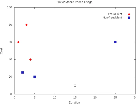
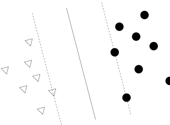
An extended and far more robust classification method than rote learning is nearest-neighbour-based learning. The most basic nearest-nearest-neighbour-based learning algo-rithm isone-nearest-neighbour. This algorithm performs the same outward function as rote learning for cases where the test vector is included in the training data. When this is not the case, the training data is searched for the instance whose dis-tance to the test vector is minimal. The test vector is predicted as belonging to the same class as the instance found, its nearest-neighbour (see Figure 3.1).

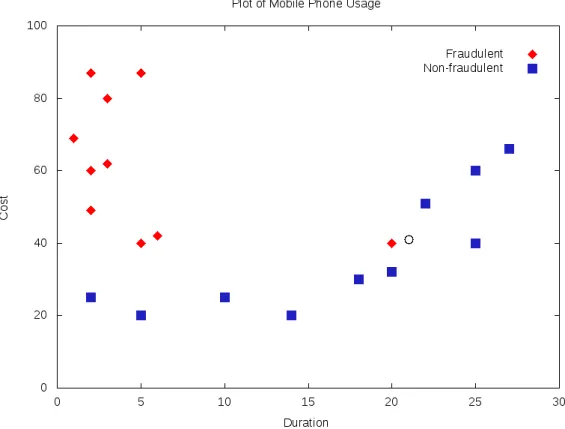
The more general form of this concept isk-nearest-neighbour,wherek≥1nearest training instances are found, and a majority vote is taken on the class of the test vector. Accordingly,k should be defined as an odd number for binary classification problems, to prevent ties during voting. The potential benefit of using a higher value of k is that it results in a clearer picture of whereabouts in the data space the test vector lies. This is because more information regarding the test vector’s surrounding instances is taken into account (see Figure 3.2). The optimal value of k is data specific, and typically cannot be known a priori. However, a model optimisation phase (see Section3.5) may be used to aid its estimation.

Although intuitive and easily comprehensible, nearest-neighbour-based learning methods are very sensitive to both noise (incorrect or erroneous data) and irrel-evant attributes (those that are uncorrelated with the class). This is because all features typically have an equal weight when similarity is determined (see Equation 3.1). Because of this, data cleansing is often a prerequisite to successfully using such techniques, and cleansing methods specific to instance-based learners have been proposed [Segata 2010, Segata 2009]. An additional problem with nearest-neighbour-based learners is that they are very sensitive to the class distribution of

(29)

Figure 3.1: An example of the (one) nearest-neighbour algorithm. Here is a plot of genuine and fraudulent mobile phone usage. The two features are call cost and call duration. Fraudulent calls are represented by diamonds whereas non-fraudulent calls are represented by squares. The test data (represented by a circle) is predicted as belonging to the non-fraudulent class, as this is the class of its nearest data point.

(30)

Figure 3.2: Another k-nearest-neighbour example. Although the test vector (rep-resented by a circle) appears to be more similar to the non-fraudulent class, k will need to be 3 or more for this to be the prediction. Note that the fraudulent example nearest to the test vector is anoutlier,as it is not representative of its class. It may be that this data point has an incorrect label, perhaps due to a data quality issue.

(31)

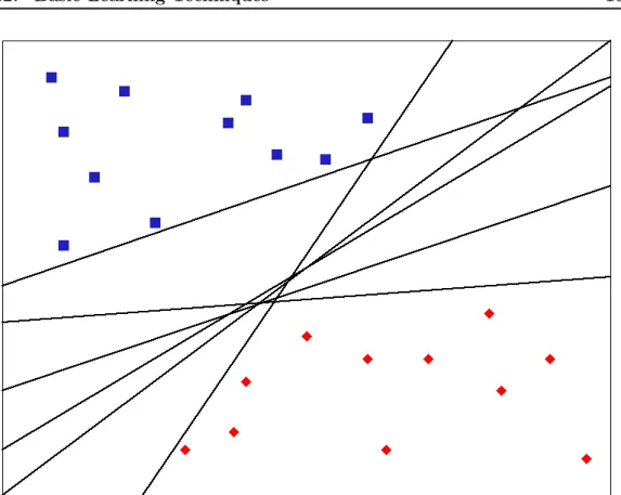
Figure 3.3: Some of the possible separating lines of a linear separator.

the training data. If the majority class (the class that appears most often in the training data) contains 90% of instances, the probability of having a majority class neighbour is higher than the probability of having a minority class nearest-neighbour. In such cases, the majority class will usually be over-predicted, meaning that potentially all test vectors will be predicted as belonging to the majority class.

3.2.2 Linear Separators

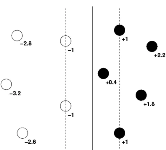
Linear separation techniques usually involve using linear combinations of numeric features to separate classes. An example of this is shown in Figure 3.3. In this figure, several possible linear separators are shown, all of which separate both classes without error. An example of an algorithm that can generate such separators isthe perceptron [Rosenblatt 1958]. It follows that this is a non-deterministic algorithm, as there are many possible solutions shown in Figure 3.3. In fact, there are an infinite number of solutions to this problem.

Although each of the separators shown in Figure3.3separate both classes with-out error, we ideally wish to maximise performance on unseen data, not simply the training data. The most intuitive way to try and ensure best performance on un-seen data is to have a separator with a largemargin, a large distance between both classes. Having a large-margin separator, as opposed to a small-margin separator, generally results in improved performance on unseen data.

(32)

Because margin size is so influential to generalisation ability, it may be beneficial for predicting unseen data to have a non-perfect separator. This is a separator where there are training instances which fall on the wrong side, the side that is not shared with the majority of their class. Methods which do not allow this to occur produce hard-margin separators, whereas methods which do allow this to occur produce soft-margin separators. The difference between these two types of separators is shown in Figure 3.4.

Hard-margin separators generally do not involve parameters; however, soft-margin separators typically require a slack parameter to determine the trade-off between minimising the training error and maximising the size of the margin. This is known as thecost orc parameter, and is tunable to user requirements. A low cost value generally results in many training errors and a large margin, whereas a high cost value generally results in few training errors and a small margin. In fact, cases where c = ∞ are conceptually identical to hard-margin separators. The optimal value of cis data dependent, and is often estimated using a systematic search (see Section3.5).

The main disadvantage of linear separators is that they are limited to linearly separable problems. However, many problems are linearly separable, especially when there are a large number of features (resulting in a high-dimensional space). The main advantages of linear separators are that they are easily comprehensible and computationally efficient, in that they are suitable for huge data sets with large numbers of features.

3.2.3 Tree-Based Learning

Tree-based (or decision tree) learning algorithms produce a structured classification model during initial training on which all predictions are based. Such methods are said to be eager, as all computation regarding future predictions is made in the training period (the raw training data is not revisited at classification time). A recursive, top-down method is usually employed to construct trees. This is known as the divide-and-conquer approach [Witten 2005], and can be solved recursively. The top (or root) node branches (or splits) at the feature which best separates the data into homogeneous subsets with the same label. Various methods exist for determining this feature; however, the most well-known decision tree algorithms use either entropy [Quinlan 1993] or Gini index [Ceriani 2011] based measures. An example graphical representation of a decision tree is shown in Figure 3.5. This figure shows a possible decision tree that sailors could use to determine whether or not it is safe to sail under certain conditions. In this figure it can be seen thatWind Speed (mph) is the feature at the root node, and that its test condition is whether or not it is greater than 22. If it is, a prediction of Don’t Sail is made. If it is not, the test condition at the following node is evaluated. This process continues until a prediction is made. Therefore, each prediction can be seen as the conjunction of one or more simple test conditions.

(33)

(a) Hard margin. All training data is correctly classified, but with a small margin.

(b) Soft margin. By allowing training error, the size of the margin is increased.

(34)

Wind Speed (mph)

> 22 Don't Sail <= 22

Temperature (°C)

Don't Sail <= 6 Sail > 6

Figure 3.5: An example decision tree.

3.2.3.1 Random Forests

Random forest classifiers are strictly an ensemble classification method, but they are introduced in this section as they are comprised solely of multiple decision trees. A random forest classifier comprises two or more CARTs (classification and re-gression trees) and utilises a bootstrap aggregating (orbagging) ensemble approach [Breiman 2001]. Additionally, each of the trees are said to berandomised, as they only train on a random subset of a < p features (where p is the total number of features available). The mode classification across all individual classifiers is taken as the final prediction for each test vector.

Bagging is an ensemble approach whereby each individual node (or tree in this case) is equally weighted in the final prediction [Breiman 1996]. Other ensemble approaches, such as boosting, differ from this as they weight each node judging by past performance. To encourage variation in the results of nodes, the bagging approach provides each node with a sampled version of the training data. This bootstrap sample is both uniform and of the same size as the original sample. It is also made by replacement,resulting in many training instances being repeated, and some not making it into the new sample. Separate to bagging, but also designed to encourage variation in results, is the method of passing a random subset of training features to each node. This technique is known as randomisation. Combining the power of multiple decision trees by using random forests “often produces excellent predictors” [Witten 2005].

3.2.4 Bayesian Classifiers

A Bayesian (or Bayes) classifier is a linear classification technique based on Thomas Bayes’ theorem. This theorem (presented in Equation 3.2) is concerned with prob-ability theory, and provides a method to determine conditional probabilities.

(35)

Pr(hypothesis_|evidence) = Pr(evidence|hypothesis)×Pr(hypothesis)

Pr(evidence) (3.2)

Perhaps the most popular Bayes classifier is the naïve Bayes algorithm, so-called because of the simple but often false assumption ofconditional independence,where every feature is assumed to be fully independent. Despite this assumption, naïve Bayes classifiers have been reported to perform competitively with far more sophis-ticated techniques [Huang 2003]. Similar to instance-based learners, naïve Bayes classifiers can be updated over time, allowing model evolution. Unlike instance-based learners however, naïve Bayes models are independent of the training data (it does not require storage). Because of this, and low computational demands, naïve Bayes is a suitable method for potentially huge, constantly evolving domains, where timely execution may be required. An example of such a domain is that of spam email classification, where naïve Bayes classifiers have been extensively used [Vangelis Metsis 2006].

During training, naïve Bayes classifiers use basic statistical properties of each feature to determine their probabilities of association with each class. The advantage of this is that models can be easily interpreted, as the probabilities for each feature are stored explicitly. This ease of human interpretation of the inner workings of the model makes naïve Bayes a white-box classification method. This is similar to both tree-based and instance-based learners, amongst others. White-box methods are typically preferable to black-box methods, as it is always possible to discover the reasoning for each prediction made. Additionally, new knowledge can potentially be discovered via model analysis. In the case of naïve Bayes, this would involve examining the probabilities associated with each feature.

Naïve Bayes classifiers determine, for each test vector, a probability of associ-ation with each class. Note that these are not strictly probabilities, but can be conceptualised as them nonetheless. In the simplest of implementations, the class with the highest probability will be the predicted class. However, many implementa-tions include a user-tunabledecision threshold parameter. For binary classification tasks, this is described as follows. If the probability of association with the class of most interest is greater than the decision threshold, then this will be the predicted class. Otherwise, a prediction of the opposing class is made. Therefore, the decision threshold effectively controls how eager (or not) the classifier is to make predictions of a certain class.

(36)

3.3 Assessing Predictive Performance

Assessing the predictive performance of a classifier is more complicated than may be initially perceived. For rote learning methods where no generalisation takes place, the quality of predictions is clearly a direct result of the quality of the training data. For this reason, algorithm speed is often the performance criteria assessed, rather than predictive ability. As this is not a focus of this dissertation, it is not discussed further. This section instead describes ways in which the predictive performance of a classifier can be quantified.

3.3.1 Training & Testing Sets

When assessing the performance of a classifier, the most common aim is to acquire an estimate of how well it could potentially perform in the real world. Because (as mentioned at the start of this chapter) only a very small proportion of the input space is typically contained within the available data, it is often entirely unrealistic to assume that a classifier deployed in the real world would be required to classify vectors included in the training data. For this reason, classifiers are required to be tested onunseen data: data that was not usedin any way during classifier construc-tion. Failure to adhere to this principle often results in an optimistic approximation of potential real-world performance [Witten 2005]. This is because the classifier has already learnt from the ‘correct’ label of each seen test vectors, and therefore has an unfair and often unrealistic advantage.

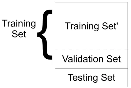
A classifier deployed in the real world would usually be constructed using all available data for the specific problem domain. Each prediction made by the system would then have to be (often manually) validated, which is typically a resource intensive task. To avoid this resource intensive process while classifier feasibility is being explored, an estimate of potential real-world performance is obtained instead, using only the data already available. A simple method of doing this is known as a holdout, where x% of available data is used for constructing a classifier, while the remaining(100₋x)%is kept separate during classifier construction, and used to test how well the classifier can generalise. Thus, these subsets of data become known as a training set and a testing set, respectively (note that these are not mathematical sets). For both these sets to be fully independent of each other, and contextually valid, they must share no common instances. The classifier is trained on the training set, and performance on the independent test set is used as the estimate of potential real-world performance. Some of the various methods of measuring performance will be explained in the next few sections. In order to defend against statistical bias, the holdout process is often repeated many times, with different training and testing set samples pseudo-randomly chosen. The average performance for each holdout experiment is then reported as the final, overall performance.

A more sophisticated method than a simple holdout is known as a stratified holdout, where the training and testing sets both maintain an approximately equal class distribution to the one in the original sample. Imagine there are 1000 labelled

(37)

3.3. Assessing Predictive Performance 25

data examples available in the domain of jet engine failure prediction. There are only 100 examples where the engines failed, all others are examples of non-failures. With a two-thirds training, one-third testing holdout, it is possible (as an extreme example) that the 667 training instances contain none of the engine failure exam-ples. Supervised learners, by definition, require labelled examples in order to learn. Therefore, a classifier trained on such data would have little chance at predicting any engine failures, and would instead be expected to predict every test vector as belonging to the majority class (non-failures). A stratified holdout would be much more effective in such an imbalanced domain. With a stratified holdout, two thirds of each class would be contained in the training data, and one third of each class in the testing data. As long as the original data sample is representative of the prob-lem domain, this is a much more effective way of obtaining estimates of potential real-world performance.

Although repeating the stratified holdout process many times alleviates the bias issue, potential problems remain. Repeating the process too few times may result in some instances never being included in a testing set. Additionally, testing sets will overlap, meaning that classifiers will be presented with some test vectors more times than others. Both of these issues can introduce bias. To address these issues, k-fold cross-validation can be used. In k-fold cross-validation,k >1 approximately equal sized and mutually exclusive sub-samples (or folds) are created from the original sample [Kohavi 1995]. Then, k holdout-style experiments are carried out, where one of the folds is the testing set, and all others combined are the training set. Each fold has one turn as the testing set, and final performance is reported as the average across allkfolds (see [Forman 2010] for important details on how this average should be calculated). Stratified k-fold cross-validation is an extension to this method, where each fold maintains a similar class distribution to the original sample, as previously described. To further reduce bias, the stratified cross-validation process can be repeated many times, with different sub-samples pseudo-randomly chosen. Final performance is then calculated as the average of all individual cross-validation averages. Although cross-validation is computationally expensive, it is fairly stable and unbiased for adequately sized data sets, where k is reasonably large (10 folds has been recommended [Kohavi 1995]).

3.3.2 Categorising & Quantifying Predictions

Because the testing sets in such classification experiments are artificial (they are not real unknown vectors, but simulations of them), the label for each test vector is already known. Clearly, to make the task of a classifier worthwhile, these test labels are not used during the classification process. After this process is complete however, they are used to assess how well the classifier has performed, or in other words, how the predictions made by the classifier correspond with the ‘correct’ labels.

Perhaps the most intuitive way to quantify predictive performance is to deter-mine the proportion of correct classifications. The pseudo-code for this is shown in Figure3.6. This figure shows an attractive as well as intuitive solution, as it scales

(38)

no_correct = 0 # initialise the no. of correct classifications for test_vector in test_set:

if test_vector.real_label == test_vector.predicted_label: no_correct += 1

print no_correct / test_set.size

Figure 3.6: Pseudo-code for calculating the correct classification rate.

robustly regardless of the number of classes in the data. The metric describing the proportion of correct classifications is known as accuracy, or correct classification rate (CCR). Its complement is known aserror rate,and is defined as (1−accuracy). These correct/incorrect classification rate measures are suitable when the class dis-tribution of the test data is equal (or balanced), and when themisclassification cost for each class is also equal. An example of such a domain is optical transmission error detection, where a classifier attempts to detect bit-errors in the transmission of a digital signal. In this domain it is assumed that there will be an equal number of zeros and ones transmitted over a communication medium over time. It is also assumed to be illogical to favour the correct transmission of a zero over the correct transmission of a one. For these reasons, overall correct/incorrect classification rate measures are suitable in such a domain, and a value of approximately 0.5 is the threshold for a classifier of any practical worth. This is because when there are an equal number of test vectors originally labelled as belonging to each class, predicting all test samples solely as being in either one class or the other will result in such a performance figure. Additionally, any such performance figure (not equal to 0 or 1) provides no information toward whether there were more errors in one class than another, which is not a necessity in such a domain.

Accuracy and error rate are both measures which favour the majority class. Because of this, they are not suitable in domains where there is an imbalanced class distribution. To demonstrate, we will revisit the jet engine failure prediction scenario described earlier in this section, where there were 1000 examples of which only 100 were in the minority class. If this data set were a test set, a classifier predicting every test vector as belonging to the majority class would achieve a near-optimal accuracy (0.9), even though the classifier is of no practical worth. This scenario is also appropriate for demonstrating the other limitation of such measures. Mistakenly predicting a jet engine that is not about to fail as being about to fail will result in unnecessary servicing of the engine, which is a waste of resources. However, mistakenly predicting a jet engine which is about to fail as not being about to fail could result in an operational failure, with far more serious consequences. Accuracy-like measures give no information toward class-specific error, only overall error. For these two reasons, they would be entirely unsuitable in such a domain.

(39)

3.3.3 Measuring Class-Specific Error

To overcome the problems of accuracy-like measures, class-specific error must be measured. In a binary classification task, the two classes are commonly referred to as the positive class and the negative class. There is a symmetry between these classes; however, the positive class typically refers to the class of most interest, which is often the minority class. For each test vector predicted during a binary classification experiment, there is exactly one of four possible outcomes:

• Atrue positive (TP)occurs when a data point labelled as positive is correctly predicted as positive.

• Atrue negative (TN)occurs when a data point labelled as negative is correctly predicted as negative.

• Afalse positive (FP) occurs when a data point labelled as negative is incor-rectly predicted as positive.

• Afalse negative (FN) occurs when a data point labelled as positive is incor-rectly predicted as negative.

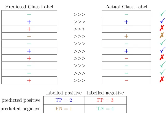
Collections of these values can be put into aconfusion matrix,as shown in Figure 3.7. Such a confusion matrix forms the basis of how the predictive performance of binary classifiers are often quantified (see Figure 3.8). Most classifier performance measures are based on simple equations of the four comprising raw measures (TP, TN, FP and FN). In addition to determining predictive performance, these values can also provide contextual insight into the test data. Imagine a confusion matrix generated during a single holdout experiment. Using the values in the confusion matrix alone, the number of test vectors originally labelled as belonging to the positive class can be determined as P OS=T P +F N. It follows that the number of test vectors originally labelled as belonging to the negative class is determined as N EG = T N +F P. Therefore, the total number of vectors in the test set is determined as|T est|=N EG+P OS=T P +T N+F P +F N.

labelled positive labelled negative

predicted positive TP FP

predicted negative FN TN

Figure 3.7: A confusion matrix.

To provide a more concrete example of a confusion matrix, we will again use the jet engine failure prediction example. There are 100 positive (minority) class data points in this data set and 900 negative (majority) class data points. If this data set were a test set and we predicted everything as being in the majority class, we would obtain the confusion matrix shown in Figure3.9. As already stated, accuracy is not a suitable measure for this example; however, using the confusion matrix alone, we can computeaccuracy as(T P+T N)/(T P+T N+F P+F N). Although

(40)

Predicted Class Label Actual Class Label

− >>> −

X

+ >>> +

X

+ >>> −

7

− >>> +

7

− >>> −

X

+ >>> +

X

+ >>> −

7

− >>> −

X

− >>> −

X

+ >>> −

7

labelled positive labelled negative predicted positive TP = 2 FP = 3

predicted negative FN = 1 TN = 4

Figure 3.8: The confusion matrix for a toy example.

the near-optimal accuracy of 0.9 may intuitively appear as though our classifier has performed very well, in this domain we need to examine class-specific performance to determine potential real-world performance. One such suitable measure to aid with this is known as sensitivity (orrecall ortrue positive rate). This measure describes the proportion of test vectors originally labelled as belonging to the positive class that were correctly classified. To calculate sensitivity we useT P/(T P+F N). In this example this yields a sensitivity of 0, showing that no minority class test vectors were correctly predicted. We can work out a similar measure for the negative class, known as specificity (ortrue negative rate). We determine this usingT N/(T N+F P). In this example the specificity is 1, showing that all majority class test vectors were correctly predicted. Perfect classification is achieved when there is a sensitivity and specificity of 1, which implies that there is also an accuracy of 1. A trade-off typically exists between sensitivity and specificity, and is explained as follows. To achieve an optimal sensitivity, all test vectors appearing to belong to the positive class must be predicted as such. However, for every prediction made, there is a risk of misclassification. Making an incorrect positive prediction means a data point originally labelled as negative has been incorrectly predicted as positive. Such a false positive will lower the specificity, which we are aiming to maximise along with sensitivity. Thus, trying to optimise one of these measures often compromises the other. It is worth pointing out that these measures, which originate from the medical sciences, are designed to be used together and complement each other. As shown in this example, obtaining an optimal specificity is simply a case of making only negative predictions. Similarly, an optimal sensitivity can be achieved by making only positive predictions. Both such predictors clearly have little practical worth.

(41)

labelled positive labelled negative predicted positive TP = 0 FP = 0 predicted negative FN = 100 TN = 900

Figure 3.9: A confusion matrix with only negative-class predictions.

The trade-off between sensitivity and specificity can be visualised using areceiver operating characteristic (ROC) graph. ROC graphs were first used during World War II to analyse radar signals; there use in machine learning began much later in 1989 [Spackman 1989]. A ROC graph is a two-dimensional plot, with sensitivity on the y-axis and(1₋specif icity) on the x-axis. The use of (1₋specif icity), also known as the false positive rate or type 1 error rate, means that an optimal classifier will be shown on a ROC graph as having a sensitivity (or true positive rate) of 1, and a false positive rate of 0. Imagine a naïve Bayes classifier tested on the same test set three times. Each time the classifier will use a different decision threshold (see Section 3.2.4) taken from the set {0.4, 0.5, 0.6}. After this process, there will be three sets of results, all in the form of confusion matrices. From these confusion matrices, we can plot three points on a ROC graph, as shown in Figure 3.10. If we continued this process for every possible decision threshold, we would end up with a ROC curve,as shown in Figure 3.11. This figure demonstrates the trade-off between sensitivity and specificity for this particular classifier on this particular test set, as the decision threshold is varied. An interesting point in ROC space is point {0,0}, where the classifier makes no positive predictions, and therefore has no true or false positives. The complement of this is at point {1,1}, where the classifier makes only positive predictions, and therefore has no true or false negatives. As already stated, optimal performance is at point {0,1}. In practice, classifiers rarely achieve such performance; however, curves often bend upwards towards this ideal point. Also worthy of discussion in Figure 3.11 is the straight, x = y dashed line. Any point situated below this line demonstrates performance that is worse than random [Flach 2003]. In fact, inverting the predictions made by such a classifier yields better performance, and moves the point to its corresponding position (reflection) above the dashed line.

ROC curves can be useful for classifier comparisons; if two classifiers often have similar performance in a specific domain, inspection of their ROC curves can il-luminate which one performs best in specific regions of ROC space. Additionally, ROC curves can show which method is more sensitive to decision threshold setting. To compare multiple classifiers in terms of their ROC curve performance without the need for visual inspection, the area under the ROC curve (AUC-ROC, or more commonly simply AUC) can be computed. This is a value between 0 and 1, with 1 indicating optimal performance.

(42)

30 Chapter 3. Machine Learning 0 0.2 0.4 0.6 0.8 1 0 0.2 0.4 0.6 0.8 1

True Positive Rate

False Positive Rate

0.4 0.5 0.6

Figure 3.10: A ROC graph containing three points. The true positive rate, also known as sensitivity or recall, is on the y-axis. The false positive rate, also known as type 1 error rate or (1₋specif icity), is on the x-axis.

(43)

3.3. Assessing Predictive Performance 31 0 0.2 0.4 0.6 0.8 1 0 0.2 0.4 0.6 0.8 1

True Positive Rate

False Positive Rate

0.4 0.5 0.6

Figure 3.11: A ROC curve. The three points from Figure 3.10 are shown for ref-erence. Each pixel comprising the solid line corresponds to the classifier’s perfor-mance with a unique decision threshold. The perforperfor-mance for every possible decision threshold is shown on this line.