COUPLED COASTAL FORECASTING SYSTEMS
A Dissertation by
GAURAV SINGHAL
Submitted to the Office of Graduate Studies of Texas A&M University
in partial fulfillment of the requirements for the degree of DOCTOR OF PHILOSOPHY
August 2011
COUPLED COASTAL FORECASTING SYSTEMS
A Dissertation by
GAURAV SINGHAL
Submitted to the Office of Graduate Studies of Texas A&M University
in partial fulfillment of the requirements for the degree of DOCTOR OF PHILOSOPHY
Approved by:
Co-Chairs of Committee, Vijay G. Panchang James M. Kaihatu Committee Members, Billy L. Edge
Gerald E. Hite Head of Department, John Niedzwecki
August 2011
ABSTRACT
Viability, Development, and Reliability Assessment of Coupled Coastal Forecasting Systems. (August 2011)
Gaurav Singhal, B.Tech., Indian Institute of Technology, Kharagpur, India; M.S., Texas A&M University
Co–Chairs of Advisory Committee: Dr. Vijay G. Panchang Dr. James M. Kaihatu
Real-time wave forecasts are critical to a variety of coastal and offshore opera-tions. NOAA’s global wave forecasts, at present, do not extend into many coastal regions of interest. Even after more than two decades of the historical Exxon Valdez disaster, Cook Inlet (CI) and Prince William Sound (PWS) are regions that suffer from a lack of accurate wave forecast information. This dissertation develops high-resolution integrated wave forecasting schemes for these regions in order to meet the critical requirements associated with shipping, commercial and sport fishing vessel safety, and oil spill response. This dissertation also performs a detailed qualitative and quantitative assessment of the impact of various forcing functions on wave pre-dictions, and develops maps showing extreme variations in significant wave heights (SWHs). For instance, it is found that the SWH could vary by as much as 1 m in the northern CI region in the presence of currents (hence justifying the need for integration of the wave model with a circulation model). Such maps can be use-ful for several engineering operations, and could also serve as a guidance tool as to what can be expected in certain regions. Aside from the system development, the issue of forecast reliability is also addressed for the PWS region in the context of the associated uncertainty which confronts the manager of engineering operations or other planners. For this purpose, high-resolution 36-h daily forecasts of SWHs are compared with measurements from buoys and satellites for about a year. The
results show that 70% of the peak SWHs in the range 5-8 m were predicted with an accuracy of 15% or less for a forecast lead time of 9 h. On average, results indicate 70% or greater likelihood of the prediction falling within a tolerance of ±(1*RMSE) for all lead times. This analysis could not be performed for CI due to lack of data sources.
ACKNOWLEDGMENTS
First and foremost, I would like to extend my gratitude to Dr. Vijay Panchang for graciously accepting me as his PhD student in Fall 2007. Dr. Panchang provided continuous support and motivation throughout my research work. I am also grateful to Dr. James Kaihatu for willingly serving as the co-chair of my committee, and for providing insightful comments throughout my research.
I would also like to thank my committee members Drs. Billy Edge and Gerald Hite for their helpful suggestions/comments towards my doctoral research. Thanks also go to Drs. Martin Miller, Juan Horrillo, Carl Schoch, Ayal Anis, Zeki Demir-bilek, and Earl Hayter. I would also like to thank NOAA, TIO, and Texas A&M Galveston’s Research and Graduate Office for partial funding support.
I have also been blessed to have the support of a number of colleagues and friends throughout my research. I would like to thank Chan Kwon, Abhishek, Ashwin, Myoung Keun, Bo, Emily, Keith, Jitendra, Waqar, Puneet, Praveen, Sarabjyot, Veera, Prasenjit, Anuja, Rohit, and all others that I may have missed. I am also extremely grateful to the Gifford and Lewis families for graciously including me in several of their family holiday dinners.
Last but not the least, I am extremely grateful to my parents, elder brother Manish, sister-in-law Nisha, and nephew Kaushal for providing unconditional love and support throughout the course of my education. Without their sacrifices, I would not have made it thus far.
TABLE OF CONTENTS
Page
ABSTRACT . . . iii
DEDICATION . . . v
ACKNOWLEDGMENTS . . . vi
TABLE OF CONTENTS . . . vii
LIST OF TABLES . . . x
LIST OF FIGURES . . . xi
1 INTRODUCTION AND LITERATURE REVIEW . . . 1
1.1 Historical background. . . 3
1.2 Overview of operational forecasting . . . 6
1.3 Literature review . . . 8
1.3.1 Hindcast vs. forecast . . . 10
1.4 Research objectives . . . 11
2 OVERVIEW OF WAVE AND CIRCULATION MODELS . . . 15
2.1 Wave model . . . 15
2.2 Circulation model . . . 16
2.3 Background on wave-current interaction . . . 18
2.3.1 Effect of currents on waves . . . 19
2.3.2 Effect of waves on currents . . . 19
3 DEVELOPMENT OF INTEGRATED WAVE FORECASTING SCHEME FOR COOK INLET, ALASKA . . . 23
3.1 Introduction . . . 23
3.2 Bathymetric information and available datasets . . . 27
3.3 Surface weather patterns . . . 28
3.4 Surface-current patterns and modeling . . . 32
3.5 Surface wave-patterns and modeling . . . 44
3.6 Coupled wave-current modeling . . . 46
3.7 Results: Application of coupled wind-wave-current modeling . . . 49
Page
3.7.2 Quantitative analysis of coupled schemes . . . 64
3.8 Discussion . . . 65
4 SENSITIVITY OF FORCING FUNCTIONS ON WAVE PREDICTIONS IN COOK INLET, ALASKA. . . 70
4.1 Introduction . . . 70
4.2 Sensitivity to modeled currents . . . 71
4.3 Sensitivity to open boundary conditions . . . 74
4.4 Sensitivity to winds . . . 80
4.5 Discussion . . . 83
5 HIGH-RESOLUTION COUPLED MODELING IN KACHEMAK BAY RE-GION . . . 87
5.1 Introduction . . . 87
5.2 Bathymetric data and features . . . 89
5.3 Coupled wave-circulation model for KB . . . 90
5.4 Discussion . . . 99
6 DEVELOPMENT OF WAVE FORECASTING SCHEME FOR PRINCE WILLIAM SOUND, ALASKA . . . 101
6.1 Introduction . . . 101
6.2 Available data . . . 105
6.3 Development of PWS forecasting system . . . 106
6.4 Transition to operational mode . . . 116
6.5 Discussion . . . 117
7 FORECAST SYSTEM RELIABILITY IN PRINCE WILLIAM SOUND, ALASKA . . . 120
7.1 Introduction . . . 120
7.2 Assessment of forecast skill: Results . . . 121
7.2.1 Quantitative assessment of wave forecasts . . . 121
7.2.2 Statistical analysis of wave forecasts. . . 125
7.2.3 Uncertainty analysis and likelihood of occurrence . . . 129
7.2.4 Estimate of time-averaged sea-states . . . 131
7.2.5 Error statistics . . . 133
7.3 Discussion . . . 136
8 SUMMARY AND CONCLUSIONS . . . 138
8.1 Main contributions . . . 138
Page REFERENCES . . . 144 VITA . . . 153
LIST OF TABLES
TABLE Page
1 Statistics of WSE at four tide gauge locations. m is the best-fit slope,cis the best-fit intercept, R2 is the correlation coefficient, and RMSE is the root-mean-square-error. . . 36 2 Statistics of flow velocities in CCI. L1-L5 represent locations of Forelands,
South of West Forelands, Drift River, East of Kalgin Island, and South-east of Kalgin Island, respectively.. . . 42 3 Statistics of flow velocities in LCI. L6-L10 represent locations of West of
Cape Ninilchik, Augustine Island, West of Kachemak Bay, Seldovia, and Stevenson Passage, respectively. . . 43 4 Statistical measures for wind speed (m/s) and SWH (m) for L = 9h, 19h,
and 33h. m represents the best-fit slope, R2 is the correlation coefficient, D is the index of agreement (Willmott et al. 1985), RM SE is the root mean square error, and N is the sample size. . . 128 5 Statistical estimates of forecast uncertainty and likelihood of forecast
oc-currence for L=9, 19, and 33h forecast. . . 130 6 Statistical measures for 4-h averaged SWHs for L=9, 19, and 33h forecast
lead times. Legend is same as that for Table 3. . . 133 7 Statistical estimates of forecast uncertainty and likelihood of forecast
oc-currence for 4-h averaged sea-state for all lead times. . . 133 8 Error statistics for all lead times. RMSES is the systematic RMSE,
RM-SEU is the unsystematic RMSE, SI is the scatter index, and D is the index of agreement. . . 135
LIST OF FIGURES
FIGURE Page
1 Cook Inlet and Prince William Sound domains. . . 12
2 Wave-induced currents (in m/sec) from EFDC using code wrapper for gradients of radiation stress. . . 22
3 Cook Inlet domain. . . 24
4 Bathymetry of Cook Inlet (in meters). . . 28
5 Locations of weather stations in CI domain. . . 29
6 Sample plot of NCEP predicted winds over northern Gulf of Alaska. Color represents wind speed (in meters/sec), whereas arrows depict wind direction. 30 7 Same as Fig. 6 but for WRF predicted winds. . . 31
8 Circulation model domain (red dashed line) along with data measurement locations. Blue circles represent current measurement locations, red stars represent wave buoys, and green triangles represent tidal gauges. . . 33
9 Comparisons of WSEs at locations of four tide gauges (with respect to MSL, in m). . . 34
10 Correlation of WSEs at locations of four tide gauges (with respect to MSL, in m). . . 35
11 Nested domain near Anchorage. . . 37
12 WSE comparisons at Anchorage. . . 37
13 Correlation of WSEs at Anchorage. . . 38
14 Map showing the extent of “dry” regions (green-shade) near Anchorage in the northern CI (source: NOAA charts).. . . 38
FIGURE Page 15 Model-predicted instantaneous total water depth for the same region as
in Fig. 14. White patches depict “dry” regions, whereas inset shows measured (blue) and instantaneous model-predicted (red circle) WSE at
Anchorage. . . 39
16 Comparison of flow velocities (in m/sec) in CCI. . . 40
17 Comparison of flow velocities (in m/sec) in LCI. . . 41
18 Correlation of flow velocities (in m/sec) in CCI. . . 42
19 Correlation of flow velocities (in m/sec) in LCI. . . 43
20 Sample SWH comparisons at two buoy locations. . . 45
21 Offline coupling with one-way approach. M1 represents Model 1, whereas M2 represents Model 2. I/P is input, O/P is output. . . 47
22 Same as Fig. 21 but with two-way approach involving two iterations. . . 47
23 Online coupling of two models. . . 48
24 (a) SWH (in m) and (b) Wind Speed (in m/sec) measured at B05, (c) Wind speed (blue) and direction (red) measured at Augustine Island weather station. . . 50
25 Snapshot of modeled sea-conditions (without coupling) in CCI region on 10/26/08 2300 UTC: (a) Winds, (b) SWH, (c) Peak wave period and wave direction. . . 51
26 Snapshot of modeled sea-conditions (with OFC) in CCI region on 10/26/2008 2300 UTC. Left panels show results using 1H interval, whereas those on the right are for 3H interval. . . 52
27 Same as Fig. 26 but for ONC. . . 54
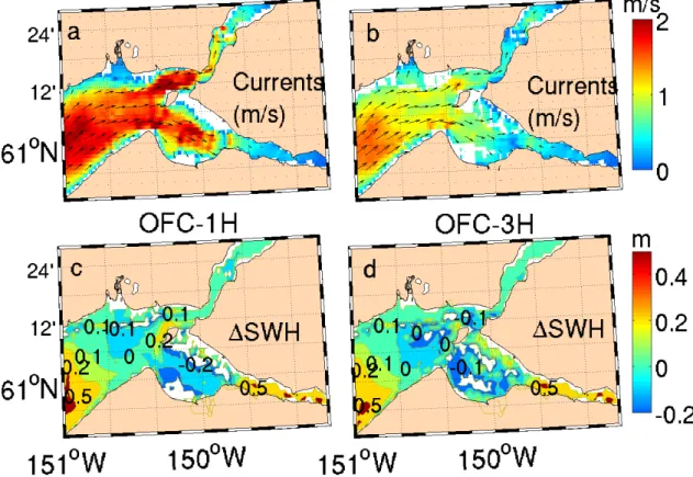
28 Comparison of peak wave period (color) and wave direction (arrows) with (a) no coupling, (b) OFC-1H, (c) OFC-3H during the same time as in Figs. 25-27. . . 55
FIGURE Page 29 Modeled sea-conditions in LCI for the same time as in Fig. 28. (a),(b)
Currents and (c),(d) Difference in SWH with and without coupling for OFC-1H and OFC-3H, respectively. Red elliptical region marks Kachemak Bay area. . . 56 30 Same as Fig. 29 but for upper CI. Note that white spaces denote dry
regions. . . 58 31 Composite map of time-averaged SWHs for the two week period. . . 59 32 Map of time-averaged difference in SWHs with and without the currents
for the two week period. . . 60 33 Map of maximum increase in SWHs at each grid point in presence of
currents for the two week period. . . 61 34 Map of maximum decrease in SWHs at each grid point in presence of
currents for the two week period. . . 62 35 Map showing probabilities of the difference (∆Hs) to exceed a particular
bound, e.g. 10%, 20%, and 30%.. . . 63 36 SWH comparisons of different modeling schemes to data from (a) B05
and (b) B06 for the two-week period. . . 64 37 Energy spectrum comparisons at B05 on 10/26 1800 UTC (during E4).
(a) Measured directional wave spectra, (b,c) modeled directional wave spectra without and with OFC-1H coupling, respectively, and (d) com-parison of 1-D energy spectrum. Arrows in the center of (a)-(c) show wind direction. . . 66 38 SWH comparisons at B05 with and without correction factor to E-W flow. 71 39 Example of adding random noise to input currents. . . 72 40 Maximum increase in modeled SWH (in m) due to addition of random
noise to input currents. . . 74 41 Maximum decrease in modeled SWH (in m) due to addition of random
FIGURE Page
42 SWH comparisons of WW3 output at B78 and B80. . . 76
43 SWH comparisons at B78, B80, and B05 using buoy-imposed spectra. . . 77
44 Energy density (m2/Hz) comparisons. . . . . 78
45 SWH comparisons at B77. . . 79
46 SWH comparisons at B77 with approximated approach.. . . 79
47 Wind comparisons at three weather stations near B05. . . 80
48 SWH comparisons at B05 before and after wind adjustment. . . 81
49 Wind speed comparisons at AUGA2 for (a) Fall 2007 and (b) Fall 2008. Note that only winds blowing from the west were shown. . . 83
50 Maximum increase in modeled SWH (in m) due to addition of random noise to input winds. . . 84
51 Maximum decrease in modeled SWH (in m) due to addition of random noise to input winds. . . 85
52 General location of Kachemak Bay (KB). Red box in the inset shows the geographical location of KB in Cook Inlet, Alaska.. . . 87
53 KB bathymetry in meters. Red diamond shows the location of tidal gauge at Seldovia. . . 90
54 KB domain for coupled wave-current model. . . 91
55 WSE comparisons of KB model with data collected at Seldovia. . . 92
56 Map of “inner” KB showing the extent of dry regions, which are depicted by the green shaded area (source: NOAA). . . 93
57 Sensitivity of modeled dry regions (shown by white spaces) to drying depth. Inset in (a) shows measured (blue line) and modeled (red circle) WSE at Seldovia during the snapshot. . . 94
FIGURE Page 58 Example map of various combinations of tide-, wind-, and river-induced
circulation patterns in KB. “R” in panel c represents location of inflow
in the model. . . 95
59 Intercomparison of modeled SWH for (a) f=0.04-0.5 Hz (25 frequencies), (b) f=0.05-1 Hz (49 frequencies), and (c) difference, (b-a). . . 96
60 Intercomparison of modeled SWH (in m) using low (top panels) and high-resolution (bottom panels) grids for KB region. . . 97
61 Maximum increase in modeled SWH (in m) in presence of currents using finer KB grid. . . 98
62 Maximum decrease in modeled SWH (in m) in presence of currents using finer KB grid. . . 99
63 Prince William Sound domain. Red stars denote the data locations. . . . 101
64 Bathymetry of Prince William Sound. . . 103
65 Satellite tracks over PWS domain. . . 105
66 Influence of (a) global and (b) regional winds on SWHs in PWS. . . 107
67 SWH comparisons using NAM and WRF winds. . . 108
68 An example snapshot of modeled SWH using the outer grid. . . 110
69 SWH comparisons using the outer grid at the locations of (a) buoy 46061, (b) buoy 46060, and (c) buoy 46081. . . 111
70 Inner and outer grids for PWS wave model. . . 112
71 Same as Fig. 68 but for inner grid. . . 112
72 SWH comparisons using the inner (squares) and outer (red circle) grids at the locations of (a) buoy 46061, (b) buoy 46060, and (c) buoy 46081. . 113
FIGURE Page
74 SWH comparisons at the location of buoy 46081. . . 114
75 SWH comparisons for different time-steps. . . 115
76 Snapshot of wind-wave-current conditions for the inner grid. . . 116
77 PWS forecasting system protocol. . . 118
78 SWH comparisons at the location of buoy 46076. Black dashed line repre-sents measured data, alternate red and blue markers depict daily forecasts with 12 h overlap.. . . 122
79 Wind speed (top) and SWH (bottom) comparisons at buoy 46061. Legend is same as for Fig. 78. . . 122
80 SWH comparisons at (a) buoy 46060, (b) buoy 46081, and (c) gauge 410. Legend is same as for Fig. 78. . . 124
81 Spatial comparison of SWH forecast with buoy and satellite data. Colors represent 19-h wave forecast, while numbers in boxes represent measured data. All units are in meters. . . 125
82 Along-track comparisons of wind speed (top) and SWH (bottom) predic-tions. Yellow patch indicates when satellite crossed over land. . . 126
83 Correlation plots of measured and modeled wind speeds (top panels) and SWHs (bottom panels) for (a), (d) L = 9h; (b), (e) L = 19h; and (c), (f) L = 33h.. . . 128
84 Correlation plots of 4-h averaged SWHs for (a) L = 9h, (b) L = 19h, and (c) L = 33h. . . 132
1. INTRODUCTION AND LITERATURE REVIEW
Operational wave forecasts, from a practical standpoint, are critical for safety of maritime operations (e.g. evacuation of oil platforms during storms/hurricanes), planning of coastal and offshore engineering activities (such as installation and main-tenance of offshore structures), and sustainable management of coastal habitat and resources. During the Offshore Wind Energy Workshop (June 2009, Virginia), for instance, it was noted that the installation or operation of offshore wind turbines would be suspended for wind speeds greater than 12 m/s and seas associated with such winds. Wave forecasts are also critical to ship operators (cruise ship accidents caused by waves are well-publicized in the press), as well as to harbor masters respon-sible for securing boats and other equipment in a harbor during foul weather. In the case of oil spills, wave forecasts - in addition to ocean currents - may be needed for spill tracking, containment, and clean-up operations. In some cases, wave-induced surface drift can be of the same order of magnitude as the wind-induced currents that are typically used for predicting spill trajectories.
From a scientific perspective, numerical wave modeling serves as an efficient and cost-effective tool to examine the synoptic patterns of wave generation, propagation, and dissipation over a large spatial domain. In addition, analysis of the model results compared to measured data (if available) provides an estimate of the quality of the output (e.g. wave heights). Such estimates can be used to improve the model, if needed, by appropriate adjustment of the model parameters or by including more complex physical phenomena (wave-current interactions) that were initially excluded.
Furthermore, sensitivity studies of wave predictions to various forcing functions (e.g. winds, currents) help in identifying regions that are most sensitive to input variation and assessing the extent of fluctuation in the model results. For instance, by inducing an artificial adjustment (multiplying by a constant factor or adding random noise) to winds over a spatial region, the wave modeler is able to assess if such a change has any dramatic influence on the output in that region. Mapping of such regions through modeling studies could guide the future deployment of additional data source(s) in those regions. One can establish confidence in models through such data, and also help in understanding the dynamic behavior among various phenomena. Through sequential control of forcing functions in the numerical modeling, the modeler can also identify input forcing(s) that most influence the wave growth (or decay).
The work performed in this dissertation addresses the aforementioned scientific and practical aspects associated with the wave forecasts that have hitherto been only briefly examined. In particular, this dissertation develops the integrated forecasting system for two coastal domains, viz. Cook Inlet (CI) and Prince William Sound (PWS), Alaska by coupling wind, wave, and circulation models. Both these domains present unique challenges such as complex bathymetry, rugged coastlines, sharp to-pographical gradients that influence the wind-fields, significant swell energy from the Gulf of Alaska, and locally generated wind-seas in various channels and inlets. In addition, CI domain experiences strong tidal fluctuations with prominent wetting and drying of shallow areas. Simply put, these processes are complex, dynamic, and inter-twined that render numerical modeling extremely difficult in such domains.
Furthermore, in spite of the famous Exxon Valdez oil spill disaster more than two decades ago, these domains still lack wave information (data as well as reliable model predictions) that is critical for supporting the extensive oil, gas, shipping, fishing, and tourism industries. This dissertation, thus, answers several questions in
order to develop operational wave forecasting systems and fulfill the practical needs associated with various activities noted above. In summary, the main contributions of this dissertation are:
• the development of high-resolution multiscale integrated wave forecasting sche-mes for coastal regions,
• the assessment of the viability of including higher order physics (wave-current interactions), from the viewpoint of efficiency and accuracy, in forecasting schemes that has not been studied in much detail in published literature, • mapping of regions that show significant output variation through model
sen-sitivity studies (as pointed earlier, this could benefit strategic deployment of gauges in the future),
• the development of new techniques for estimating the likelihood of occurrence and uncertainty of a given forecast for use in various practical applications, and
• the development of user-friendly interface for real-time dynamic coupling be-tween wave and circulation models for forecasting purpose (this can be extended to any number or combination of models, e.g. wind, wave, current, sediment transport).
1.1 Historical background
The first evidence of wave predictions can be dated back to the Second World War, when the knowledge of sea-state was required for amphibious assaults in France and North Africa, including the D-day invasion at Normandy. Sverdrup and Munk
(1947) developed wave prediction theory using the wind and wave growth laws to estimate the sea-state, which was also validated using limited data at the time. The work of Pierson et al. (1955) introduced the concept of wave spectrum where the mean wave energy was shown to be distributed along various frequencies and directions, instead of being composed of only a single wave height and period. Gelci and others later described the evolution of wave spectrum using empirical equations (Gelci et al. 1956). Hasselmann (1962) derived a general expression for the source function of wave evolution which was based on three terms representing the wind input, the nonlinear transfer, and the dissipation due to whitecapping. The spectral wave energy equation based on Hasselmann’s work can be described as follows:
DF(f, θ)
Dt =Sin+Snl +Sds (1)
whereF is the mean wave energy spectrum,f is the wave frequency, andθis the wave propagation direction. The left hand side of Eq.(1) represents the linear propagation of wave energy in space, whereas the right hand side is composed of the source and sink terms identified by Hasselmann. Sin describes the wave growth due to
wind input (source term), Snl describes the nonlinear wave-wave interactions, and
Sds is the dissipation term due to whitecapping (sink term); these terms are also
dependent uponf,θ. The above equation is still being used in different forms today, most notably for the coastal waters where other nonlinear phenomena also affect the wave energy spectrum (discussed later).
A major breakthrough in understanding the evolution of wave spectra was made through the Joint North Sea Wave Project (JONSWAP; Hasselmann et al. 1973). Contrary to the Pierson-Moskowitz spectrum (Pierson and Moskowitz 1964), which showed that the waves become fully developed after wind blows steadily for a long
duration, Hasselmann et al. (1973) found that the wave spectrum is never fully developed and rather continues to evolve in space and time through nonlinear wave-wave interactions.
In the mid to late 1970s, with the availability of faster computers, advance-ments to numerical wave predictions began to take shape. During the SWAMP study (SWAMP 1985), wave models were distinguished between the first generation (1G) and second generation (2G) type. 1G models neglected the nonlinear wave interactions, while the 2G models included such interactions in an empirical man-ner. Through various modeling tests, SWAMP study compared the performance of 1G and 2G models and found the results from the two models to be comparable. However for one test simulating the wind conditions during a hurricane, the mod-els produced wave heights that differed significantly. It was then determined that the two-dimensional description of sea-state was more important than simply using parametric models. This finding led to the development of a full spectral model that provided full two-dimensional description of the sea-state. The full spectral model was classified as the third generation (3G) wave model. The 3G model explicitly ac-counts for the nonlinear wave interaction term (Snl in Eq.1) and the spectral shape
is allowed to develop dynamically without any constraints.
Modeling the sea-state using 3G models has become more efficient through ad-vances in computing power and numerical schemes. The wave model (WAM) was the first 3G model (WAMDIG 1988; Komen et al. 1994) and solved the action bal-ance equation of the form similar to Eq.(1). Since WAM, a number of other wave models have been developed such as WAVEWATCH III (hereafter WW3; Tolman 1991, 1999, 2009), Simulating Waves Nearshore (hereafter SWAN; Booij et al. 1999, Ris et al. 1999), etc. All these models belong to the 3G type and solve the full
two-dimensional spectrum of the sea-state. In addition, these models have been used for wave hindcasting and forecasting throughout the world (details in the next section).
1.2 Overview of operational forecasting
Operational forecasting for offshore regions has been undertaken through the ef-forts of various meteorological offices such as the European Centre for Medium-Range Weather Forecasting (UK) or the National Oceanic and Atmospheric Administration (NOAA; USA) which have been providing, for several years, continuous forecasts of oceanic conditions (wind velocity, significant wave height (SWH), peak wave period (Tp), peak wave direction (Dp), etc.); these forecasts contribute to various
engineer-ing operations includengineer-ing, for example, the evacuation of oil platforms in advance of hurricanes in the Gulf of Mexico. As a result of these developments, the fundamental viability of the approach and the basic protocols for producing such forecasts have been established; various NWS offices (Eureka, Anchorage, Dickinson, etc.) and the public appear to be using the products. The results of the data suggest that (i) it is reasonable to expand such efforts to new regions where a demand for local ocean weather information exists, and (ii) it is necessary to address certain limita-tions encountered in present efforts (the “first generation” of coastal wave forecasting schemes), or in other words, to advance the technology through more sophisticated model implementation procedures in order to gain improved reliability.
In the US, NOAA’s National Centers for Environmental Prediction (NCEP) uses the well established third-generation wave model WW3 which primarily incorporates formulations for wave generation, dissipation, and nonlinear wave-wave interactions. NCEP’s modeling efforts encompass the entire globe at a coarse resolution (∼30 km) and provide forecasts for upto 7 days in advance. NCEP’s forecasts, however, do not
extend into nearshore domains, primarily because in such regions other small-scale nonlinear phenomena exist that are not properly accounted for in the global version of WW3. Recently, a shallow water version of WW3 (version 3.14) became available that incorporates shallow water processes such as triad wave-wave interactions, bot-tom effects, and depth-induced wave breaking. NCEP uses the shallow water version of WW3 for the coastal regions of the US and generates forecasts on a multi-grid setup with better resolved grids. For example, in Alaskan waters, wave forecasts are generated on regional (∼ 15 km) and coastal (∼ 7 km) grids. Nevertheless, these resolutions are still not fine enough to resolve the rugged and whimsical coastal do-mains present throughout the US (e.g. Mobile Bay, Alabama; Corpus Christi, Texas; Gulf of Maine, Maine; Cook Inlet (CI) and Prince William Sound (PWS), Alaska; etc.). Furthermore, other higher order effects (such as those induced by the presence of currents, changing water levels, etc.) are still not part of NCEP’s ongoing efforts and the role of such effects on the forecast efficiency and accuracy is not fully known. One simple solution is to accommodate the effects of high-resolution local ge-ometries and relevant physics (e.g. wave-current interaction) in regional models that interface with the NCEP’s outer ocean forecasts, thus enabling the extension of NCEP’s products into coastal regions at the appropriate scales. In recent years, coastal forecasting systems such as the Gulf of Maine Ocean Observing System (GO-MOOS), the Alaska Ocean Observing System (AOOS), etc. which involve bay-scale domains coupled to the outer ocean forecasts have gained prominence. To account for the effect of tides and currents on the waves, the wave model is coupled with an appropriate circulation model. For instance, wave forecasts in Humboldt Bay (provided by National Weather Service, Eureka) include the effect of tidal currents near the harbor entrance. Coupled forecasts of surface waves and currents are also provided by the Naval Research Laboratory for the Mississippi and Southern
Cali-fornia Bights. It is to be noted that although such systems exist, these are developed for domains that do not present complex challenges such as those found in CI and PWS. In particular, the tidal range and magnitude of the currents at these locations are not as extreme compared to those found in CI. In addition, the reliability and uncertainty of these systems has not been addressed in published literature.
Some other examples of forecasted metocean conditions include coastal currents in Galveston and Matagorda Bays (provided by the Texas Water Development Board http://midgewater.twdb.state.tx.us/bays˙estuaries/bhydpage.html), Penobscot Bay (www.gomoos.com); and wave conditions in Humboldt Bay (http://www.wrh.noaa. gov/eka/swan/), in the Great Lakes (provided by NOAA; http://www.glerl.noaa.go-v/res/glcfs/), and in Penobscot and Massachusetts bays (www.gomoos.com).
1.3 Literature review
Several near-shore models, such as STWAVE, MIKE21, SWAN, WW3 v3.14, account for shallow water processes such as triad wave-wave interactions, dissipation due to bottom friction and depth-induced wave breaking (Booij et al. 1999; Ris et al. 1999; Sorensen et al. 2004; Tolman 2009) and can be used to extend the offshore wave climatology into near-shore areas. Notably, the wave model SWAN has received considerable attention for application in the coupled mode (note that “coupled” mode in this instance refers to coupling between a global and a local/regional wave model and not the coupling between a wave model and a circulation model) for engineering studies. For instance, Millar et al. (2007) coupled the coarse-resolution global simulations to a regional SWAN domain to examine the impacts of wave energy farms off the UK coast. However, their local simulations were performed for specific (a series of individual) wave events, in a “stationary” mode with zero wind imposed
on the local grid. The inclusion of local winds was described by Rogers et al. (2007) for studies in Southern California Bight using multiple levels of grid coupling; again, however, the stationary mode was invoked, about which they acknowledge: “Use of stationary assumption for a large computational region can lead to poor timing of swell arrivals and temporal description of local growth and decay”. They also state: “the stationary assumption implies instantaneous wave propagation across the domain, as well as instantaneous wave response to changes in the wind field”. It is to be noted that in addition to these simplifications which could adversely impact predictions, these studies primarily involved hindcasts, as did the unsteady-state six-and-a-half years of coupled simulations performed by Panchang et al. (2008) for aquaculture engineering and other applications in coastal Maine. Some other studies that have tested various aspects of SWAN (some with multiple levels of nesting) in the hindcast mode include applications on the open coast (e.g. Rogers et al. (2003) in Mississippi Bight; Zubier et al. (2003) in Duck, NC) as well as those in semi-enclosed areas (e.g. Gorman and Nielsen (1999) in Manukau Harbor; Chen et al. (2005) in Mobile Bay; Moeini and Etemad-Shahidi (2007) in Lake Erie; Panchang et al. (2008) in Penobscot Bay). In contrast, studies related to the evaluation of SWAN in the forecast mode are scarce (e.g. Rogers et al. (2007) in Southern California Bight; Allard et al. (2008) in Portugal; Dykes et al. (2009) in the Adriatic Sea).
Although the viability of interconnecting regional wave models to global coun-terparts is well established, the impact of other higher order effects (wave-current interaction, wetting and drying, etc.) on regional wave models is still poorly under-stood. To account for such phenomena, the wave model has to be coupled to an appropriate circulation model. There are several theoretical as well as experimental studies that have addressed the effects of wave-current interaction, e.g. Huang et al. (1972), Thomas (1981), Nwogu (1993), Hedges et al. (1985), Chakraborti (1996),
Guedes Soares and de Pablo (2006), etc. However, only a few studies have been undertaken for real-life applications. These include studies of Chen et al. (2007) and Funakoshi et al. (2008), who coupled SWAN and ADCIRC (“Advanced Circu-lation”) for various applications in Mobile Bay and Florida, respectively. However, the intensity of currents in these studies was rather small (∼ 0.5 m/s) compared to those found in CI (∼ 2.5-3 m/s). Further, both studies were done in the hindcast mode where computational efficiency was not an issue. In the forecasting mode, on the other hand, efficiency becomes a critical consideration so that the output can be provided in reasonable time.
1.3.1 Hindcast vs. forecast
In engineering applications, simulations in the hindcast mode are usually lim-ited in scope: they are performed for a set of predetermined specific events. These simulations can be repeated after modifying or adjusting various model parameters or forcing functions, using available data as a guide, and the best possible spa-tial/temporal resolution can be used. Simulations in the forecast mode, on the other hand, offer the modeler relatively little flexibility in this regard. The modeler has no data for the future and has little recourse (except data assimilation) if the forecast indicates a mismatch with the data (if available). Model resolution may be dictated to a greater extent by the logistics of obtaining a forecast rather than by modeling accuracy. Forcing functions also may contain inaccuracies, against which there may be no easy remedy. Thus, once a system has been designed (guided by hindcast studies), the modeler has little choice but to accept the flaws of the system. There-fore, a specific assessment of the forecast skill must be provided. This will enable the manager of engineering operations to invest the appropriate confidence in the
forecast and plan accordingly. Indeed, companies providing met-ocean services are sometimes penalized if their predictions turn out to be faulty.
To address forecast uncertainty, forecast centers sometimes run wave model en-sembles. This issue has also been recently addressed in a limited manner by Bidlot et al. (2002) for global simulations (not regional) and Dykes et al. (2009) for the Adriatic. These studies compared model predictions to data. However, the compar-isons are provided in the form of the usual statistics (viz. correlation coefficients, best-fit slopes, scatter indices etc.) which do not, on their own, assist the manager of engineering operations in establishing the likelihood of occurrence of a predicted condition. In contrast, one of most significant contributions of this dissertation is the provision of forecast uncertainty to the end-user (in addition to the usual statistics).
1.4 Research objectives
To be more specific, the goals of this study are to develop integrated forecasting schemes and examine the issues noted above for coastal regions where accurate wave information is needed for a variety of coastal and offshore operations. Specifically, the forecasting schemes developed in this dissertation are tested for CI and PWS (Fig.1) domains. Even after more than two decades of the historic Exxon Valdez disaster, these regions suffer from a lack of accurate wave information. In addition, due to existing and ever expanding offshore engineering, there is an established need for ocean weather predictions in these regions. Numerous cargo ships, oil tankers, fishing, and recreational vessels traverse PWS and CI round the year.
As discussed earlier, from the technical/modeling perspective, the PWS and CI domains are characterized by extremely complex geometry, a larger overall size than most domains on which such programs have been implemented, islands and
moun-Fig. 1. Cook Inlet and Prince William Sound domains.
tainous terrains that influence the wind-fields, and strong tidal effects. It is therefore necessary to use a combination of wind, wave, and circulation models. There are sev-eral candidate models that can be utilized for such coupled studies. SWAN is the most suitable option for performing wave simulations in unsteady state. As for the circulation modeling, both finite element type (ADCIRC) and finite difference type (ROMS, POM, EFDC) models could be used. All these models have various capabil-ities and have been evaluated for numerous cases. In particular, EFDC (“Environ-mental Fluid Dynamics Code”) is the most diverse and advanced three-dimensional model that internally links the hydrodynamic, sediment transport, water quality and eutrophication, and toxic contaminant transport (e.g. oil spill) submodels in a single source code (Hamrick 1992). Thus, EFDC has great advantage over other models in terms of eliminating the need for complex interfacing of multiple models to ad-dress the different processes. In this dissertation, SWAN and EFDC were chosen for
wave and circulation modeling, respectively (details of the two models are given in Sections 2.1-2.3).
In particular, this dissertation addresses the adequacy of the circulation model and the level of wave-current interaction required to obtain appropriate forecasts in CI and PWS. A detailed qualitative assessment of coupled model predictions is also performed to determine regions which show prominent wave-current interactions. Due to paucity of observations in CI domain, quantitative comparisons, to the extent possible, are also made to assess the reliability of predictions in CI. In particular, the development of the CI integrated forecasting scheme is guided by a two-week period which consisted four distinct storm events with wave heights ∼ 5m. Sensitivity analysis is also performed to identify the sources of errors in the wave predictions and to map regions where such errors are large. Such analysis would eventually serve as “guidance” for estimating the modeling uncertainty of the forecasts, especially in CI region where no reliable information currently exists.
As for the PWS domain, more comprehensive datasets are available for estimating model veracity. Specifically, data from four buoys, two wave gauges, and three satellites are available, which greatly benefit the estimation of uncertainty of the model forecasts. Thus in this dissertation, the reliability assessment is done for about a year of wave predictions (June 2007 to May 2008) for PWS domain. This analysis provides the estimates of likelihood of occurrence of a given forecast (in addition to the usual statistics), which can be used by managers of engineering operations, who are ultimately interested in knowing the likelihood of a predicted condition to actually occur and the associated error bounds.
The dissertation is organized as follows. Section 2 provides an overview of the wave and circulation models and their governing equations. Section 3 describes the development of the integrated forecasting scheme for CI, followed by rigorous
sensi-tivity analysis to study the impact of various forcing functions on wave predictions in Section 4. Results of Sections 3 and 4 motivate the study in Kachemak Bay (Sec-tion 5) to further study the effects of wave-current interac(Sec-tion on high-resolu(Sec-tion grids. The focus is then shifted to PWS and the development of PWS forecasting system is first described in Section 6. This is followed by reliability assessment of the PWS forecasts in Section 7. Summary, conclusions, and directions for future work in Section 8 conclude this dissertation.
2. OVERVIEW OF WAVE AND CIRCULATION MODELS
2.1 Wave model
For simulating the wave-field, the wave model SWAN (“Simulating Waves Near-shore”) was utilized. SWAN is a third-generation (since non-linear interactions are explicitly accounted for, see Section 1.1) spectral wave energy model capable of simulating wave propagation in time and space, shoaling, refraction, blocking, and reflection due to spatial variations in bathymetry and currents (Booij et al. 1999, Ris et al. 1999, Holthuijsen 2007).
In general, the wave models determine the evolution of action densityN in space and time, rather than the energy density E. This is because in the presence of ambient current, the action density is conserved while the energy density is not. The action density is related to energy density by the expression N = E/σ, where σ is the relative wave frequency. The governing equation in SWAN model is thus based on the following spectral action balance in spherical coordinates:
∂N ∂t + ∂cλN ∂λ + (cosϕ) −1∂cϕcosϕN ∂ϕ + ∂cθN ∂θ + ∂cσN ∂σ = Stot σ (2)
where N is the action density, λ and ϕ denote the geographical space coordinates (longitude and latitude, respectively), θ is the wave propagation direction (θ and σ denote the spectral space coordinates), andStotis the total source/sink term (similar
to Eq. 1) that describes the wave growth due to wind input, nonlinear wave-wave interactions, and dissipation due to whitecapping, depth-induced wave breaking, and bottom friction.
The first term on the left-hand side of Eq. (2) represents the time rate of change of action density, the second and third terms represent the propagation of action density in geographical space with velocities cλ and cϕ. The propagation velocities
are given by the expressions cλ = (cgcosθ+uλ)/(Rcosϕ) and cϕ = (cgsinθ+uϕ)/R,
where R is the radius of the earth, uλ and uϕ are the depth-integrated ambient
current velocities in longitudinal and latitudinal directions, respectively. The fourth term represents depth-induced and current-induced refraction, while the fifth term represents frequency shift due to variations in depths and currents. cθ and cσ
rep-resent propagation velocities in the spectral space. The group velocity cg =∂σ/∂k
follows from the dispersion relation σ =qgktanh(kh) wherek is the wave number, and h is the water depth.
Note that Eq. (2) reduces to the energy balance equation in the absence of currents (the fifth term on left hand side of Eq. 2 disappears since there is no frequency shifting).
The SWAN model solves the above action balance equation using implicit solution schemes that are unconditionally stable (i.e. not dependent upon Courant-Friedrichs-Lewy criterion). Such schemes permit the use of finer grid resolutions without com-promising the computational efficiency, which makes SWAN the appropriate choice for modeling studies undertaken in this dissertation.
2.2 Circulation model
This dissertation makes use of EPA’s EFDC model (Hamrick 1992) for simulating barotropic circulation in the selected coastal domains. EFDC is capable of simulating three-dimensional flow, transport, and biogeochemical processes in surface water systems such as rivers, estuaries, lakes, reservoirs, and coastal regions. The EFDC
model has been extensively tested and documented in a wide range of environmental and hydrodynamic studies (Kuo et al. 1996; Shen et al. 1999; Shen and Kuo 1999; Ji et al. 2001; Jin et al. 2001; Jin and Ji 2001, 2005; Park et al. 2005; Zou et al. 2006), and is being used by several universities, national laboratories, government agencies, and other private firms.
EFDC solves the three-dimensional, vertically hydrostatic, free surface, turbulent averaged equations of motion for a variable density fluid. The model uses a sigma vertical coordinate and cartesian or curvilinear, orthogonal horizontal coordinates. The model also incorporates the Mellor-Yamada level 2.5 turbulence closure scheme (Mellor and Yamada 1982) to explicitly solve for the vertical eddy viscosities in equations of motion. The model also has the capability to account for wetting and drying of shallow areas (Ji et al. 2001), which is of significance in CI domain given the large tidal fluctuations.
The generalized equations of EFDC with the horizontal curvilinear coordinates and the sigma vertical coordinate for the conservation of momentum and continuity are given by:
(3) ∂t(mHu) +∂x(myHuu) +∂y(mxHvu) +∂z(mwu)−mf Hv
=−myH∂x(p+gη)−my(∂xh−z∂xH)∂zp+∂z(m Av H∂zu) +Qu (4) ∂t(mHv) +∂x(myHuv) +∂y(mxHvv) +∂z(mwv)−mf Hu =−mxH∂y(p+gη)−mx(∂yh−z∂yH)∂zp+∂z(m Av H∂zv) +Qv (5) ∂t(mH) +∂x(myHu) +∂y(mxHv) +∂z(mxmyw) =QH
where x and y are the curvilinear-orthogonal coordinates, z is the vertical sigma coordinate, uandv are the horizontal velocity components, wis the vertical velocity
in the sigma coordinate, mx andmy are the metric coefficients for curvilinear system
and m =mxmy is the Jacobian (if mx =my = 1, the system becomes cartesian).
Eqs. (3), (4) represent the horizontal momentum conservation where H is the total depth (=h+η), with h being the depth below the surface (z = 0), and η the surface undulations around z = 0 (could be negative or positive). f is the coriolis parameter, Av is the vertical eddy viscosity, p is the pressure term, Qu and Qv
represent the momentum source/sink terms (e.g. wind stress, momentum diffusion). Eq. (5) represents the continuity equation. QH is the source/sink term that takes
into account the freshwater discharge through rivers, precipitation, evaporation, and other sources. Note that the vertical momentum equation is based on the hydrostatic assumption, which relates vertical pressure gradient to the product of water density and gravity.
The equations (3)-(5) will form a closed system for the variables u, v, w, p and η, if the vertical turbulent viscosity (Av) and the source/sink terms (Qu, Qv, and
QH) are explicitly specified. The vertical turbulent viscosity is provided through the
model developed by Mellor and Yamada (1982), which is based on a pair of transport equations for the turbulence intensity and length scale, and is computed internally in EFDC.
2.3 Background on wave-current interaction
When the waves encounter the currents and vice-versa, the excess momentum flux induces a net transfer of energy between the waves and the currents. As a result, the interaction alters both the waves and the currents.
2.3.1 Effect of currents on waves
Currents can affect the waves by changing the wavelength (or wave heights) and/or through refraction effects as waves propagate over a current. The changes in the wavelength depend upon the magnitude of the current speed and the angle between the wave propagation and current direction. In general, when waves and currents are in the same direction, the wavelength increases (wave height decreases and hence wave steepness - ratio of wave height/wavelength - decreases). In contrast, when the waves oppose the currents, wavelength decreases (wave heights increase and so does steepness). The equation relating the currents to the waves is given by
ω =σ+−→k .−→U (6)
where ω is the absolute angular frequency, σ is the relative angular frequency, −→k is the wave number vector, and −→U is the current velocity vector. This equation, in general, refers to the Doppler shift.
In SWAN, if ambient currents are present (e.g. output from a circulation model), then the iteration scheme solves for the action density propagation due to the shift in frequency (i.e. fifth term on left-hand side of Eq. 2 is accounted) through the use of relation in Eq. 6. As noted earlier, if ambient currents are not included, then the frequency shift term drops out from Eq. 2 and the governing equation reduces to the energy balance type.
2.3.2 Effect of waves on currents
Wave motion can also affect the waves through gradients of radiation stress (Longuet-Higgins and Stewart, 1964). Radiation stress usually refers to the mean
excess momentum flux due to the presence of the waves. Variations in radiation stresses (i.e. the gradients) play an important role in understanding various coastal processes such as wave setup and setdown, wave-current interaction, and longshore current in the surf zone that affects the sediment transport.
SWAN, at present, does not compute wave-induced currents and thus these cur-rents, if relevant, have to be included as a component while evaluating the current-field through the use of a circulation model. Similar to the wind stress, the circulation models simulate the wave-effects on currents through the gradients of radiation stress. This extra source term is added to the right-hand side of the horizontal momentum equations (usually a part of Qu and Qv in Eqs. 3, 4).
The equations for the gradients of the radiation stress are usually given by
Fx =−
∂Sxx
∂x − ∂Sxy
∂y (7)
in the x-direction, and
Fy =−
∂Sxy
∂x − ∂Syy
∂y (8)
in the y-direction, whereSxx,Syy, andSxy are the components of the radiation stress
tensor S. For a plane progressive wave propagating at an angle θ, these components can be expressed as:
Sxx = " (1 + cos2θ) kh sinh 2kh+ 1 2cos 2θ # E (9) Sxy = kh 2 sinh 2kh + 1 4 ! Esin(2θ) (10)
Syy = " (1 + sin2θ) kd sinh 2kh + 1 2sin 2θ # E (11)
whereh is the water depth, k is the wave number, andE is the wave energy. SWAN provides the output of gradients of radiation stress (Fx and Fy through eqs. 7-8),
that could be used as input forcing in the circulation model to account for the wave-induced currents. EFDC, however, does not accept gradients of radiation stress directly. In particular, EFDC requires a radiation stress tensor (i.e. eqs. 9-11) and computes the gradients of radiation stress internally in the code. In addition, EFDC only accounts for the steady-state radiation stress forcing. SWAN, at present, does not have an option to output the radiation stress tensor.
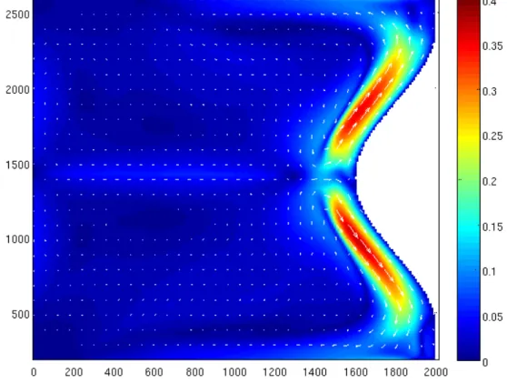
To solve these issues, a separate code wrapper was built in EFDC that bypassed the requirement of radiation stress tensor. Essentially, the “unsteady” gradients of radiation stress from SWAN were directly embedded through this wrapper into EFDC. This forcing term was then added to the right-hand side of horizontal mo-mentum equations of EFDC (Eqs. 3-4).
The updated EFDC code was tested for Dingemans case (Dingemans et al. 1987), that predicted wave-induced currents around a coastline with cosine-squared protu-berance and rather straight bottom contours (both generated through formulas given in Dingemans paper). SWAN was forced by a single wave on the open boundaries, propagating in the +x-direction with wave height 1 m and period 8 s. SWAN-computed gradients of radiation stress were then fed into EFDC through the updated code wrapper. Fig. 2 shows the EFDC-modeled wave-induced currents for Dinge-mans test case. These results closely match those obtained by DingeDinge-mans (Fig. 10 of Dingemans et al. 1987). This exercise shows that the updated version of EFDC works well for simulating wave-induced currents.
Fig. 2. Wave-induced currents (in m/sec) from EFDC using code wrapper for gra-dients of radiation stress.
3. DEVELOPMENT OF INTEGRATED WAVE FORECASTING SCHEME FOR COOK INLET, ALASKA
3.1 Introduction
Cook Inlet (CI) is a large estuary (∼180 miles long), stretching from the Gulf of Alaska to Anchorage in south-central Alaska (Fig. 3) and experiences a great deal of human activity (such as shipping, oil and gas extraction, etc). Approximately half of Alaska’s population lives along CI’s shores. Anchorage, between Turnagain and Knik Arms at the head of CI, is Alaska’s largest city and a center of trans-portation, commerce, industry, and tourism. The Port of Anchorage receives food, fuel, building materials, durable and expendable supplies for delivery to over 80% of Alaska’s population and to four large military installations; while seafood, minerals, and gas are exported. Shipping routes in CI serve the port year-round, as well as the ports of Nikiski, Homer, and Drift River with transshipment to smaller coastal communities. Other marine traffic is related to the recreation and tourism industries as well as commercial fishing. Homer Harbor is one of the largest boat harbors in the state and accommodates commercial and charter fishing, excursion, government agency, and private recreation boats. The majority of citizens living in south-central Alaska rely on the marine environment to some extent for subsistence, recreation, or commerce.
CI is also an extremely dynamic system. Being exposed on three sides to the Gulf of Alaska, which has among the largest waves in the world, the activities noted above can be subject to complex and dangerous surface wave action. A cursory examination of the brief dataset available from Buoy 46105 (hereafter, B05), near Stevenson Passage, suggests that significant wave heights (SWHs) can be as large
Fig. 3. Cook Inlet domain.
as 7 m (corresponding to “maximum” wave conditions of about 13 m in that sea-state). There are also large tidal variations (about 8-9 m, the largest in the US) and the complex bathymetry and coastal morphology result in large tidal currents. For example, tidal bores are commonly found in Turnagain Arm, creating currents in excess of 2-3 m/s. Currents on the order of 1-2 m/s also occur throughout the inlet during full tidal flow. There is also significant wave/current action and during low tide, silty bottoms (mudflats) are exposed which compound navigation difficulties. The Anchorage Daily News has often publicized grounding of boats during low tide. In addition, the interaction of rugged topography (mountain ranges with elevations that abruptly rise to 3000 m, gaps, and channels) with the strong atmospheric pres-sure gradients results in the so-called “gap winds” that adversely affect maritime and aviation activities during the winter season (Liu et al. 2006). Also important is the
impact of the strong tidal flows through lower CI into and out of the Gulf of Alaska. Mariners piloting vessels in the region attest to the impact of the interaction of these forces on maritime operations. Given the paucity of wave observations in CI, it is critical to provide accurate and timely forecasts of surface conditions through the use of state-of-the-art wave/circulation models.
Over the last few years, several regional wave forecasting systems have been established for various locations around the US. As discussed in Section 1.2, these systems provide wave forecasts on high-resolution grids and are connected to NCEP’s coarse resolution global wave forecasts (Tolman 2009). In some cases, the regional wave model is also coupled with the circulation model to account for wave-current interaction (Chen et al. 2007, Funakoshi et al. 2008).
The viability of interconnecting multiple models (i.e. winds, waves, and cur-rents) in dynamic environment such as CI presents unique challenges that have hith-erto been only briefly examined. The sharp topographic gradients produce complex wind regimes that should be properly modeled, in order to obtain reliable simula-tions of waves and currents. The strong currents noted earlier, which are created by winds, tides, and other (e.g. baroclinic forcing) mechanisms, can influence the waves (a strong opposing current could increase the wave height and steepness). Waves, in turn, could also affect the currents by transferring their momentum to currents through gradients of radiation stress (Longuet-Higgins and Stewart 1964). This dynamic feedback between the waves and the currents, and its effect on surface conditions should thus be addressed in CI wave modeling. The interest of this study is to include those phenomena in regional forecasting schemes that may indeed af-fect the waves, but without expanding the cost and effort required to generate the forecast.
This section describes the development of an integrated wave model that includes the complex effects induced by winds, currents, and water-levels in CI. Wave-current interaction is studied by one- and two-way coupling of the wave and circulation models, using a two-week period in October 2008 that included multiple storm events with winds in excess of 20 m/s and SWHs about 4-6 m in lower CI. Such events are potentially hazardous to mariners and fishermen operating in the region. SWAN and EFDC were chosen for wave and circulation modeling, respectively. In particular, this study addresses the adequacy of the circulation model and the level of wave-current interaction (one-way or two-way) required to obtain appropriate forecasts. The influence of the time interval for information exchange between the two models on the results and on modeling efficiency is also addressed. A detailed qualitative and quantitative assessment of coupled model predictions is also performed to determine regions which show prominent wave-current interactions. Spatial maps showing the extreme SWH variation in the presence of currents are also created for use in various applications.
This section is organized as follows: Section 3.2 provides a description of various bathymetric datasets available, along with a qualitative assessment of bathymetric patterns in the CI region. Section 3.3 describes the surface-wind models available for use in the wave and circulation modeling schemes, followed by Section 3.4 that addresses the development of a basic circulation model, run in the barotropic mode (with tides, winds, and river discharge), for wave forecasting purposes. The adequacy of the barotropic model is also addressed by comparison with flow measurements in various parts of the CI domain. Section 3.5 describes the development of a gen-eral wave model for CI, followed by Section 3.6 that describes the coupling options suitable for wave-current interaction studies, along with the coupling procedure.
Sec-tion 3.7 describes the applicaSec-tion of coupled modeling system to four storm events, followed by discussion in Section 3.8.
3.2 Bathymetric information and available datasets
Bathymetry is one of the most critical aspects regarding the performance of any coastal model. Plant et al. (2009) showed the influence of bathymetric filtering on wave and flow fields, and found that the model results were extremely sensitive to the resolution of input bathymetry.
NOAA’s National Geophysical Data Center provides various bathymetric datasets for CI such as Etopo1/Etopo2 Global Relief Models, Tsunami Inundation Digital Elevation Model (DEM; NOAA Center for Tsunami Research), etc. The Etopo datasets have a fairly low resolution (1 min and 2 min) and do not properly resolve many complex bathymetric features of CI, while the DEM dataset is available at a 24 sec resolution, presently the highest resolution available for CI region.
Although the DEM is the best available resolution for CI domain, the Turnagain arm region of upper CI is not properly resolved. In the entire arm, the depths are set to 3 cm (due to missing data) which may be inappropriate to simulate the wetting and drying of the region. To compensate for the missing bathymetry, past NOS surveys (conducted between 1900-1939) were utilized along with the navigational charts in the Turnagain Arm region. These data were interpolated onto the existing DEM to generate a more reliable bathymetry (a similar approach was used by Oey et al. 2007). The updated bathymetry is shown in Fig. 4. In general, the depths decrease from about 200 m near Stevenson Passage (in the south) to about 50 m in the central inlet. The depths also show across-shore variability in various regions
Fig. 4. Bathymetry of Cook Inlet (in meters).
(e.g. near Kalgin Island), with depths reducing from greater than 50 m to less than 10 m. Overall, CI is mostly shallow with an average depth of about 50 m.
3.3 Surface weather patterns
CI experiences very complex and dynamic weather patterns. During the winter season, winds in the northern Gulf of Alaska are a result of cyclonic storm systems off the Pacific and attain maximum strength from October through March (Stabeno et al. 2004). Due to the presence of Chugach Mountains (spanning the entire CI coastline), these storms linger and funnel down through various gaps and channels resulting into random and complex wind regime (Liu et al. 2006). It is critical to reliably model such complex weather patterns for forecasting purposes, since it is
frequently stated that the quality of wave model predictions are most dependent on the quality of the input winds (Dykes et al. 2009). Unfortunately, there are not many weather stations that provide a synoptic snapshot of wind patterns over the entire CI. For example, the northern CI (north of the Forelands) only has one weather station near Anchorage that was installed by the NOS in April 2005, which provides real-time measurements of wind and gust speed, wind direction, air temperature and pressure every six minutes. Elsewhere, there are a total of six active weather stations, but these are too few to obtain a reliable description of weather patterns over this region (Fig. 5).
Fig. 5. Locations of weather stations in CI domain.
Over the last few years, NCEP’s NAM (“North-American Mesoscale”) model has provided a synoptic snapshot of surface winds over the global ocean, which are
assimilated through satellite-based measurements to improve their reliability. How-ever, the NAM winds do not properly account for coastal topographical variations, their resolution is much too coarse, and often these winds do not extend into several coastal domains (e.g CI, PWS, etc.). As an example, Fig. 6 shows a sample plot of predicted winds using NCEP’s NAM model at a resolution of about 7 km. It can be clearly seen that the NAM model does not appropriately resolve the wind-fields near the coastlines and also does not extend inside the PWS domain, and hence may have adverse implications to nearshore wave and circulation modeling.
Fig. 6. Sample plot of NCEP predicted winds over northern Gulf of Alaska. Color represents wind speed (in meters/sec), whereas arrows depict wind direction.
Since early 2007, operational weather forecasts using the WRF (“Weather Re-search and Forecasting”) model have become available (http://aeff.uaf.alaska.edu/). These provide better coverage of the CI domain and use resolutions fine enough
to resolve the salient features of the underlying topography. WRF is also the latest mesoscale model adopted by the National Weather Service as well as the U.S. military and other meteorological services for generating high resolution weather forecasts in various coastal regions. The WRF model performance has been documented in sev-eral studies (e.g. Done et al. 2004; Kain et al. 2006; M¨olders 2008). Details of the model and its performance are discussed elsewhere (Olsson and Volz 2011; M¨olders et al. 2008). While there are some errors in the predictions (described later), Singhal et al. (2010) found their effect on wave predictions to be marginal. A sample plot of WRF predicted winds is shown in Fig. 7, and being on a higher resolution, it ex-tends into nearshore domains. This dissertation thus uses the WRF winds obtained through the link noted above for wave modeling in CI.
3.4 Surface-current patterns and modeling
Circulation in CI is mostly tidally-driven with tidal period predominantly due to the M2 tidal constituent. The natural resonant frequency of CI is roughly equivalent to that of the tidal frequency, and as a result CI experiences one of the largest tidal fluctuations in the world. In addition to tidal forcing, wind-driven and buoyancy-driven flows also contribute to the overall circulation patterns in CI (Okkonen and Howell, 2003, Okkonen et al. 2009). Tidal and baroclinic effects were also addressed in modeling studies by Oey et al. (2007) and Johnson (2008). While these studies have addressed the circulation patterns and their seasonality in CI, how these affect the wave climate in general has yet to be understood. Thus, the emphasis here is on the development of a base circulation model that is capable of simulating the barotropic circulation (wind, tide, and river discharge). The output of the circulation model (i.e. surface-currents/water levels) will be used as input to the wave model. The goals are to 1) address the adequacy of the barotropic model, 2) understand the effects of wave-current interaction on overall wave climate in CI, and 3) examine the impact of adding currents/water-levels in the wave model from the viewpoint of efficiency of the forecasts.
For barotropic modeling, the EFDC model is utilized. The model was applied to the CI domain covering the region between -156 W to -149 W and 56 N to 61.5 N, on an irregular grid with a resolution of about 4 km at the open ocean boundaries, and decreasing to a resolution of ∼1.5 km in the northern-most parts of CI (Fig. 8). Other model resolutions were also tested (e.g. <1 km) for this domain, however the model simulation time increased drastically for higher resolutions without a major impact on the accuracy of the results. Since the goal is to transition the modeling into
real-time operational mode, some compromise regarding the model grid resolution is needed in order to make efficient, yet accurate, forecasts.
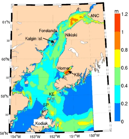
Fig. 8. Circulation model domain (red dashed line) along with data measurement locations. Blue circles represent current measurement locations, red stars represent wave buoys, and green triangles represent tidal gauges.
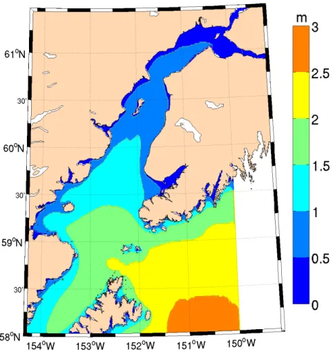
The CI circulation model was tested via the simulation of tidal conditions for the summer of 2005 (May-August). This period was selected mainly because it co-incided with NOAA’s comprehensive field campaign of current measurements within CI. Ten locations were selected from this survey for model comparison (current me-ter locations are shown in Fig. 8). Modeled wame-ter surface elevations (WSEs) are
also compared with data from four tidal gauges (locations shown in Fig. 8). The model was initiated from motionless conditions on May 1, 2005 via prescription of WSEs and tidal velocities provided at the open model domain boundaries (8 tidal waves were taken into account, namely: M2, S2, N2, K2, K1, O1, P1 and Q1). These boundary tidal elevations and velocities were extracted from TPXO6.2 global satellite-based tidal model (Egbert and Erofeeva, 2002). In addition, discharge from seven major rivers were also inputted to account for the mass distributed by the rivers into the domain (source: USGS). Winds from six land stations and two NDBC buoys were also interpolated on the model grid to account for wind-driven circulation (WRF wind data were not available during 2005).
Fig. 9. Comparisons of WSEs at locations of four tide gauges (with respect to MSL, in m).
The model results for WSEs (relative to mean sea level) are shown in Fig. 9. In the north, the tidal range increases from about 3 m at Kodiak Island to roughly 8 m at Anchorage. It can be seen that the model captured the observed tidal variability, which is significant, at all four locations. A more detailed model analysis is shown in Fig. 10, where correlation of predicted WSEs is shown against the observed WSEs. For the most part, the best-fit line (red line) matches the line that represents perfect correlation (slope 1:1; black dashed line) with the exception at Anchorage where the deviation between the two lines seems largest.
Fig. 10. Correlation of WSEs at locations of four tide gauges (with respect to MSL, in m).
Table 1 shows the summary of statistical estimates of best-fit slopes (m), inter-cept (c), correlation coefficients (R2), and root mean square error (RMSE) between model and data. For the most part, the model results correlate with the data to a high degree (values of m and R2 are in general larger than 0.88 and 0.86, respec-tively). Results at Anchorage, however, are more scattered compared to those at
Table 1
Statistics of WSE at four tide gauge locations. mis the best-fit slope, cis the best-fit intercept,R2 is the correlation coefficient, and RMSE is the root-mean-square-error.
Measure Kodiak Seldovia Nikiski Anchorage
m 0.91 1.01 1.05 0.88
c 0.05 0.08 -0.02 0.28
R2 0.98 0.99 0.99 0.86
RMSE 0.11 0.15 0.16 0.96
N 3553 3553 3553 3553
other locations and upon further examination, it was determined that although the model predicted the tidal extremes correctly, the model results lagged the data by roughly 30 minutes. The mismatch in the timing of tidal elevations could be due to the coarse 1.5 km resolution of the model grid in the vicinity of Anchorage, which is situated in a narrow, meandering channel in Knik Arm. To check if the resolution was the source of the problem, a finer grid with a resolution of 24 sec (best possible resolution) was constructed near Anchorage (Fig. 11).
The EFDC model was initiated for the finer grid using the boundary conditions from the coarse grid. The results for the two grids are compared with data in Fig. 12, and it can be seen that the timing of the tides using the finer grid near Anchorage is much improved compared to the coarse grid. Fig. 13 shows that the correlation for the WSE comparison also is greatly improved (with m = 0.96 , c = 0.06, R2 = 0.99, RMSE = 0.29).
The nested grid model solution was then checked for its capability in simulating the extent of “dry” regions. A large area in the vicinity of Anchorage becomes exposed during low water conditions (green-shaded area in Fig. 14). It is obviously critical to accurately predict the extent of such regions to aid ship navigation. Fig. 15 shows the model-predicted instantaneous total water depth during low water
Fig. 11. Nested domain near Anchorage.
Fig. 12. WSE comparisons at Anchorage.
conditions (inset of Fig. 15). It can be clearly seen that the model-predicted “dry” regions (white patches in Fig. 15) are qualitatively similar to those shown in the NOAA navigational chart (Fig. 14).
Fig. 13. Correlation of WSEs at Anchorage.
Fig. 14. Map showing the extent of “dry” regions (green-shade) near Anchorage in the northern CI (source: NOAA charts).
Comparison of modeled flow components with the measurements throughout the CI is also shown in Figs.16 and 17 for five locations in the central inlet (CCI) and five locations in the lower inlet (LCI), respectively.