Essex Finance Centre
Working Paper Series
Working Paper No26: 12-2017
Exchange rate predictability and dynamic Bayesian
learning
“Joscha Beckmann, Gary Koop, Dimitris Korobilis
and Rainer Schussler”
Essex Business School, University of Essex, Wivenhoe Park, Colchester, CO4 3SQ Web site: http://www.essex.ac.uk/ebs/
Exchange rate predictability and dynamic Bayesian
learning
Joscha Beckmann
University of BochumKiel Institute for the World Economy
Gary Koop
University of StrathclydeDimitris Korobilis
University of EssexRainer Sch¨
ussler
University of Rostock AbstractThis paper considers how an investor in foreign exchange markets might exploit predictive information in macroeconomic fundamentals by allowing for switching between multivariate time series regression models. These models are chosen to reflect a wide array of established empirical and theoretical stylized facts. In an application involving monthly exchange rates for seven countries, we find that an investor using our methods to dynamically allocate assets achieves significant gains relative to benchmark strategies. In particular, we find strong evidence for fast model switching, with most of the time only a small set of macroeconomic fundamentals being relevant for forecasting.
Keywords: Exchange rates; economic fundamentals; Bayesian vector autoregression; forecasting; dynamic portfolio allocation
1
Introduction
The relationship between exchange rates and macroeconomic fundamentals is notoriously fragile. Summarizing the vast empirical evidence in a survey article, Rossi (2013) concludes that exchange rate predictability largely depends on choice of sample, currency, and modelling strategy. As a result, the seminal finding by Meese and Rogoff (1983) that structural models cannot offer predictability superior to that of a random walk, has not been convincingly overturned.1 In this paper we examine the implications of this (lack of) predictability from an investor’s perspective, following an expanding theoretical and empirical literature that has established a number of frictions in foreign exchange markets and other stylized facts; see for example Abhyankar, Sarno, and Valente (2005), Bacchetta and van Wincoop (2006), Bacchetta and van Wincoop (2013), Della Corte, Sarno, and Tsiakas (2008) and Markiewicz (2012).
We approach the problem of lack of predictability from the perspective of an investor who learns from past mistakes, that is, poor predictability in periods preceding investment decisions. We formalize this setting econometrically using the notion of dynamic Bayesian learning that allows the investor to adapt to a new forecasting
environment each time period by switching to a new model. This results in an
extremely flexible framework that learns quickly from recent forecast performance. Our empirical framework has several desirable features. First, our set of models are vector autoregressions (VARs) with time-varying parameters, stochastic volatility and exogenous predictors - denoted by the acronym TVP-VAR-X. Such a flexible VAR framework extends existing univariate forecasting models by allowing a richer set of interactions between fundamentals and exchange rates to be captured. By working with a large number of the TVP-VAR-X models and allowing for switching between them, coefficients, volatilities and fundamentals relevant for forecasting change adaptively each time period by explicitly taking into account recent forecast performance. Thus, our approach can adapt to both gradual and abrupt structural changes or sudden shifts in the investor’s information set. Our estimation methods are Bayesian so that all the investor’s decisions account for parameter uncertainty. At the same time Bayesian estimation methods offer a natural setting for imposing statistical shrinkage, which has been shown to be important for exchange rate predictability (Li, Tsiakas, and Wang, 2015). The
1See Sarno (2005) for an early comprehensive survey on the major challenges in exchange rate
proposed learning methodology allows also for optimal statistical shrinkage each period, such that exchange rate predictions are sufficiently regularized resulting in optimal asset allocation. For example, in periods where macroeconomic fundamentals have low predictive ability, our multivariate model collapses into a random walk model with stochastic volatility; a specification that is broadly similar to the unobserved components forecasting model of Stock and Watson (2007).
Our approach incorporates and merges many modelling advances that have been established in the recent literature.2 It uses an econometric framework that builds on the Bayesian dynamic model averaging/selection methods used in Koop and Korobilis (2013) by extending it to capture important stylized facts of exchange rate
dynamics. While our paper shares common ground with papers emphasizing the
importance of model averaging/selection on investor’s decisions (Della Corte, Sarno, and Tsiakas, 2008; Della Corte and Tsiakas, 2012; Kouwenberg, Markiewicz, Verhoeks, and Zwinkels, 2017), it differs in several important ways: (i) In contrast to the univariate model settings proposed in the literature, our multivariate approach captures the dynamic heteroskedasticity of the covariances of exchange rates providing a key input for portfolio optimization.3 (ii) We take into account (proportional) transaction costs ex ante, that is, at the time of the portfolio construction. Neglecting transaction costs or deducting them ex post, as is usually done in the literature, ignores the fact that dynamic portfolios are no longer optimal in the presence of transaction costs. (iii) We pursue a formal approach to model (both rapid and/or gradual) time variation in conditional expectations and the conditional covariance matrix. (iv) Evidence in Li, Tsiakas, and Wang (2015) shows that statistical shrinkage in a static setting (that is, with constant parameters) using all available predictors is superior to forecast combinations using one variable at a time (Della Corte, Sarno, and Tsiakas, 2008; Della Corte and
2These include the fact that exchange rates are driven by unobservable fundamentals (Engel and
West, 2005), and market participants attach excessive weights to observable fundamentals that deviate from their long-term trend (Bacchetta and van Wincoop, 2004). As a result of this uncertainty, agents quickly switch between models over time (Bacchetta and van Wincoop, 2006; Markiewicz, 2012). Fast model switching has also been found to be of crucial importance in the empirical exchange rate literature. There is evidence that the weak link between in-sample fit and out-of-sample predictability complicates the choice of selecting an appropriate model even if fundamentals contain valuable information about the path of the exchange rate (Sarno and Valente, 2009). In this regard, our methods allow to quickly and transparently disentangle the informational content of various fundamentals.
3An exception is Carriero, Kapetanios, and Marcellino (2009) who, nevertheless, employ a restricted
vector autoregression (BVAR) without heteroskedasticity or macro fundamentals, that they evaluate using only statistical measures.
Tsiakas, 2012; Kouwenberg, Markiewicz, Verhoeks, and Zwinkels, 2017). We use a multivariate dynamic Bayesian prior that generalizes Byrne, Korobilis, and Ribeiro (2016) in order to impose a degree of informativeness on the prior beliefs of the investor that is time varying and adaptively changes each time period.
Our empirical evidence based on sequential learning suggests that an investor has to cope with a rapidly changing set of fundamentals, although at most points in time only a few of them are relevant for forecasting. We find, on average, that approximately two fundamentals are helpful (out of a maximum of seven) at each point in time. However, there are some times (e.g. in 2008) when many fundamentals are useful for forecasting and other times where a simple multivariate random walk with stochastic volatility is selected. An investor has to keep track of many fundamentals and accommodate the possibility of abruptly changes in both the set of relevant fundamentals and the amount of time variation of coefficients and the covariance. These salient features imply quickly changing portfolio weights.
Relying on our TVP-VAR-X models along with a dynamic model learning strategy, an investor experiences substantial economic gains relative to the random walk model with stochastic volatility. Measured over the entire evaluation period from 2004:1 to 2015:12, a risk-averse mean-variance investor is willing to pay an annualized fee of 739 basis points (after transaction costs) for switching from the dynamic portfolio strategy implied by the random walk with stochastic volatility model to the dynamic asset allocation implied by the TVP-VAR-X models. Similarly, the annualized Sharpe ratio after transaction costs increases from 0.29 (0.20) for the random walk model with (without) drift and stochastic volatility, to 1.16 when relying on the VAR-based dynamic learning strategy. The substantial portfolio gains demonstrate that our approach manages to adapt to a quickly changing environment and holds up in a series of robustness checks including sub-period investigation, alternative currency selections and different degrees of risk aversion.
The remainder of the paper is organized as follows. Section 2 presents the data and Section 3 lays out our forecasting approach. Section 4 describes our dynamic asset allocation strategy and the economic evaluation of the forecasts. Section 5 reports and comments on the empirical results. Section 6 documents the robustness checks and Section 7 concludes. We present technical details of our forecasting method in the Technical Appendix. Details on the data are given in the Data Appendix, and the Empirical Appendix provides additional empirical results.
2
Data
Our set of currencies includes the Australian dollar (AUD), the Canadian dollar (CAD), the Euro (EUR)4, the Chilean peso (CHP), the Japanese yen (JPY), the South Korean
won (SKW), the United Kingdom pound sterling (GBP) and the US dollar. All
currencies are expressed in terms of the US dollar and are end-of-month exchange rates and enter the model as discrete returns. The dataset underlying our main results contains monthly data and runs from 1996:03 until 2015:12.5 For constructing fundamental variables we rely on seasonally adjusted series for consumer prices, industrial production and narrow money supply measures. We consider one-month and three-month LIBOR and Eurodeposit interest rates whenever available and rely on comparable interest rates otherwise. We also use forward rates from Reuters to calculate risk-adjusted interest rate returns via covered interest rate parity as a robustness check. All this data is obtained via Datastream and Reuters. Survey data on exchange rate expectations is obtained from Consensus Economics. The survey involves more than 250 forecasters with the number of responses varying across currencies and forecasters. It has been adopted by many previous studies such as Fratzscher, Rime, Sarno, and Zinna (2015). The survey asks participants about their exchange rate expectations 1, 3, 12, and 24 months in the future.6
The forecast evaluation period spans the period from 2004:01 to 2015:12 for a total of 144 observations. We distinguish our set of exogenous predictors between asset-specific variables and non asset-specific variables. Asset-specific variables are modelled as to only affect a particular exchange rate, while non asset-specific variables may affect all considered exchange rates. As asset-specific exogenous variables we use a common set of economic fundamentals: uncovered interest rate parity (UIP), purchasing power parity (PPP), monetary fundamentals (MON) and a version of an asymmetric Taylor rule (ASYTAY). Survey expectations (EXPECTATIONS) also fall in this asset-specific class. As non asset-specific exogenous variables we consider the West Texas Intermediate oil price in US dollars (OIL) and the CBOE Volatility Index (VIX). Table B in the Data Appendix provides detailed data sources. We denote our set with 7 exogeneous predictors
4We use German instead of European data prior to 1999.
5The sample period is motivated by our desire to include some emerging markets and to assess the
importance of survey expectations which are not available prior to 1995.
6We do not consider the latter two frequencies given the lack of sufficient number of observations
on them. Participants include investment banks, large non-financial enterprises, consulting firms and academics. The fact that the name of contributors is published increases the credibility of forecasts.
(5 asset-specific variables and 2 non asset-specific variables) as z1, ..., z7.
2.1
Fundamental exchange rate models
2.1.1 Fama regression/UIP
The UIP condition is the fundamental parity condition for foreign exchange market efficiency under risk neutrality. This condition postulates that the difference in interest rates between two countries should equal the expected change in exchange rates between the countries’ currencies (Engel, 2013):
Et∆st+1 =intt−int∗t,
where ∆st+1 ≡st+1−st. Et∆st+1denotes the expected change (at time tfort+ 1) of log exchange rates, denominated as domestic currency per US dollar. intt (int∗t) is the
one-period nominal interest rate on domestic (foreign) securities. The following forecasting equation arises under the assumption that Et∆st+1 equals ∆st+1, where st denotes the
log of realized exchange rates:
∆st+1 =intt−int∗t.
We use z1,t =intt−int∗t as a predictor.
2.1.2 Purchasing power parity
Throughout the PPP literature, the real exchange rate is usually modelled as qt=st−pt+p∗t,
where qt is the log of the real exchange rate and pt (p∗t) are the logs of the domestic
(foreign) price levels (Rogoff, 1996). PPP postulates a constant real exchange rate, resulting in the price differential as the fundamental nominal exchange rate:
fP P P = (pt−p∗t)
and rely on current deviations from this exchange rate as a predictor for ∆st+1, that is, if PPP holds, we expect that ∆st+1 = (fP P P −st) holds. Thus, we use z2,t =fP P P −st
as a predictor.
2.1.3 Monetary fundamentals
The main feature of the monetary approach is that the exchange rate between two countries is determined via the relative development of money supply and industrial production (Dornbusch, 1976; Bilson, 1978). The underlying idea is that an increase in the relative money supply depreciates the domestic currency, while the opposite holds for relative industrial production. A simplified version of the monetary approach adopted in previous studies (Mark and Sul, 2001) can be expressed as
fM ON = (mt−m∗t)−(ipt−ip∗t),
where mt−m∗t denotes the (log) money supply and ipt−ip∗t refers to (log) industrial
production differentials. This implies ∆st+1 = fM ON −st and we use z3,t =fM ON −st
as a predictor.
2.1.4 Taylor rule fundamentals
The Taylor rule states that a central bank adjusts the short-run nominal interest rate in order to respond to inflation (π) and the output gap (ou). Postulating such Taylor rules for two countries and subtracting one from the other, an equation is derived with the interest rate differential on the left-hand side and the inflation and output gap on the right-hand side.7 Provided that at least one of the two central banks also targets the PPP level of the exchange rate, the real exchange rate also appears on the right-hand side of the equation. The underlying idea is that both central banks follow a Taylor-rule model and determine the interest rate differential which drives the exchange rate. We rely on a simple baseline specification with ad-hoc weights for inflation and output gap which also incorporates the real exchange rate:
∆st+1 = 1.5(πt−πt∗)−0.1(out−ou∗t) + 0.1qt,
7The output gap is approximated as the deviation of industrial production from trend output which
is calculated based on the Hodrick-Prescott filter with smoothing parameterλ= 1,600. For estimating
the Hodrick-Prescott trend out of sample, we only use data that would have been available at the given point in time.
where the asterisk stands for foreign country variables and qt is the real exchange rate.
A constant is added to account for the case that the two central banks have different target inflation and equilibrium real interest rates.8 We usez4,t= 1.5(πt−πt∗)−0.1(out−
ou∗t) + 0.1qt.
2.2
Survey expectations
Another strand of the literature analyzes the usefulness of surveys of professional forecasters for predicting exchange rates. Among others, Blake, Beenstock, and Brasse (1986) and Chinn and Frankel (1994) reject the hypothesis that the average of survey-based expectations is an unbiased predictors of exchange rates using simple regression methods (Jongen, Verschoor, and Wolff, 2008). In this paper we use the change in the survey-based expected exchange rate as a predictor. That is, the idea of unbiased expectations (see also our discussion of UIP above) implies:
∆st+1 =Etst+1−st,
where Etst+1 is the forecast made at time t of the log exchange rate for t + 1 and is usually proxied by the geometric mean across forecasters and our main results are based on this choice.9 We usez
5,t =Etst+1−st.
2.3
Oil prices and the VIX
We include log differences of the oil price (z6) denominated in US dollars and the VIX (z7) as non asset-specific exogenous predictors as previous research shows that US dollar exchange rates are affected by the price of oil (Lizardo and Mollick, 2010) and safe haven effects (Fatum and Yamamoto, 2016). Including both variables as non asset-specific predictors is also motivated by the empirical evidence that global factors, such as commodity prices or volatility, affect returns of momentum and carry trade strategies (Menkhoff, Sarno, Schmeling, and Schrimpf, 2012; Bakshi and Panayotov, 2013).
8We also take into account the alternative specification of Molodtsova and Papell (2009) which
incorporates heterogenous coefficients and interest rate smoothing as a robustness check.
9Our robustness tests also take into account the dispersion across forecasts (i.e. the difference
between the highest and lowest forecast) to measure the degree of disagreement between forecasters. A recent study which explicitly deals with exchange rate disagreement in the context of forecasting is Cavusoglu and Neveu (2015). However, they focus on univariate forecasts and constant coefficient models for a small set of currencies and a shorter sample.
3
Empirical framework
Our dynamic Bayesian learning methodology involves working with many VARs with varying number of exogenous regressors, coefficients and covariance matrices that adaptively change over time. In this section, we first describe our econometric methods for working with a single TVP-VAR specification, before expanding our methodology to the case of many model specifications with different dimensions and information sets. We build on the approach suggested by Koop and Korobilis (2013) for estimating large Bayesian VARs with time-varying parameters, extending their methods in the following directions in order to include desirable model features: First, we include exogenous predictive variables into the TVP-VAR and specify how they enter and leave the model by means of a shrinkage prior. Second, we adopt Wishart matrix discounting (WMD) estimators of the covariance matrix drawing on West and Harrison (1997), and generalizing the univariate inference employed in Byrne, Korobilis, and Ribeiro (2016) and Dangl and Halling (2012). Unlike the point covariance estimator used in Koop and Korobilis (2013), the WMD estimator allows for the full incorporation in our predictions of posterior uncertainty about changing volatilities and correlations. Third, we employ a real-time data-adaptive procedure for estimating the degree of time-variation in our dynamic model learning strategy following Beckmann and Sch¨ussler (2016).
3.1
The VAR
Our starting point is a time-varying parameter vector autoregression with exogenous variables (TVP-VAR-X) that can be written as a general regression model of the form
yt = xtβt+εt, εt ∼ N(0,Σt) (1)
βt+1 = βt+ut, ut ∼ N(0,Ωt) , (2)
where yt is an M × 1 vector containing observations on M time series variables (in
our case, discrete exchange-rate returns for seven countries). xt is a matrix where
each row contains predetermined variables in each VAR equation, namely an intercept, (lagged) exogenous variables, and p lags of each of the M variables. We divide the set of exogenous variables into two groups: Nx denotes the number of variables which
are asset specific and considered as relevant only for a specific exchange rate. For instance, in the equation for the UK currency the UIP for the UK belongs in this
class as does the survey expectations about the GBP (but the UIP for Australia is not included). Nxx denotes the number of non asset-specific variables which are supposed
to be potentially relevant for all currencies in the setting (e.g. oil price changes). Thus, we have, k = M(1 +p·M +Nx+Nxx) elements in βt.10 Following a large literature
in economics and finance11 we assume that β
t evolves as a multivariate random walk
without drift, with covariance matrix Ωt of dimension k×k.
Complete details of the statistical methods we use to estimate the TVP-VAR-X model are given in the Technical Appendix. Here we briefly outline the main ideas. In a changing environment, the investor needs to learn about changes in intercepts (average conditional returns), regression coefficients (effects of fundamentals) and stochastic volatilities (risk). For the Bayesian investor, the quantity of interest is next period’s multivariate predictive return distribution:
p yt|yt−1 = Z Z p yt|yt−1, βt,Σt p βt|yt−1,Σt p Σt|yt−1 dβtdΣt, (3)
where yt−s = (y1, ..., yt−s)0 denotes the observations through time t − s. We obtain
the marginal predictive return distribution (3) by integrating out the uncertainty about coefficients (βt) and the observational covariance matrix (Σt). The conditionally
normally distributed returnsp(yt|yt−1, βt,Σt) become multivariate-t distributed once the
uncertainty about βt and Σt is integrated out. For details we refer the reader to the
Technical Appendix.
Assuming Σt and Ωt are known, the optimal filter (in terms of mean-squared errors)
for updating the parameters period-by-period is the Kalman filter. In this case, the investor can directly plug in estimates of βt in equation (1) to obtain the predictive
distribution of the returns.
In practice, the econometrician/investor does not observe Σt and Ωt and these have
to be estimated. In order to be able to update these covariances sequentially and in real time (as new data become available each period), we rely on exponential discounting methods. The underlying idea is that these covariances are updated by looking at recent data and discounting more distant observations at a higher rate. Thus,if an abrupt change occurs, parameter estimates can adapt at a faster rate compared to an investor who tracks parameters based on the whole sample of data. Exponential discounting
10For our main results we set the lag lengthp= 4. Hence, we havek= 217.
methods are well established in the state space literature (see West and Harrison (1997) and Dangl and Halling (2012) for a recent application in finance). Note that alternative Bayesian treatments of Σt and Ωt using multivariate stochastic volatility models such as
Chib, Nardari, and Shephard (2006) exist. However, their use in large models such as the ones of the present paper is difficult. Stochastic volatility models are not parsimonious and require the use of computationally intensive Markov chain Monte Carlo methods which limits their use with the many larger models that we have. The mechanics behind the discounting approach is described in the Technical Appendix.12 The key points to note here are that they involve the use of discount factorsδandλto control the dynamics of Σt and Ωt, respectively. We estimate these two parameters by selecting the values
that maximize predictive likelihoods (see next sub-section). Thus, these two discount factors control how quickly/slowly investors learn from past forecasting performance.13
The investor/econometrician needs to specify prior beliefs about the initial condition ofβt, which we denote asβ0. The prior we use is of the formβ0 ∼N(0,Ω0). The amount of prior information that one imposes on the initial condition can markedly affect our ability to track parameters successfully and, subsequently, do accurate predictions. Here we follow a vast literature in economics and finance that specifies Ω0 using Minnesota prior shrinkage. The Minnesota prior is the most popular prior for Bayesian VARs with Banbura, Giannone and Reichlin (2010) being an early example of its use with a large Bayesian VARs and Koop and Korobilis (2013) using it with large TVP-VARs.
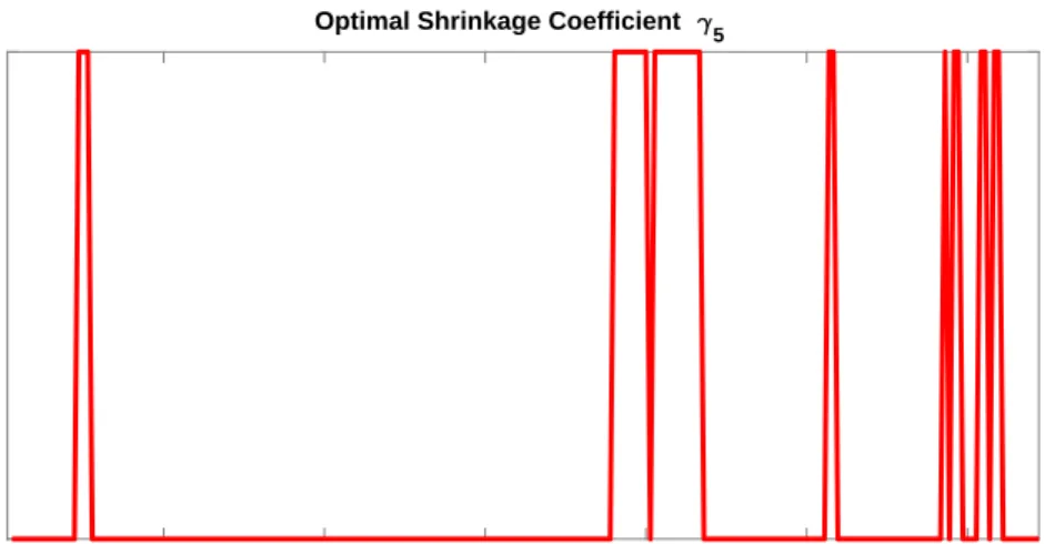
The Minnesota prior is typically controlled by a single shrinkage parameter, see Ba´nbura, Giannone, and Reichlin (2010) and citations therein. In order to deal with prior sensitivity associated with making a specification selection of this shrinkage parameter, Giannone, Lenza, and Primiceri (2015) and Koop and Korobilis (2013) use information in the data to learn about its value. We adopt a similar approach and allow the degree of shrinkage in the Minnesota prior to adaptively change over time. However, we go one step further by extending this prior to allow for richer shrinkage patterns. Instead of having one shrinkage parameter for all VAR coefficients, we allow for 10 independent shrinkage parameters (γ1, ..., γ10) that control the shrinkage of different sets of coefficients in our TVP-VAR models. In particular, we have a shrinkage parameter for intercepts,
12Discount factors are well established in finance; see the J.P. Morgan/Reuters (1996) Riskmetrics
model, and Dangl and Halling (2012) for a recent application in stock return predictability.
13Whenδ = 1 (similarly for λ), then the investor uses all available historical observations, equally
weighted, to update volatilities and parameters. For values less than one, older observations are
own lags, other lags and each individual asset-specific and non asset-specific variable. We choose a value for each of them from a grid of values which includes zero. Note that setting γi = 0 implies that the ith explanatory variable (or block of explanatory
variables) is excluded from the model. Hence, our method allows for the exclusion of predictors, if this is empirically warranted.
Full details of our statistical methods are given in the Technical Appendix.
3.2
Dynamic model learning
Estimation of a particular TVP-VAR-X involves setting each of δ, λ, γ1, ..., γ10 to a particular value. In practice, we consider a grid of values for all of these (see the Technical Appendix). If we consider every possible combination of values taken from all of these grids we have 9,216 choices of discount and shrinkage parameters. This is the number of models the investor has at their disposal at each point of time upon which they could base their portfolio allocation for the next period. In order to allow for the investor to make an optimal choice each period t, we introduce the notion of dynamic model learning. Dynamic model learning involves selecting, at each point in time, the model specification with the highest discounted joint log predictive likelihood up to that time. Predictive likelihood is a measure of out-of-sample forecasting ability that takes into account the shape of the forecast distribution and its higher moments (variance, skewness, etc.); see Geweke and Amisano (2012). The individual model configuration with the highest discounted joint log predictive likelihood is used in order to obtain the predictive mean and covariance matrix. These are a crucial input in portfolio optimization. Our motivation for using learning based on past forecast performance is that it allows for abrupt model changes. If we were to use a single TVP-VAR model, gradual parameter changes are accommodated if the discount factors δ and λ are below one. But this is not the same as switching between entirely different models as dynamic model learning allows for.
In this dynamic model learning setting, discounted joint predictive likelihood (DP L) can be calculated as DP Lt|t−1,j = t−1 Y i=1 pj yt−i|yt−i−1 αi ,
wherepj(yt−i|yt−i−1) denotes the predictive likelihood of modelj in periodiand t|t−1
time t−1. Hence, model j will receive a higher value at a given point in time if it has forecast well in the recent past, using the predictive likelihood (i.e., the predictive density evaluated at the actual outcome) as the evaluation criterion. The interpretation of “recent past” is controlled by the the discount factor α, modelling exponential decay. For example, if α = 0.95, forecast performance three years ago receives approximately 15% as much weight as the forecast performance last period. If α= 0.90, then forecast performance three years ago receives only about 2% as much weight. The case α = 1 implies no discounting and the discounted predictive likelihood is then proportional to the marginal likelihood. Lower values of α are associated with more rapid switching between models. We consider a range of values for αand, at each point in time, choose the best value for it. In this way, we can allow for times of fast model switching and times of slow model switching.
At time τ, we choose the best value for α as the one which has produced the model with the highest product of predictive likelihoods14 in the past from t = 1, ..., τ. We consider the following grid of values: α∈ {0.20; 0.40; 0.60; 0.80; 0.90; 0.95; 0.99; 1}. In the presence of instabilities, the choice of the estimation window is important for forecasting performance. Our real-time data-adaptive procedure to determine the empirically warranted degree of downweighting older data (controlled by λ for individual models and governed by α at the stage of model selection) addresses the need for choosing the appropriate window size for building forecasts and selecting models at each point in time.15
14We stress that we are not using theDP Lwhen choosing between different values forα. TheDP L
is only used to select the best model for a given value ofα.
15Pesaran and Pick (2011) provide evidence for both simulated and real data that combining forecasts
generated from the same model but over different estimation windows improves root mean squared errors compared to forecasts based on a single estimation window in the presence of a variety of instabilities. Similarly and more closely related to our work, Anderson and Cheng (2016) find that Bayesian model averaging of forecast models over different estimation windows leads to successful portfolio choice strategies, providing substantial out-of-sample utility gains for many common datasets. While Pesaran and Pick (2011) and Anderson and Cheng (2016) focus on combination of models which only differ by the estimation window but are otherwise identical, our setup considers both selecting among estimation windows for otherwise identical models (that is, models that are identical except for
λ) and also selecting estimation windows for models which are specified differently (for example with
respect to included regressors). Although implementation details differ, our strategy for choosing the empirically warranted degree of downweighting older data in presence of possible instabilities, is close in spirit to Pesaran and Pick (2011) and Anderson and Cheng (2016).
4
Dynamic asset allocation
4.1
Portfolio allocation
We design an international asset allocation strategy that involves trading the US dollar and seven other currencies. Consider a US investor who builds a portfolio by allocating their wealth between eight bonds: one domestic (US), and the seven foreign bonds. The US bond return is rf. Define yt= (y1,t, ..., y7,t)
0
. At each period, the foreign bonds yield a riskless return in the local currency but a risky return due to currency fluctuations in US dollars. The expectation of the risky return from the investment in countryi0sbonds, ri,t, at time t−1 is equal to Et−1(ri,t) =inti,t−1+yi,t.16 The only risk the US investor
is exposed to is foreign exchange (FX) risk. Every period the investor takes two steps. First, they use the currently selected model (i.e., the model with the highest discounted sum of predictive likelihoods) to forecast the one-period ahead exchange rate returns and the predictive covariance matrix. Second, using these predictions, they dynamically rebalance their portfolio by calculating the new optimal weights. This setup is designed to assess the economic value of exchange rate predictability and to dissect which sources of information are valuable for asset allocation.
We evaluate our models within a dynamic mean-variance framework, implementing a maximum expected return strategy. That is, we consider an investor who tries to find the point on the efficient frontier with the highest possible (ex-ante) return, subject to achieving a target conditional volatility and a given horizon of the investor (one-month ahead for our main results). Define rt = (r1,t, ..., r7,t)
0
, µt|t−1 = Et−1(rt)
as its expectation. The portfolio allocation problem involves choosing weights, wt= (w1,t, ..., w7,t)
0
attached to each of the 7 foreign bonds (with 1−P7
i=1wi,t being the weight attached to the domestic bond):
max wt µp,t|t−1 =w 0 tµt|t−1+ (1−w0tι)rf −τ ι0 wt−wt−1◦ 1 +rt 1 +rp,t subject to σ∗p2 = w0t δnt−1 δnt−1−2 xt−1Ωt|t−1x 0 t−1+Qt|t−1 | {z }
estimate of the predictive covariance matrix wt,
16We use y
i,t, the discrete exchange rate returns, rather than log returns ∆st, as, in the context of
where µp,t|t−1is the conditional expected portfolio return and σ∗p 2
the target portfolio variance. ι is a vector of ones and the arguments of the predictive covariance matrix are all produced by our estimation algorithm (see the Technical Appendix for definitions). We also here and below use notation where the portfolio return before transaction costs is Rp,t = 1 +rp,t−1 = 1 + 1−wt−0 1ι rf +w 0 t−1rt.
In addition, we let RT Cp,t denote period-t gross return after transaction costs, τ. Note that our specification of the portfolio allocation problem takes into account proportional transaction costs, τ, ex ante (i.e., at the time of the portfolio construction). Following Della Corte and Tsiakas (2012), we set τ = 0.0008. For our main results, we choose σp∗ = 10% as target portfolio volatility of the conditional portfolio returns.
4.2
Evaluation of economic utility
4.2.1 Quadratic utility
Mean-variance analysis is a natural framework for assessing the economic value of strategies that exploit predictability in the mean and covariance of a vector of risky assets. We use the West, Edison, and Cho (1993) methodology, which is based on mean-variance analysis with quadratic utility. The investor’s realized utility in period t can be written as U(Wt) = Wt− ρ 2W 2 t =Wt−1Rp,t− ρW2 t−1 2 (Rp,t) 2 , where Wt is the investor’s wealth in t, ρ determines their risk preferences.
We quantify the economic value of exchange rate predictability by setting the investor’s degree of relative risk aversion to θt = 1−ρWρWtt equal to a constant value θ.
We choose θ = 2 for our main results (and θ = 6 for robustness checks). In this case, West, Edison, and Cho (1993) demonstrate that one can use the average realized utility, U(·), to consistently estimate the expected utility generated by a given level of initial wealth. Specifically, the average utility for an investor with initial wealthW0 is equal to
U(·) =W0 (T−1 X t=0 Rp,tT C+1− θ 2 (1 +θ) R T C p,t+1 2 ) . (4)
risk aversion is constant and utility is homogenous in wealth. In contrast, for standard quadratic utility without restrictions on θ, relative risk aversion would be increasing in wealth, which is counterintuitive. Here, having constant relative risk aversion, we can setW0 = $1.
4.2.2 Performance measures
At any point in time, one set of estimates of the conditional mean and variance is better than a second set if investment decisions based on the first set lead to higher average realized utilityU. Alternatively, the optimal model requires less wealth to yield a given level of U than a suboptimal model. We measure the economic value of different forecasting approaches by equating the average utilities for selected pairs of portfolios. Suppose, for example, that holding a portfolio constructed using the optimal weights based on the random walk model yields the same average utility as holding the optimal portfolio based on a VAR model, which is subject to monthly expenses, expressed as a fraction Φ of wealth invested in the portfolio. Since the investor would be indifferent between these two strategies, we interpret Φ as the maximum performance fee they would be willing to pay to switch from the random walk to the specific VAR model. Hence, this utility-based criterion measures how much a mean-variance investor is willing to pay for conditioning on a particular VAR configuration. The performance fee will depend on the investor’s degree of risk aversion. To estimate the fee, we find the value of Φ that satisfies T−1 X t=0 Rp,tT C,∗+1−ΦT C − θ 2 (1 +θ) RT C,∗p,t+1−ΦT C 2 = T−1 X t=0 RT Cp,t+1− θ 2 (1 +θ) R T C p,t+1 2 , (5) where RT C,∗p,t+1 is the gross portfolio return constructed using using the expected return and covariance forecasts from the dynamically selected best model configuration and Rp,tT C+1 is implied by the benchmark random walk (without drift) model. The superscript
TC indicates that all quantities are computed after adjusting for transaction costs. In the context of mean-variance analysis, a commonly used measure of economic value is the Sharpe ratio. However, as suggested by Marquering and Verbeek (2004) and Han (2006), the Sharpe ratio can be misleading because it severely underestimates the performance of dynamic strategies. Specifically, the realized Sharpe ratio is computed using the sample standard deviation of the realized portfolio returns. Hence it
overestimates the conditional risk an investor faces at each point in time. Furthermore, the Sharpe ratio cannot quantify the exact economic gains of dynamic strategies over a static random walk strategy in the same direct and easy to interpret way of the performance fee. Therefore, our economic analysis of short-horizon exchange rate predictability focuses primarily on performance fees, while Sharpe ratios of selected models are reported as a second measure of economic performance. In our empirical analysis, we report annualized Sharpe ratios and adjust for the serial correlation in the monthly portfolio returns generated by the dynamic strategies.17
5
Empirical results
5.1
Evidence on model switching
Our most flexible specification allows for dynamic model learning over a set of 9,216 different TVP-VAR-X models and eight different values ofαusing the methods described in Section 3. We will refer to this as the DML-TVP-VAR-X in the table and discussion below. We also consider a range of special cases of this unrestricted specification. Our focus is on how well these specifications perform in terms of our dynamic asset allocation problem. However, before doing this, we present a few results illustrating how the dynamic model learning strategy is working in the most flexible specification.
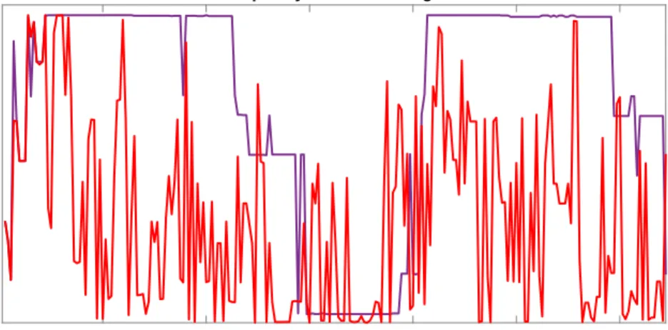
Dynamic model learning is to be preferred over static Bayesian model learning only if the optimal forecasting model is changing over time. Figure 1 shows that it does so in our application. The vertical axis plots the model numbers from 1 to 9,216 against time for two cases. The first uses our DML-TVP-VAR-X specification (which allows for α be be selected in a time-varying manner)18 and the second sets α = 1. Both cases show that different models are selected at different times. But with our flexible specification whereαis chosen in real time, the model change is dramatic. It is choosing a wide range of different models. Figure 1 establishes that model change is occurring, but does not directly inform the reader as to which models are selected. Remember that these models differ in which lagged endogenous and exogenous variables are included and the degree
17Following Lo (2002), we multiply monthly Sharpe ratios by the adjustment factor 12
s 12+2 11 P k=1 (12−k)ρk ,
whereρk is the autocorrelation coefficient of portfolio returns at lag k.
18As we includeα= 1 as a grid point in the flexible version, static model learning is included in this
1999:09 2002:09 2005:09 2008:09 2011:09 2014:09 Frequency of Model Change
Figure 1: The figure displays the frequency of model change over time. The vertical axis represents the model configurations 1, ...,9,216. The purple line depicts the evolution of the selected model configuration for α = 1. The red line shows the evolution of the selected model configuration for α∈ {0.2,0.4; 0.6; 0.8; 0.9; 0.95; 0.99; 1}.
of time variation in the model parameters. Figure 2 relates to the seven exogenous variables and plots the number of them chosen at each point in time by DML-TVP-VAR-X. There is only one period (and that is at the time of the financial crisis) where all seven of the exogenous variables are included. Instead the story is one of change. Most of the time only a few of the exogenous predictors are chosen (the average over time of all the numbers in Figure 2 is 2.05) and there are several periods where none of them are chosen. Thus, the optimal small set of fundamentals quickly changes over time which aligns with the theory (Bacchetta and van Wincoop, 2004; Markiewicz, 2012). Altogether, our method appears to capture the unstable link between fundamentals and exchange rates.
5.2
Out-of-sample forecast evaluation
The previous sub-section established that our DML-TVP-VAR-X approach was picking up model change. But the key issue is whether this is important for forecast performance. In this sub-section we report various performance measures based on two economic criteria and one statistical criterion: the performance fee after transaction costs (ΦT C), the Sharpe ratio before and after transactions costs (SR and SRT C) as well as the joint predictive log likelihood (P LL). The last measures the accuracy of the density forecasts.
1999:09 2002:09 2005:09 2008:09 2011:09 2014:09 0 1 2 3 4 5 6
7 Number of Included Regressors
Figure 2: The figure displays the number of included regressor at each point in time. Included means that the associated hyperparameter γ 6= 0 is selected.
The two economic criteria are benchmarked relative to a random walk without drift and constant volatility. Hence, the performance fee ΦT C is the annualized fee a risk-averse investor (with risk aversion θ = 2) is willing to pay for switching from a dynamic portfolio strategy based on the random walk model to one that conditions on a more flexible forecasting strategy.
In addition to the DML-TVP-VAR-X, we compare our results to a range of restricted versions thereof so as to investigate which aspects of our approach are most important. That is, we can disentangle whether exclusion of certain sets of variables or individual variables, time variation of the coefficients or the covariance matrix or the dynamics of the model selection procedure are the most important features in ensuring good performance according to our performance measures. Table 1 contains our results.
The DML-TVP-VAR-X can be seen to perform very well in terms of our economic performance indicators. The annualized performance fee after transaction costs is 739 basis points (bps) and the annualized Sharpe ratio is 1.33 before transaction costs and 1.16 after transaction costs. The figures are the highest or nearly highest of any in Table 1 and are substantially better than most alternatives. When looking at the statistical performance, the joint predictive log likelihoods also show that DML-TVP-VAR-X is among the best, although here the differences between models are not as large as they are with the economic performance measures. The joint predictive likelihood and the
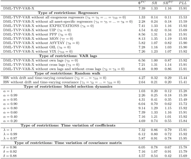
Table 1: Evaluation of forecasting results.
The table summarizes the economic and statistical evaluation of our forecasts of the DML-TVP-VAR-X model and restricted versions thereof for the period from 2004:01 to 2015:12. As our main economic
evaluation criterion, we report the annualized fee which a risk-averse investor withθ= 2 andσ∗p= 10%
is willing to pay to switch from the naive random walk strategy to a more flexible forecasting strategy.
This annualized fee is reported after taking into account transaction costs as ΦT C. We consider
proportional transaction costs of 8 basis points. As a second measure of economic utility, we report
the annualized Sharpe ratio before transaction costs (SR) and after transaction costs (SRT C). As
a statistical measure for the accuracy of the density forecasts, we report the joint predictive log likelihoods (PLL).
ΦT C SR SRT C P LL
DML-TVP-VAR-X 7.39 1.33 1.16 15.91
Type of restrictions: Regressors
DML-TVP-VAR without all exogenous regressors (γ4=γ5=...=γ10= 0) 1.33 0.14 0.11 15.53
DML-TVP-VAR-X without all asset-specific regressors (γ4=γ5=...=γ8= 0) 2.28 0.24 0.18 15.59
DML-TVP-VAR-X without EXPECTATIONS (γ4= 0) 7.41 1.33 1.16 15.92
DML-TVP-VAR-X without UIP (γ5= 0) 4.54 0.42 0.34 15.69
DML-TVP-VAR-X without PPP (γ6= 0) 8.56 1.31 1.16 15.91
DML-TVP-VAR-X without MON (γ7= 0) 8.13 1.35 1.19 15.93
DML-TVP-VAR-X without ASYTAY (γ8= 0) 5.82 1.07 0.82 15.90
DML-TVP-VAR-X without OIL (γ9= 0) 7.28 1.16 1.03 15.90
DML-TVP-VAR-X without VIX (γ10= 0) 7.26 1.23 1.07 15.92
Type of restrictions: VAR lags
DML-TVP-VAR-X without own lags (γ2= 0) 6.56 1.00 0.87 15.92
DML-TVP-VAR-X without cross lags (γ3= 0) 7.21 1.31 1.14 15.91
DML-TVP-VAR-X without own lags and without cross lags (γ2=γ3= 0) 6.48 0.99 0.86 15.91
Type of restrictions: Random walk
RW with drift and time-varying covariance (γ2=...=γ10= 0) 4.27 0.32 0.29 15.44
RW without drift and time-varying covariance (γ1=γ2=...=γ10= 0) 2.64 0.21 0.20 15.41
Type of restrictions: Model selection dynamics
α= 1 1.03 0.20 0.12 15.28 α= 0.99 2.26 0.25 0.18 15.39 α= 0.95 4.31 0.41 0.35 15.49 α= 0.90 6.04 0.70 0.62 15.72 α= 0.80 9.14 1.29 1.15 15.92 α= 0.60 7.39 1.33 1.16 15.91 α= 0.40 7.16 1.21 1.01 15.92 α= 0.20 4.69 0.74 0.55 15.84
Type of restrictions: Time variation of coefficients
λ= 1 7.32 0.86 0.79 15.91
λ= 0.99 6.12 0.80 0.72 15.92
λ= 0.97 5.87 0.91 0.78 15.95
Type of restrictions: Time variation of covariance matrix
δ= 0.96 6.05 0.78 0.67 15.78
δ= 0.92 7.16 1.07 0.91 15.79
δ= 0.88 4.57 0.54 0.42 15.69
two economic criteria broadly agree with respect to the ranking of the models.19
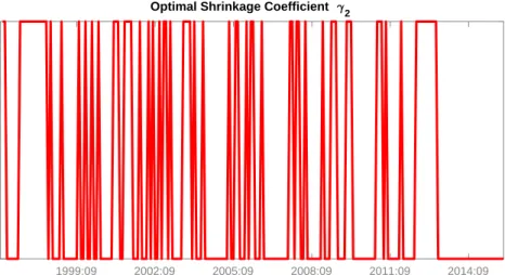
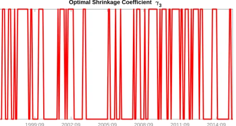
We now turn to an investigation of what aspects of DML-TVP-VAR-X are most important in leading to its good performance beginning with a discussion of the hyperparameters, γ, which relate to the inclusion or exclusion of explanatory variables. Figures 4 to 12 in our Empirical Appendix show exactly which of these are included or excluded at each point in time. A general pattern in these figures is that there is a lot of dynamic switching relating to which of the variables enter or leave the model. Table 1 shows what happens when we impose restrictions that various coefficients are omitted from the model at all points in time. For most cases, completely excluding an explanatory variable leads to large drops in all of our performance measures. Excluding economic fundamentals altogether leads to a substantial deterioration in the portfolio performance. This also holds true for the case where only asset-specific exogenous variables are excluded. If we exclude the asset-specific exogenous variables, the annualized fee drops from 7.39% to 2.28%, while the Sharpe ratio falls from 1.16 to 0.18 after transaction costs. Additionally excluding the non asset-specific predictors (OIL, VIX) leads to even worse results (ΦT C = 1.33, SRT C = 0.11). Similarly, DML-TVP-VAR-X outperforms
the random walk specifications. Note that if we add a time-varying covariance matrix to the random walk configurations it leads to improved performance over the homoskedastic random walk with constant covariance matrix. However, these improvements are much less than we found with DML-TVP-VAR-X. Overall, this is clear-cut evidence that including exogenous variables improves the economic performance and that our setup is in fact able to capture the unstable link between fundamentals and exchange rates.
With regards to the individual exogenous variables, UIP in particular appears to contain useful information since performance fees and the Sharpe ratio both drop substantially in a configuration that excludes this variable. Inspection of Figure 7 in the Empirical Appendix reveals that UIP has been included particularly during the subprime crisis. However, the exclusion of PPP does not lead to any such deterioration. Given the existing evidence on slow mean reversion in real exchange rates and the low inflation environment throughout our evaluation period, the finding that PPP is not generating economic utility is not surprising. We also find appreciable losses from excluding the asymmetric Taylor rule (ASYTAY), although these are smaller than those which occur if UIP is excluded. This might be explained by the emergence of the
zero-They report broad agreement between density forecast measures and economic performance measures. Instead, there is typically a weak link between point forecast evaluation criteria and economic evaluation criteria.
lower bound and unconventional monetary policy which implies that interest rate setting is not characterized by standard Taylor rules over the full sample. We do not find any economic or statistical improvement from considering monetary fundamentals nor from considering survey data. This pattern aligns with the finding that the predictive power of exchange rate expectations often turns out to be rather weak.
Another interesting finding is that excluding both non asset-specific variables (OIL and VIX) decreases performance substantially, but excluding them individually only marginally reduces the various performance measures. Finally, excluding own and/or cross VAR lags leads to only a small reduction in our economic utility measures.
We next delineate the effects of restrictions on the tuning parameters α, δ and λ. Previously, in Figure 1, we showed that the optimal model can rapidly change over time. The results in Table 1 relating to α show the benefits of this for forecasting. Fixing α = 1 rather than choosing the value of α in real time leads to very poor forecasting results (ΦT C = 1.03, SRT C = 0.12). Allowing for lower values ofαand, thus, more model
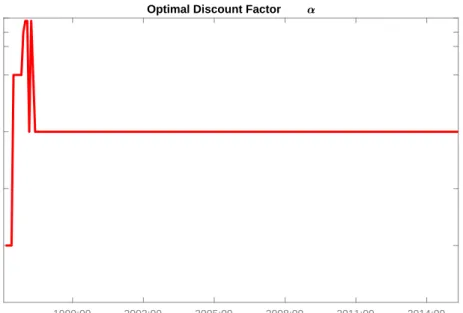
switching leads to higher values of the performance fee and the Sharpe ratio. In fact, the highest performance fee is obtained when α = 0.80 and the highest Sharpe ratios when α = 0.60. Thus, large economic and statistical losses occur if the investor does not emphasize the most recent forecast performance when selecting the forecast model on which to base their asset allocation decision. Figure 3 plots the value of α selected by our DML-TVP-VAR-X approach at each point in time. It shows that α = 0.60 is chosen in real time during the entire evaluation period which begins in 2004. Hence, the results for the model configuration with the restriction α = 0.60 and the results for the DML-TVP-VAR-X, are identical. Altogether, the choice of the discount factor α for controlling the degree of likelihood discounting is a very important one here so as to handle frequent changes of relevant fundamentals.
In terms of time variation in parameters, imposing λ = 1 and, thus, constant coefficients on lagged dependent and exogenous variables has little effect, although the Sharpe ratio is somewhat reduced.20 Fixing λ = 0.99 or 0.97 and, thus, imposing gradual parameter change does lead to some reduction in performance fees, although our measure of statistical performance is increased by doing so. With DML-TVP-VAR-X, different degrees of time variation are selected over time (see Figure 14 in the Empirical
20 This discrepancy between the performance fee and the Sharpe ratio may stem from the fact that
we account for autocorrelation in monthly returns when calculating the Sharpe ratio, while we do not so when calculating the performance fee.
1999:09 2002:09 2005:09 2008:09 2011:09 2014:09 0.2 0.4 0.6 0.8 0.9 0.95
1 Optimal Discount Factor
Figure 3: The figure diplays the selected values of the discount factor α ∈
{0.2; 0.4; 0.6; 0.8; 0.9; 0.95; 0.99; 1} over time.
Appendix). It is interesting to note that, while economic and statistical criteria are in line for most of the model configurations, they are not for the restrictions on λ.
All our model configurations are heteroskedastic.21 However, the degree of time variation of the covariance matrix is controlled by different possible values of the discount factor δ. Fixing δ comes with losses in economic and statistical measures, providing evidence that the degree of volatility varies through time (see Figure 13 in the Empirical Appendix). The degree of volatility will directly effect the variance of the predictive density which, in turn, will affect predictive credible intervals. Figure 17 in our Empirical Appendix plots 90% credible intervals along with the actual realizations for our 7 exchange rates. The credibility intervals are quite precisely estimated and have good coverage (approximately 9% of actual observations are outside the 90% credibility intervals if we average over exchange rates and time). This provides evidence that our dynamic selection of δ is successful in capturing the volatility in the data.
21Including homoskedastic models with a constant covariance matrix is easily accomplished in our
setting by including an additional grid pointδ= 1. However, when includingδ= 1, this grid point is
6
Robustness checks and extensions
6.1
Subsample analysis
To shed some light on the robustness of our findings, Table 2 presents the same results as Table 1, but for three sub-periods: 2004:01 − 2007:12, 2008:01− 2011:12 and 2012:01−2015:12. For brevity, we only present results for DML-TVP-VAR-X and a sub-set of our models. We find that DML-TVP-VAR-X provides large economic gains throughout all three subperiods. This robustness is corroborated by Figures 15 and 16 in the Empirical Appendix which depict the evolution of the performance fee and wealth over time. Excluding all regressors as a block (TVP-VAR) or adopting a random walk specification with time-varying covariance leads to very poor forecasting results during the second subperiod which contains the subprime crisis. This points to the importance of including exogenous regressors during turbulent market times and aligns with the implication of Figure 2.
Excluding the professional forecasts (EXPECTATIONS) does not affect the results in any subperiod. UIP turns out to be an important predictor in the second sub-period which corresponds to the times in which UIP is included in the model (see Figure 7). The importance of UIP in the second subperiod is potentially related to the collapse of carry trades due to the narrowing of interest rate differentials after 2008. Changes in small interest rate differentials seem to incorporate information about future exchange rate movements between 2008 and 2011. PPP and MON do not provide any economic utility for any subsample. ASYTAY turns out to be quite important in the first subperiod, reflecting the fact that Taylor rules provide an arguably reasonable characterization of monetary policy prior to the low-interest rate environment. Fast model switching accomplished by low values ofαwas particularly important between 2008:01 and 2011:12, the period containing the subprime crisis. However, fixing α = 1 would have been a poor choice in any subperiod, while adopting constant coefficients (λ = 1) was only detrimental in the second subperiod.
T able 2: Ev aluation of sub-p erio d results. The table summarizes the e conomic and statistical ev aluati on of our forecasts for thr e e sub-sample p erio ds: 2004:01 − 2007:12, 2008:01 − 2011:12 and 2012:01 − 2015:12. W e rep ort the ann ualized fee whic h a risk-a v erse in v estor with θ = 2 and target p ortfolio v olatilit y σ ∗ p = 10% is willing to pa y to switc h from the naiv e random w alk strategy to a more flexible forecasting strategy . This ann ualized fee is rep orted after taking in to accoun t transaction c osts as Φ T C. W e consider prop ortional transac ti on costs of 8 basis p oin ts. W e also rep or t the ann ualized Sharp e ratio after tran saction costs ( S R T C ). Φ T C S R T C 04 : 07 08 : 11 12 : 15 04 : 07 08 : 11 12 : 15 DML-TVP-V AR-X 5 . 94 8 . 82 7 . 39 1 . 46 1 . 26 0 . 78 T yp e of restrictions: Regressors DML-TVP-V AR without all exogenous regressors ( γ4 = γ5 = ... = γ10 = 0) 7 . 29 − 9 . 63 6 . 47 1 . 32 − 0 . 29 0 . 45 DML-TVP-V AR-X without all asset-sp ecific regressors ( γ4 = γ5 = ... = γ8 = 0) 4 . 22 − 4 . 78 7 . 44 1 . 15 − 0 . 18 0 . 58 DML-TVP-V AR-X without EXPE CT A TIONS ( γ4 = 0) 5 . 94 8 . 82 7 . 39 1 . 46 1 . 26 0 . 78 DML-TVP-V AR-X without UIP ( γ5 = 0) 5 . 94 − 2 . 93 10 . 67 1 . 46 − 0 . 15 1 . 00 DML-TVP-V AR-X without PPP ( γ6 = 0) 6 . 56 9 . 49 9 . 61 1 . 16 1 . 47 1 . 26 DML-TVP-V AR-X without MON ( γ7 = 0) 6 . 26 9 . 07 9 . 04 1 . 59 1 . 21 0 . 86 DML-TVP-V AR-X without ASYT A Y ( γ8 = 0) 3 . 16 8 . 19 6 . 10 0 . 86 1 . 20 0 . 50 T yp e of restrictions: Random w alk R W without drift and time-v arying co v ariance ( γ1 = γ2 = ... = γ10 = 0) 8 . 82 − 3 . 68 3 . 05 1 . 47 − 0 . 14 0 . 08 T yp e of restrictions: Mo del selection dynamics α = 1 4 . 31 − 3 . 36 2 . 16 1 . 24 − 0 . 23 − 0 . 05 α = 0 . 99 4 . 12 − 5 . 79 8 . 48 1 . 14 − 0 . 35 0 . 45 α = 0 . 95 6 . 91 − 2 . 25 8 . 34 1 . 51 − 0 . 09 0 . 51 α = 0 . 90 5 . 10 3 . 36 9 . 64 1 . 34 0 . 26 0 . 70 α = 0 . 80 6 . 23 10 . 29 10 . 85 1 . 34 1 . 18 0 . 99 α = 0 . 60 5 . 94 8 . 82 7 . 39 1 . 46 1 . 26 0 . 78 α = 0 . 40 5 . 89 6 . 37 9 . 21 1 . 54 0 . 70 1 . 00 α = 0 . 20 6 . 05 2 . 80 5 . 23 1 . 58 0 . 20 0 . 37 T yp e of restrictions: Time v ariation of co efficien ts λ = 1 4 . 93 5 . 62 11 . 37 1 . 09 0 . 52 0 . 95
6.2
Currency selection
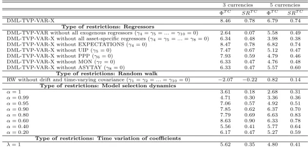
Another important robustness check corresponds to the choice of currencies. We re-estimate our models for two alternative country settings. The first considers three currencies vis-`a-vis the US dollar: GBP, Euro and JPY. The second considers five currencies vis-`a-vis the US dollar: GBP, Euro, JPY, Canadian dollar and Australian dollar. We report the performance fees and Sharpe ratios after transaction costs, respectively. Table 3 summarizes the results. With respect to excluding exogenous regressors as a block and the restrictions on α and λ we observe similar patterns as for our main results. However, we do observe some different patterns with respect to the importance of certain regressors compared to the main setting. While excluding PPP and MON even improves the findings for our main setting, the performance weakens for both alternative currency selections.
6.3
Choice of risk aversion and target volatility
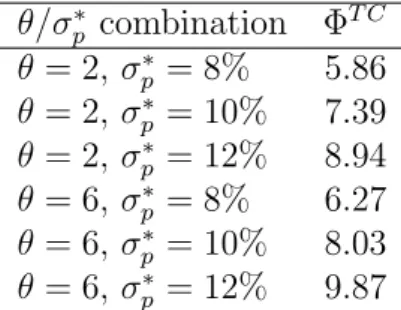
Having assessed the robustness in terms of sample and country choice, we modify our assumptions related to the utility function of the investor. Table 4 provides estimates of the annualized performance fee after transaction costs using our DML-TVP-VAR-X approach for two different degrees of risk aversion (θ ∈ {2,6}) and three different values of the target portfolio volatility σ∗p ∈ {8%,10%,12%}
. It is worth reiterating that our main results were reported for θ = 2 and σp∗ = 10%. The results document that the performance fee increases with higher target portfolio volatilities and is higher for θ=6 compared to θ = 2, keeping σp∗ constant. These findings document that the reported base case results are unlikely to overstate the utility gains of a representative investor.
6.4
Choice of benchmark
Our previous findings use the random walk without drift (and a constant covariance
matrix) as a benchmark. This provides arguably the toughest comparison when
evaluating exchange rate forecasts (Rossi, 2013). Moving to the random walk with drift (and a constant covariance matrix) as a benchmark leads to even more striking performance of DML-TVP-VAR-X with ΦT C = 12.93 when we setθ = 2 and σ∗p = 10% as above.
Table 3: Evaluation of results for alternative currency selections.
The table summarizes the economic evaluation of our forecasts for two alternative currency selections
including three and five currencies vis`a-vis the US dollar. The three-country setting comprises GBP,
EUR and the JPY while the five-country setting comprises GBP, EUR, JPY, CAD and AUD. We
report the annualized fee which a risk-averse investor with θ = 2 and target portfolio volatility
σ∗p = 10% is willing willing to pay to switch from the naive random walk strategy to a more flexible
forecasting strategy. This annualized fee is reported after taking into account transaction costs as ΦT C.
We consider proportional transaction costs of 8 basis points. We also report the annualized Sharpe
ratio after transaction costs (SRT C).
3 currencies 5 currencies ΦT C SRT C ΦT C SRT C
DML-TVP-VAR-X 8.46 0.78 6.79 0.74
Type of restrictions: Regressors
DML-TVP-VAR without all exogenous regressors (γ4=γ5=...=γ10= 0) 2.64 0.07 5.58 0.49 DML-TVP-VAR-X without all asset-specific regressors (γ4=γ5=...=γ8= 0) 6.34 0.48 3.98 0.38 DML-TVP-VAR-X without EXPECTATIONS (γ4= 0) 8.47 0.78 6.82 0.74 DML-TVP-VAR-X without UIP (γ5= 0) 7.47 0.67 5.12 0.47 DML-TVP-VAR-X without PPP (γ6= 0) 7.93 0.59 4.79 0.46 DML-TVP-VAR-X without MON (γ7= 0) 6.33 0.47 4.76 0.48 DML-TVP-VAR-X without ASYTAY (γ8= 0) 6.33 0.47 5.57 0.60
Type of restrictions: Random walk
RW without drift and time-varying covariance (γ1=γ2=...=γ10= 0) −2.07 −0.22 0.82 0.14
Type of restrictions: Model selection dynamics
α= 1 3.61 0.18 2.68 0.31 α= 0.99 4.71 0.30 3.36 0.36 α= 0.95 7.06 0.57 4.92 0.51 α= 0.90 7.85 0.62 6.37 0.70 α= 0.80 7.79 0.69 6.63 0.83 α= 0.60 8.63 0.90 6.33 0.78 α= 0.40 5.56 0.41 5.77 0.64 α= 0.20 6.17 0.47 5.27 0.59
Type of restrictions: Time variation of coefficients
λ= 1 5.62 0.35 4.80 0.41
6.5
Further robustness checks and extensions
We have performed several additional robustness tests which are left out for brevity but are available upon request. These do not change our main findings. The additional robustness checks include the use of three-month ahead forecasts, risk-adjustment of interest rates via forward rates, Euribor instead of LIBOR interest rates, alternative grid values for the Minnesota shrinkage priors, and a symmetric Taylor rule instead of an asymmetric one. As an alternative performance measure we also investigated the manipulation-proof performance measure proposed by Goetzmann, Ingersoll, Spiegel, and Welch (2007). The advantage of this criterion is that we neither have to assume a particular return distribution nor a certain utility function. The results compared to the reported quadratic utility case are very similar.
Table 4: Risk aversion and target portfolio volatility.
The table reports the economic value of of the DML-TVP-VAR-X model for several combinations of
risk aversionδand target volatilityσ∗p = 10. This annualized fee is reported after taking into account
transaction costs as ΦT C. We consider proportional transaction costs of 8 basis points.
θ/σp∗ combination ΦT C θ = 2, σ∗p = 8% 5.86 θ = 2, σ∗p = 10% 7.39 θ = 2, σ∗p = 12% 8.94 θ = 6, σ∗p = 8% 6.27 θ = 6, σ∗p = 10% 8.03 θ = 6, σ∗p = 12% 9.87
Note that the portfolio weights are not restricted in our base setting and vary widely over time (see Figure 18 in the Empirical Appendix). The average annual portfolio turnover implied by the VAR model is 11.73 compared to 1.37 (4.03) implied by the random walk model without (with) drift and stochastic volatility. We have considered restrictions on minimum and maximum portfolio weights and maximum portfolio turnover. We did not find any gains in terms of portfolio performance in incorporating such restrictions. To minimize transaction costs we also considered a strategy which involves trading a mixture of the current portfolio and the target portfolio weights. The fact that neither the mixture strategy nor restrictions on portfolio weights/turnover restrictions improve the overall results points to a scenario in which the gains due to reducing transaction costs are offset by partly ignoring the signals provided by the forecasting model.
We have exploited the flexibility of our method by including additional regressors. We have included either the highest and lowest forecast (standardized by the expected forecast) or the absolute difference between both values (standardized by the expected forecast) as a measure of disagreement among exchange rate forecasters. These do not change our results.
If we exclude Chile and South Korea, we can extend our sample back to 1975. Similar to Table 3, our main results again remain unaltered in the sense that we also identify substantial economic gains and find rapid model changes with typically only a small set of relevant fundamentals at each point in time.
As a further robustness check, we extended our framework to accommodate third-country effects of exchange rates recently highlighted by Berg and Mark (2015). That is, including exogenous variables specific to an asset in the equation for other assets. The results are not noticably affected by incorporating such spillover effects.
An interesting extension of our framework would involve combining the time-series signals provided by our proposed approach with some long-short style-based FX strategies such as carry, momentum or value reversal (see, for example, Barroso and Santa-Clara (2015)). Such style-based FX strategies exploit the cross section of the FX returns and may provide useful complementary information in addition to the time-series signals. Blending cross-section and times-time-series signals could lead to an even more robust performance and could help reduce transaction costs. The weights attached to the time-series and cross-section strategies could be determined by directly optimizing an investor’s utility in the framework of Brandt, Santa-Clara, and Valkanov (2009).
7
Concluding remarks
This paper has proposed a new multivariate forecasting approach for exchange rate returns. Our dynamic Bayesian learning approach enables us to quickly detect model changes over time and achieves computational feasibility by using decay factors. A major conceptual advantage of our approach over univariate models is that we obtain the input for the inherently multivariate portfolio otimization problem in a natural manner without having to rely on additional assumptions and procedures for mapping the forecast output into portfolio weights.
We have evaluated the economic value of our exchange rate forecasts in a dynamic asset allocation framework. Relying on our forecasting method, an investor achieves sizeable utility gains by capturing short-lived predictability. Our findings hold up to a large set of robustness tests. The time-varying importance of fundamentals and the frequent model shifts align with the implications of the theoretical and empirical exchange rate literature. Our forecasting strategy takes into account several dimensions of uncertainty. It is encouraging that the flexibility embedded in our approach pays off, particularly around the subprime crisis.
References
Abhyankar, A., L. Sarno, and G. Valente (2005): “Exchange rates and
fundamentals: evidence on the economic value of predictability,” Journal of
International Economics, 66(2), 325–348.
Anderson, E. W., and A.-R. Cheng (2016): “Robust bayesian portfolio choices,”
The Review of Financial Studies, 29(5), 1330–1375.
Bacchetta, P., and E. van Wincoop (2004): “A Scapegoat Model of
Exchange-Rate Fluctuations,” American Economic Review, 94(2), 114–118.
(2006): “Can Information Heterogeneity Explain the Exchange Rate
Determination Puzzle?,”American Economic Review, 96(3), 552–576.
(2013): “On the unstable relationship between exchange rates and
macroeconomic fundamentals,”Journal of International Economics, 91(1), 18–26.
Bakshi, G., and G. Panayotov (2013): “Predictability of currency carry trades and
asset pricing implications,”Journal of Financial Economics, 110(1), 139–163.
Ba´nbura, M., D. Giannone, and L. Reichlin(2010): “Large Bayesian vector auto
regressions,”Journal of Applied Econometrics, 25(1), 71–92.
Barroso, P., and P. Santa-Clara (2015): “Beyond the carry trade: Optimal
currency portfolios,” Journal of Financial and Quantitative Analysis, 50(5), 1037– 1056.
Beckmann, J., and R. Sch¨ussler (2016): “Forecasting exchange rates under
parameter and model uncertainty,”Journal of International Money and Finance, 60, 267–288.
Berg, K. A., and N. C. Mark (2015): “Third-country effects on the exchange rate,”
Journal of International Economics, 96(2), 227–243.
Bilson, J. F. O. (1978): “The Current Experience with Floating Exchange Rates: An
Appraisal of the Monetary Approach,”American Economic Review, 68(2), 392–397.
Blake, D., M. Beenstock, and V. Brasse (1986): “The performance of UK
Brandt, M. W., P. Santa-Clara, and R. Valkanov (2009): “Parametric
portfolio policies: Exploiting characteristics in the cross-section of equity returns,”
The Review of Financial Studies, 22(9), 3411–3447.
Byrne, J. P., D. Korobilis, and P. J. Ribeiro (2016): “Exchange rate
predictability in a changing world,” Journal of International Money and Finance, 62, 1–24.
Carriero, A., G. Kapetanios,andM. Marcellino(2009): “Forecasting exchange
rates with a large Bayesian VAR,” International Journal of Forecasting, 25(2), 400– 417.
Cavusoglu, N., and A. R. Neveu (2015): “The Predictive Power of Survey-Based
Exchange Rate Forecasts: Is there a Role for Dispersion?,” Journal of Forecasting, 34(5), 337–353.
Cenesizoglu, T., and A. Timmermann (2012): “Do return prediction models add
economic value?,”Journal of Banking & Finance, 36(11), 2974–2987.
Chib, S., F. Nardari, and N. Shephard (2006): “Analysis of high dimensional
multivariate stochastic volatility models,”Journal of Econometrics, 134(2), 341–371.
Chinn, M., and J. Frankel (1994): “Patterns in Exchange Rate Forecasts for
Twenty-Five Currencies,”Journal of Money, Credit and Banking, 26(4), 759–770.
Dangl, T., and M. Halling (2012): “Predictive regressions with time-varying
coefficients,”Journal of Financial Economics, 106(1), 157–181.
Della Corte, P., L. Sarno, and I. Tsiakas (2008): “An economic evaluation of
empirical exchange rate models,”The Review of Financial Studies, 22(9), 3491–3530.
Della Corte, P., and I. Tsiakas (2012): “Statistical and economic methods for
evaluating exchange rate predictability,” Handbook of exchange rates, pp. 221–263.
Dornbusch, R. (1976): “Expectations and Exchange Rate Dynamics,” Journal of
Political Economy, 84(6), 1161–1176.
Engel, C. (2013): “Exchange Rates and Interest Parity,” NBER Working Papers