Tests of Mean-Variance Spanning
Raymond Kan
Rotman School of Management, University of Toronto, Canada E-mail: [email protected]
and
GuoFu Zhou*
Olin Business School, Washington University, St. Louis, USA E-mail: [email protected]
In this paper, we conduct a comprehensive study of tests for mean-variance spanning. Under the regression framework of Huberman and Kandel (1987), we provide geometric interpretations not only for the popular likelihood ra-tio test, but also for two new spanning tests based on the Wald and Lagrange multiplier principles. Under normality assumption, we present the exact distri-butions of the three tests, analyze their power comprehensively. We find that the power is most driven by the difference of the global minimum-variance portfolios of the two minimum-variance frontiers, and it does not always align well with the economic significance. As an alternative, we provide a step-down test to allow better assessment of the power. Under general distributional as-sumptions, we provide a new spanning test based on the generalized method of moments (GMM), and evaluate its performance along with other GMM tests by simulation.
Key Words: Mean-variance spanning; Spanning tests; Portfolio efficiency. JEL Classification Numbers:G11,G12,C11.
* We thank an anonymous referee, Stephen Brown, Philip Dybvig, Wayne Ferson, Chris Geczy, Gonzalo Rubio Irigoyen, Bob Korkie, Alexandra MacKay, Shuzhong Shi, Tim Simin, seminar participants at Beijing University, Fields Institute, Indiana Univer-sity, University of California at Irvine, York UniverUniver-sity, and participants at the 2000 Northern Finance Meetings, the 2001 American Finance Association Meetings, and the Third Annual Financial Econometrics Conference at Waterloo for helpful discussions and comments. Kan gratefully acknowledges financial support from the National Bank Financial of Canada.
145
1529-7373/2012 All rights of reproduction in any form reserved.
1. INTRODUCTION
In portfolio analysis, one is often interested in finding out whether one set of risky assets can improve the investment opportunity set of another set of risky assets. If an investor chooses portfolios based on mean and variance, then the question becomes whether adding a new set of risky assets can allow the investor to improve the minimum-variance frontier from a given set of risky assets. This question was first addressed by Huberman and Kandel (1987, HK hereafter). They propose a multivariate
test of the hypothesis that the minimum-variance frontier of a set of K
benchmark assets is the same as the minimum-variance frontier of theK
benchmark assets plus a set of N additional test assets. Their study has
generated many applications and various extensions. Examples include Ferson, Foerster, and Keim (1993), DeSantis (1993), Bekaert and Urias (1996), De Roon, Nijman, and Werker (2001), Korkie and Turtle (2002), Ahn, Conrad, and Dittmar (2003), Jagannathan, Skoulakis, and Wang (2003), Pe˜naranda and Sentana (2004), Christiansen, Joensen, and Nielsen (2007), and Chen, Chung, Ho and Hsu (2010).
In this paper, we aim at providing a complete understanding of various tests of mean-variance spanning.1 First, we provide two new spanning tests based on the Wald and Lagrange multiplier principles. The popular HK spanning test is a likelihood ratio test. Unlike the case of testing the CAP-M as in Jobson and Korkie (1982) and Gibbons, Ross, and Shanken (1989, GRS hereafter), this test is in general not the uniformly most powerful invariant test (as shown below), and hence the new tests are of interest. Second, we provide geometrical interpretations of the three tests in terms of theex postminimum-variance frontier of theKbenchmark assets and that of the entireN+Kassets, which are useful for better economic understand-ing of the tests. Third, under the normality assumption, we present the small sample distributions for all of the three tests, and provide a complete analysis of their power under alternative hypotheses. We relate the power of these tests to the economic significance of departure from the spanning hypothesis, and find that the power of the tests does not align well with the economic significance of the difference between the two minimum-variance frontiers. Fourth, as an attempt to overcome the power problem, we pro-pose a new step-down spanning test that is potentially more informative than the earlier three tests. Finally, without the normality assumption, we provide a new spanning test based on the generalized method of
mo-1We would like to alert readers two common mistakes in applications of the widely
used HK test of spanning. The first is that the test statistic is often incorrectly computed due to a typo in HK’s original paper. The second is that the HK test is incorrectly used for the single test asset case (i.e.,N= 1).
ments (GMM). We evaluate its performance along with other GMM tests by simulation. and reach a similar conclusion to the normality case.
The rest of the paper is organized as follows. The next section discusses the spanning hypothesis and the regression based approach for tests of spanning. Section III provides a comprehensive power analysis of various regression based spanning tests. Section IV discusses how to generalize these tests to the case that the assets returns are not multivariate normally distributed. Section V applies various mean-variance spanning tests to examine whether there are benefits of international diversification for a U.S. investor. The final section concludes.
2. REGRESSION BASED TESTS OF SPANNING In this section, we introduce the various regression-based spanning tests, and provide both their distributions under the null and their geometric interpretations. The Appendix contains the proofs of all propositions and formulas.
2.1. Mean-Variance Spanning
The concept of mean-variance spanning is simple. Following Huberman and Kandel (1987), we say that a set of K risky assets spans a larger set ofN +K risky assets if the minimum-variance frontier of theK assets is
identical to the minimum-variance frontier of the K assets plus an
addi-tionalN assets. The first set is often called the benchmark assets, and the second set the test assets. When there exists a risk-free asset and when unlimited lending and borrowing at the risk-free rate is allowed, then in-vestors who care about the mean and variance of their portfolios will only be interested in the tangency portfolio of the risky assets (i.e., the one that maximizes the Sharpe ratio). In that case, the investors are only concerned
with whether the tangency portfolio from usingKbenchmark risky assets
is the same as the one from using allN+Krisky assets. However, when a risk-free asset does not exist, or when the risk-free lending and borrowing rates are different, then investors will be interested instead in whether the two minimum-variance frontiers are identical. The answer to this question allows us to address two interesting questions in finance. The first question asks whether, conditional on a given set ofN+K assets, an investor can maximize his utility by holding just a smaller set of K assets instead of the complete set. This question is closely related to the concept ofK-fund separation and has implications for efficient portfolio management. The second question asks whether an investor, conditional on having a
portfo-lio of K assets, can benefit by investing in a new set ofN assets. This
latter question addresses the benefits of diversification, and is particularly
benchmark assets are domestic assets whereas theN test assets are invest-ments in foreign markets.
HK first discuss the question of spanning and formalize it as a statistical test. DefineRt= [R0
1t, R02t]0 as the raw returns on N+K risky assets at
timet, where R1tis a K-vector of the returns on theK benchmark assets
and R2t is an N-vector of the returns on the N test assets.2 Define the
expected returns on theN+K assets as
µ=E[Rt]≡ µ1 µ2 , (1)
and the covariance matrix of theN+K risky assets as
V = Var[Rt]≡ V11 V12 V21 V22 , (2)
whereV is assumed to be nonsingular. By projectingR2tonR1t, we have R2t=α+βR1t+t, (3)
withE[t] = 0N andE[tR10t] = 0N×K, where 0N is an N-vector of zeros
and 0N×K is anN byK matrix of zeros. It is easy to show thatαandβ
are given byα=µ2−βµ1 andβ=V21V11−1. Letδ= 1N −β1K where 1N
is anN-vector of ones. HK provide the necessary and sufficient conditions for spanning in terms of restrictions onαandδas
H0: α= 0N, δ= 0N. (4)
To understand why (4) implies mean-variance spanning, we observe that when (4) holds, then for every test asset (or portfolio of test assets), we can
find a portfolio of theK benchmark assets that has the same mean (since
α= 0N andβ1K = 1N) but a lower variance than the test asset (sinceR1t
andtare uncorrelated and Var[t] is positive definite). Hence, theN test
assets are dominated by theK benchmark assets.
To facilitate later discussion and to gain a further understanding of what the two conditionsα= 0N andδ= 0N represent, we consider two portfolios
on the minimum-variance frontier of theN +K assets with their weights
given by w1 = V−1µ 10 N+KV−1µ , (5) w2 = V−11 N+K 10N+KV−11N+K . (6)
2Note that we can also defineR
tas total returns or excess returns (in excess of risk-free lending rate).
From Merton (1972) and Roll (1977), we know that the first portfolio is the tangency portfolio when the tangent line starts from the origin, and the second portfolio is the global minimum-variance portfolio.3
Denote Σ =V22−V21V11−1V12 and Q= [0N×K, IN] where IN is anN
by N identity matrix. Using the partitioned matrix inverse formula, the
weights of theN test assets in these two portfolios can be obtained as
Qw1= QV−1µ 10 N+KV−1µ = [−Σ− 1β, Σ−1]µ 10 N+KV−1µ = Σ− 1(µ 2−βµ1) 10 N+KV−1µ = Σ− 1α 10 N+KV−1µ , (7) and Qw2 = QV −11 N+K 10 N+KV−11N+K = [−Σ −1β, Σ−1]1 N+K 10 N+KV−11N+K = Σ −1(1 N−β1K) 10 N+KV−11N+K = Σ −1δ 10 N+KV−11N+K . (8)
From these two expressions, we can see that testing α = 0N is a test
of whether the tangency portfolio has zero weights in the N test
asset-s, and testing δ = 0N is a test of whether the global minimum-variance
portfolio has zero weights in the test assets. When there are two distinct
minimum-variance portfolios that have zero weights in the N test assets,
then by the two-fund separation theorem, we know that every portfolio
on the minimum-variance frontier of the N+K assets will also have zero
weights in theN test assets.4
2.2. Multivariate Tests of Mean-Variance Spanning
To test (4), additional assumptions are needed. The popular assumption in the literature is to assumeαandβ are constant over time. Under this
assumption,αandβ can be estimated by running the following regression
R2t=α+βR1t+t, t= 1,2, . . . , T, (9)
whereT is the length of time series. HK’s regression based approach is to test (4) in regression (9) by using the likelihood ratio test.
For notational brevity, we use the matrix form of model (9) in what follows:
Y =XB+E, (10)
3In definingw1, we implicitly assume 10
N+KV−1µ6= 0 (i.e., the expected return of the global minimum-variance portfolio is not equal to zero). If not, we can pick the weight of another frontier portfolio to bew1.
4Instead of testingH
0:α= 0Nandδ= 0N, we can generalize the approach of Jobson and Korkie (1983) and Britten-Jones (1999) to test directlyQw1= 0NandQw2= 0N.
where Y is a T ×N matrix of R2t, X is a T ×(K+ 1) matrix with its
typical row as [1, R0
1t],B = [α, β]0, andE is aT×N matrix with0tas its
typical row. As usual, we assumeT ≥N+K+ 1 and X0X is nonsingular.
For the purpose of obtaining exact distributions of the test statistics, we assume that conditional on R1t, the disturbances t are independent and
identically distributed as multivariate normal with mean zero and variance Σ.5 This assumption will be relaxed later in the paper.
The likelihood ratio test of (4) compares the likelihood functions un-der the null and the alternative. The unconstrained maximum likelihood
estimators ofB and Σ are the usual ones
ˆ B ≡ [ ˆα, βˆ]0 = (X0X)−1(X0Y), (11) ˆ Σ = 1 T(Y −XBˆ) 0(Y −XBˆ). (12)
Under the normality assumption, we have
vec( ˆB0) ∼ N(vec(B0),(X0X)−1⊗Σ), (13)
TΣˆ ∼ WN(T−K−1,Σ), (14) whereWN(T−K−1,Σ) is theN-dimensional central Wishart distribution
withT −K−1 degrees of freedom and covariance matrix Σ. Define Θ =
[α, δ]0, the null hypothesis (4) can be written as H0 : Θ = 02×N. Since
Θ =AB+C with A = " 1 00 K 0 −10K # , (15) C = " 00 N 10N # , (16)
the maximum likelihood estimator of Θ is given by ˆΘ≡[ ˆα, δˆ]0=ABˆ+C. Define ˆ G=T A(X0X)−1A0 = " 1 + ˆµ01Vˆ11−1µˆ1 µˆ01Vˆ11−11K ˆ µ01Vˆ11−11K 10KVˆ11−11K # , (17) where ˆµ1=T1PTt=1R1tand ˆV11= T1 PtT=1(R1t−µˆ1)(R1t−µˆ1)0, it can be verified that
vec( ˆΘ0)∼N(vec(Θ0),( ˆG/T)⊗Σ). (18)
5Note that we do not requireR
tto be multivariate normally distributed; the distribu-tion ofR1tcan be time-varying and arbitrary. We only need to assume that conditional onR1t,R2t is normally distributed.
Let ˜Σ be the constrained maximum likelihood estimator of Σ and U =
|Σˆ|/|Σ˜|, the likelihood ratio test ofH0: Θ = 02×N is given by
LR=−Tln(U)∼A χ22N. (19)
It should be noted that, numerically, one does not need to perform the constrained estimation in order to obtain the likelihood ratio test statistic. From Seber (1984, p.410), we have
˜
Σ−Σ = ˆˆ Θ0Gˆ−1Θˆ, (20)
and hence 1/U can be obtained from the unconstrained estimate alone as
1 U = |Σ˜| |Σˆ| =| ˆ Σ−1Σ˜|=|Σˆ−1( ˆΣ + ˆΘ0Gˆ−1Θ)ˆ | = |IN + ˆΣ−1Θˆ0Gˆ−1Θˆ|=|I2+ ˆHGˆ−1|, (21) where ˆ H = ˆΘ ˆΣ−1Θˆ0= " ˆ α0Σˆ−1αˆ αˆ0Σˆ−1δˆ ˆ α0Σˆ−1δˆ δˆ0Σˆ−1ˆδ # . (22)
Denotingλ1andλ2as the two eigenvalues of ˆHGˆ−1, whereλ1≥λ2≥0, we have 1/U = (1 +λ1)(1 +λ2). Then, the likelihood ratio test can then be written as LR=T 2 X i=1 ln(1 +λi). (23)
The two eigenvalues of ˆHGˆ−1 are of great importance since all invariant tests of (4) are functions of these two eigenvalues (Theorem 10.2.1 of
Muir-head (1982)). In order for us to have a better understanding of what λ1
andλ2represent, we present an economic interpretation of these two eigen-values in the following lemma.
Lemma 1. Suppose there exists a risk-free rate r. Let θˆ1(r) and θˆ(r)
be the sample Sharpe ratio of the ex post tangency portfolios of the K benchmark asset, and of theN+K assets, respectively. We have
λ1= max r 1 + ˆθ2(r) 1 + ˆθ2 1(r) −1, λ2= min r 1 + ˆθ2(r) 1 + ˆθ2 1(r) −1. (24)
If there were indeed a risk-free rate, it would be natural to measure how close the two frontiers are by comparing the squared sample Sharpe
ratios of their tangency portfolios because investors are only interested in the tangency portfolio. However, in the absence of a risk-free rate, it is not entirely clear how we should measure the distance between the two frontiers. This is because the two frontiers can be close over some some region but yet far apart over another region. Lemma 1 suggests that
λ1 measures the maximum difference between the twoex postfrontiers in
terms of squared sample Sharpe ratios (by searching over different values ofr), andλ2effectively captures the minimum difference between the two frontiers in terms of the squared sample Sharpe ratios.
Besides the likelihood ratio test, econometrically, one can also use the standard the Wald test and Lagrange multiplier tests for almost any hy-potheses. As is well known, see. e.g., Berndt and Savin (1977), the Wald test is given by
W =T(λ1+λ2)
A
∼χ22N. (25)
and the Lagrange multiplier test is given by
LM =T 2 X i=1 λi 1 +λi A ∼χ22N. (26)
Note that althoughLR,W, andLM all have an asymptoticχ2
2N
distribu-tion, Berndt and Savin (1977) and Breusch (1979) show that we must have
W ≥LR≥LM in finite samples.6 Therefore, using the asymptotic
distri-butions to make an acceptance/rejection decision, the three tests could give conflicting results, withLM favoring acceptance andW favoring rejection. Note also that unlike the case of testing the mean-variance efficiency of a given portfolio, the three tests are not increasing transformation of each other except for the case ofN= 1,7so they are not equivalent tests in gen-eral. It turns out that none of the three tests are uniformly most powerful
invariant tests when N ≥2, and which test is more powerful depends on
the choice of an alternative hypothesis. Therefore, it is important for us not just to consider the likelihood ratio test but also the other two.
2.3. Small Sample Distributions of Spanning Tests
As demonstrated by GRS and others, asymptotic tests could be gross-ly misleading in finite samples. In this section, we provide finite sample 6The three test statistics can be modified to have better small sample properties. The
modifiedLRstatistic is obtained by replacingT byT−K−(N+ 1)/2, the modifiedW statistic is obtained by replacingT byT−K−N+ 1, and the modifiedLMstatistic is obtained by replacingT byT−K+ 1.
7WhenN= 1, we haveλ
2= 0 and henceLR=Tln(1 +WT) andLM=W/(1 + W
distribution of the three tests under the null hypothesis.8 Starting with the likelihood ratio test, HK and Jobson and Korkie (1989) show that the exact distribution of the likelihood ratio test under the null hypothesis is given by9 1 U12 − 1 T−K−N N ∼F2N,2(T−K−N). (27)
Although thisF-test has been used to test the spanning hypothesis in the literature forN = 1, it should be emphasized that thisF-test is only valid
whenN ≥2. WhenN = 1, the correctF-test should be
1 U −1 T−K−1 2 ∼F2,T−K−1. (28)
In this case, the exact distribution of the Wald and Lagrange multipli-er tests can be obtained from the F-test in (28) since all three tests are increasing transformations of each other.
Based on Hotelling (1951) and Anderson (1984), the exact distribution of the Wald test under the null hypothesis is, whenN ≥2,
P[λ1+λ2≤w] = I w 2+w(N−1, T−K−N)− B 12,T−2K B N2,T−K−2N+1(1 +w) −(T−K2−N) I( w 2+w) 2 N−1 2 , T−K−N 2 ,(29)
where B(·,·) is the beta function, and Ix(·,·) is the incomplete beta function.
For the exact distribution of the Lagrange multiplier test whenN ≥2,
there are no simple expressions available in the literature.10 The simplest expression we have obtained is, for 0≤v≤2,
P λ1 1 +λ1 + λ2 1 +λ2 ≤v = Iv 2(N−1, T−K−N+ 1)− Rv 2 4 max[0,v−1]u N−3 2 (1−v+u)T −K−N 2 du 2B(N−1, T−K−N+ 1) .(30)
8The small sample version of the likelihood ratio, the Wald and the Lagrange
multi-plier tests are known as the Wilks’U, the Lawley-Hotelling trace, and the Pillai trace, respectively, in the multivariate statistics literature.
9HK’s expression of theF-test contains a typo. Instead ofU12, it was misprinted asU. This mistake was unfortunately carried over, to our knowledge, to all later studies such as Bekaert and Urias (1996) and Errunza, Hogan, and Hung (1999), with the exception of Jobson and Korkie (1989).
10Existing expressions in Mikhail (1965) and Pillai and Jayachandran (1967) require
summing up a large number of terms and only work for the special case that bothN andT−Kare odd numbers.
Unlike that for the Wald test, this formula requires the numerical compu-tation of an integral, which can be done using a suitable computer program package.
Under the null hypothesis, the exact distributions of all the three tests depend only onNandT−K, and are independent of the realizations ofR1t.
Therefore, under the null hypothesis, the unconditional distributions of the test statistics are the same as their distributions when conditional onR1t.
In Table 1, we provide the actual probabilities of rejection of the three tests under the null hypothesis when the rejection is based on the 95% percentile of their asymptoticχ2
2N distribution. We see that the actual probabilities
of rejection can differ quite substantially from the asymptotic p-value of
5%, especially whenN andK are large relative to T. For example, when
N = 25, even whenT is as high as 240, the probabilities of rejection can still be two to four times the size of the test for the Wald and the likelihood ratio tests. Therefore, using asymptotic distributions could lead to a severe over-rejection problem for the Wald and the likelihood ratio tests. For the Lagrange multiplier test, the actual probabilities of rejection are actually quite close to the size of the test, except whenT is very small. If one wishes to use an asymptotic spanning test, the Lagrange multiplier test appears to be preferable to the other two in terms of the size of the test.
2.4. The Geometry of Spanning Tests
While it is important to have finite sample distributions of the three tests, it is equally important to develop a measure that allows one to examine the economic significance of departures from the null hypothesis. Fortunately, all three tests have nice geometrical interpretations. To prepare for our presentation of the geometry of the three test statistics, we introduce three constants ˆa = ˆµ0Vˆ−1µˆ, ˆb = ˆµ0Vˆ−11N+K, ˆc = 10N+KVˆ−11N+K, where ˆ µ = 1 T PT t=1Rt and ˆV = T1 PT t=1(Rt−µˆ)(Rt−µˆ)0. It is well known that these three constants determine the location of theex post minimum-variance frontier of theN +K assets. Similarly, the corresponding three
constants for the mean-variance efficiency set of just the K benchmark
assets are ˆa1 = ˆµ01Vˆ11−1µˆ1, ˆb1 = ˆµ10Vˆ11−11K, ˆc1 = 10KVˆ11−11K. Using these
constants, we can write
ˆ G= 1 + ˆa1 ˆb1 ˆb1 ˆc1 . (31)
The following lemma relates the matrix ˆH to these two sets of efficiency constants.
TABLE 1.
Sizes of Three Asymptotic Tests of Spanning Under Normality
Actual Probabilities of Rejection
K N T W LR LM 2 2 60 0.078 0.063 0.048 120 0.063 0.056 0.049 240 0.056 0.053 0.050 10 60 0.249 0.125 0.037 120 0.126 0.080 0.044 240 0.082 0.063 0.047 25 60 0.879 0.500 0.015 120 0.422 0.185 0.033 240 0.183 0.099 0.042 5 2 60 0.094 0.076 0.059 120 0.069 0.062 0.054 240 0.059 0.056 0.052 10 60 0.315 0.172 0.058 120 0.146 0.095 0.054 240 0.089 0.069 0.052 25 60 0.932 0.638 0.038 120 0.479 0.229 0.047 240 0.203 0.113 0.049 10 2 60 0.126 0.105 0.084 120 0.081 0.073 0.064 240 0.064 0.060 0.057 10 60 0.446 0.279 0.118 120 0.186 0.126 0.075 240 0.103 0.081 0.061 25 60 0.981 0.838 0.146 120 0.579 0.315 0.082 240 0.238 0.138 0.063
The table presents the actual probabilities of rejection of three asymptotic tests of spanning (Wald (W), like-lihood ratio (LR), and Lagrange multiplier (LM)), un-der the null hypothesis for different values of number of benchmark assets (K), test assets (N), and time series observations (T). The asymptotic p-values of all three tests are set at 5% based on the asymptotic distribution ofχ2
2N and the actualp-values reported in the table are based on their finite sample distributions under normal-ity assumption.
Lemma 2. Let∆ˆa= ˆa−ˆa1,∆ˆb= ˆb−ˆb1, and∆ˆc= ˆc−cˆ1, we have ˆ H = ∆ˆa ∆ˆb ∆ˆb ∆ˆc . (32)
Since ˆH summarizes the marginal contribution of the N test assets to the efficient set of theK benchmark assets, Jobson and Korkie (1989) call this matrix the “marginal information matrix.” With this lemma, we have
U = 1 |I2+ ˆHGˆ−1| = |Gˆ| |Gˆ+ ˆH| = (1 + ˆa1)ˆc1−ˆb21 (1 + ˆa)ˆc−ˆb2 = cˆ1+ ˆd1 ˆ c+ ˆd = ˆc 1 ˆ c 1 + ˆ d1 ˆ c1 1 + dˆcˆ , (33) where ˆd= ˆaˆc−ˆb2 and ˆd
1 = ˆa1ˆc1−ˆb21. Therefore, the F-test of (27) can be written as F = T−K−N N 1 U12 − 1 = T −K−N N √ ˆ c √ ˆ c1 ! q 1 + dˆ ˆ c q 1 + dˆ1 ˆ c1 −1 . (34)
In Figure 1, we plot theex postminimum-variance frontier of theK bench-mark assets as well as the frontier for allN+K assets in the (ˆσ,µˆ) space.
Denote g1 theex post global minimum-variance portfolio of the K assets
and g theex post global minimum-variance portfolio of allN +K asset-s. It is well known that the standard deviation of g1 and g are 1/√ˆc1 and 1/√ˆc, respectively. Therefore, the first ratio √ˆc/√cˆ1 is simply the ratio of the standard deviation ofg1 to that ofg, and this ratio is always greater than or equal to one. To obtain an interpretation of the second ratio
q
1 +dˆcˆ.q1 + dˆ1
ˆ
c1, we note that the absolute value of the slopes of
the asymptotes to the efficient set hyperbolae of theK benchmark assets
and of all N +K assets are
q ˆ d1/ˆc1 and q ˆ d/cˆ, respectively. Therefore, q 1 +dˆ1 ˆ
c1 is the length of the asymptote to the hyperbola of the K
bench-mark assets from ˆσ= 0 to ˆσ= 1, and q
1 + dˆcˆis the corresponding length
of the asymptote to the hyperbola of theN+K assets. Since theex post
frontier of theN+Kassets dominates theex postfrontier of theK bench-mark assets, the ratio
q 1 +dˆ ˆ c .q 1 + dˆ1 ˆ
c1 must be greater than or equal to
geometrically represented as11 F = T −K−N N OD OC AH BF −1 . (36)
Under the null hypothesis, the two minimum-variance frontiers are ex
anteidentical, so the two ratios√ˆc/√ˆc1and
q 1 + dˆ ˆ c .q 1 +dˆ1 ˆ c1 should be
close to one and theF-statistic should be close to zero. When eitherg1 is
far enough from g or the slopes of the asymptotes to the two hyperbolae
are very different, we get a large F-statistic and we will reject the null hypothesis of spanning.
For the Wald and the Lagrange multiplier tests, mean-variance spanning is tested by examining different parts of the two minimum-variance fron-tiers. To obtain a geometrical interpretation of these two test statistics, we define ˆθ1(r) and ˆθ(r) as the slope of the tangent lines to the sample frontier of theK benchmark assets and of allN +K assets, respectively, when the tangent lines have a y-intercept of r. Also denote ˆµg1 = ˆb1/ˆc1
and ˆµg = ˆb/ˆcas the sample mean of theex postglobal minimum-variance
portfolio of theK benchmark assets and of all N+K assets,
respective-ly. Using these definitions, the Wald and Lagrange multiplier tests can be represented geometrically as12 λ1+λ2= ˆ c−ˆc1 ˆ c1 + ˆ θ2(ˆµg 1)−θˆ 2 1(ˆµg1) 1 + ˆθ2 1(ˆµg1) = OD OC 2 −1 + BE BF 2 −1 (37) and λ1 1 +λ1 + λ2 1 +λ2 = ˆc−cˆ1 ˆ c + ˆ θ2(ˆµg)−θˆ2 1(ˆµg) 1 + ˆθ2(ˆµg) = 1− OC OD 2 +1− AG AH 2 . (38) From these two expressions and Figure 1, we can see that both the Wald and the Lagrange multiplier test statistics are each the sum of two quantities.
The first quantity measures how close the two ex post global
minimum-variance portfolios g1 and g are, and the second quantity measures how
close together the two tangency portfolios are. However, there is a subtle 11ForN= 1, theF-test of (28) can be geometrically represented as
F= T−K−1 2 " OD OC 2 AH BF 2 −1 # . (35) 12Note that ˆθ2
1(ˆµg1) = ˆd1/ˆc1 and ˆθ2(ˆµg) = ˆd/ˆcand they are just the square of the slope of the asymptote to the efficient set hyperbolae of theKbenchmark assets and of allN+Kassets, respectively.
FIG. 1. The Geometry of Mean-Variance Spanning Tests
1
√ˆc1
1
√ˆc
sample minimum-variance frontier ofKbenchmark assets
sample minimum-variance frontier of allN+Kassets
ˆ σ ˆ µ AG=!1 + ˆθ2 1(ˆµg) BE=!1 + ˆθ2(ˆµg1) BF=!1 +dˆ1 ˆ c1 AH=!1 +dˆ ˆ c H F G E g g1 O C D 1 (ˆµg)A (ˆµg1)B FIGURE 1
The Geometry of Mean-Variance Spanning Tests
The figure plots theex postminimum-variance frontier hyperbola ofKbenchmark assets and that of allN+Kassets on the (ˆæ,ˆµ) space. The constants that determine the hyperbola ofK
benchmark assets are ˆa1= ˆµ0 1Vˆ11ˆµ1, ˆb1= ˆµ0
1Vˆ111K, ˆc1= 10
KVˆ111K, and ˆd1= ˆa1ˆc1°ˆb2 1, where ˆµ1 and ˆV11are maximum likelihood estimates of the expected return and covariance matrix of theK
benchmark assets. The constants that determine the hyperbola of allN+Kassets are ˆa= ˆµ0Vˆˆµ, ˆ
b= ˆµ0Vˆ1N+K, ˆc= 10
N+KVˆ1N+K, and ˆd= ˆaˆc°ˆb2, where ˆµand ˆVare maximum likelihood estimates of the expected return and covariance matrix of allN+Kassets. Portfoliosg1andgare theex post
global minimum-variance portfolios of the two frontiers. The dotted line going throughBFis one of the asymptotes to the hyperbola ofKbenchmark assets. It has slope°qdˆ1
ˆ c1and the distance BFisq1 +ˆd1
ˆ
c1. The dotted line going throughAHis one of the asymptotes to the hyperbola of all N+Kassets. It has slopeqdˆ
ˆ
cand the distanceAHis
q 1 +dˆ ˆ c. The distanceAGis q 1 + ˆµ2 1(ˆµg) where ˆµ1(ˆµg) is the slope of the tangent line to the frontier of theKbenchmark assets when the
y-intercept of the tangent line is ˆµg. The distanceBEisq1 + ˆµ2(ˆµg1) where ˆµ(ˆµg1) is the slope of
the tangent line to the frontier of allN+Kassets when they-intercept of the tangent line is ˆµg1.
42
The figure plots the ex post minimum-variance frontier hyperbola of K
benchmark assets and that of all N +K assets on the (ˆσ,µˆ) space.
The constants that determine the hyperbola of K benchmark assets are
ˆ
a1 = ˆµ01Vˆ11µˆ1, ˆb1 = ˆµ01Vˆ111K, ˆc1 = 10KVˆ111K, and ˆd1 = ˆa1ˆc1−ˆb21, where ˆ
µ1 and ˆV11 are maximum likelihood estimates of the expected return and
covariance matrix of the K benchmark assets. The constants that
deter-mine the hyperbola of all N +K assets are ˆa = ˆµ0Vˆµˆ, ˆb = ˆµ0Vˆ1N+K,
ˆ
c = 10N+KVˆ1N+K, and ˆd = ˆaˆc−ˆb2, where ˆµand ˆV are maximum
likeli-hood estimates of the expected return and covariance matrix of allN+K
assets. Portfoliosg1 andg are the ex postglobal minimum-variance port-folios of the two frontiers. The dotted line going throughBF is one of the asymptotes to the hyperbola ofK benchmark assets. It has slope−qdˆ1
ˆ
c1
and the distanceBF isq1 +dˆ1
ˆ
c1. The dotted line going throughAHis one
of the asymptotes to the hyperbola of allN+K assets. It has slope q
ˆ
d
ˆ
c
and the distance AH is
q 1 +dˆcˆ. The distance AGis q 1 + ˆθ2 1(ˆµg) where ˆ
θ1(ˆµg) is the slope of the tangent line to the frontier of theK benchmark assets when they-intercept of the tangent line is ˆµg. The distance BE is q
1 + ˆθ2(ˆµg
1) where ˆθ(ˆµg1) is the slope of the tangent line to the frontier
of allN+Kassets when the y-intercept of the tangent line is ˆµg1.
difference between the two test statistics. For the Wald test, g1 is the reference point and the test measures how close the sample frontier of the
N +K assets is to g1 in terms of the increase in the variance of going
fromgtog1, and in terms of the improvement of the square of the slope of the tangent line from introducingN additional test assets, with ˆµg1 as the y-intercept of the tangent line. For the Lagrange multiplier test,g is the
reference point and the test measures how close the sample frontier of the
K assets is togin terms of the reduction in the variance of going fromg1 tog, and in terms of the reduction of the square of the slope of the tangent
line when using only K benchmark assets instead of all the assets, with
ˆ
µg as the y-intercept of the tangent line. Such a difference is due to the Wald test being derived under the unrestricted model but the Lagrange multiplier test being derived under the restricted model.
3. POWER ANALYSIS OF SPANNING TESTS 3.1. Single Test Asset
In the mean-variance spanning literature, there are many applications and studies of HK’s likelihood ratio test. However, not much has been done on the power of this test. GRS consider the lack of power analysis as a drawback of HK test of spanning. Since the likelihood ratio test is not in general the uniformly most powerful invariant test, it is important for us to understand the power of all three tests.
We should first emphasize that although in finite samples we have the
inequality W ≥LR≥LM, this inequality by no means implies the Wald
test is more powerful than the other two. This is because the inequality holds even when the null hypothesis is true. Hence, the inequality simply suggests that the tests have different sizes when we use their asymptotic
χ2
2N distribution. In evaluating the power of these three tests, it is
impor-tant for us to ensure that all of them have the correct size under the null hypothesis. Therefore, the acceptance/rejection decisions of the three tests must be based on their exact distributions but not on their asymptoticχ2
2N
distribution. It also deserves emphasis that the distributions of the three tests under the alternative are conditional on ˆG, i.e., conditional on the realizations of theex post frontier of K benchmark assets. Thus, similar to GRS, we study the power functions of the three tests conditional on a given value of ˆG, not the unconditional power function.
When there is only one test asset (i.e.,N = 1), all three tests are increas-ing transformations of theF-test in (28). For this special case, the power analysis is relatively simple to perform because it can be shown that this
F-test has the following noncentral F-distribution under the alternative hypothesis 1 U −1 T −K−1 2 ∼F2,T−K−1(T ω), (39)
whereT ω is the noncentrality parameter andω = (Θ0Gˆ−1Θ)/σ2, withσ2 representing the variance of the residual of the test asset. Geometrically,
ω can be represented as13 ω= " c−c1 ˆ c1 +θ 2(ˆµg 1)−θ 2 1(ˆµg1) 1 + ˆθ2 1(ˆµg1) # , (40) where c1 = 10KV− 1
11 1K and c= 10N+KV−11N+K are the population
coun-terparts of the efficient set constants ˆc1 and ˆc, andθ1(ˆµg1) and θ(ˆµg1) are
the slope of the tangent lines to theex antefrontiers of theK benchmark assets, and of all N+K assets, respectively, with the y-intercept of the tangent lines as ˆµg1.
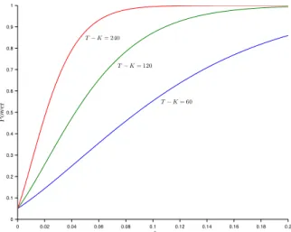
In Figure 2, we present the power of the F-test as a function of ω∗ =
T ω/(T−K−1) forT−K= 60, 120, and 240, when the size of the test is 5%. It shows that the power function of theF-test is an increasing function ofT−Kandω∗ and this allows us to determine what level ofω∗ that we need to reject the null hypothesis with a certain probability. For example, if we wish the F-test to have at least a 50% probability of rejecting the
spanning null hypothesis, then we need ω∗ to be greater than 0.089 for
T−K= 60, 0.043 forT−K= 120, and 0.022 forT−K= 240.
Note thatω is the sum of two terms. The first term measures how close
theex anteglobal minimum-variance portfolios of the two frontiers are in terms of the reciprocal of their variances. The second term measures how close the ex ante tangency portfolios of the two frontiers are in terms of the square of the slope of their tangent lines.
In determining the power of the test, the distance between the two global minimum-variance portfolios is in practice a lot more important than the distance between the two tangency portfolios. We provide an example
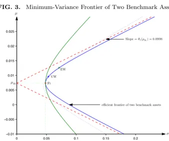
to illustrate this. Consider the case of two benchmark assets (i.e., K =
2), chosen as the equally weighted and value-weighted market portfolio of
the NYSE.14 Using monthly returns from 1926/1–2006/12, we estimate ˆµ
1 and ˆV11 and we have ˆµg1 = ˆb1/cˆ1 = 0.0074, ˆσg1 = 1/
√
ˆ
c1 = 0.048, and ˆ
θ1(ˆµg1) = 0.0998. We plot the ex postminimum-variance frontier of these
two benchmark assets in Figure 3. Suppose we take this frontier as theex antefrontier of the two benchmark assets and consider the power of theF -test for two different cases. In the first case, we consider a -test asset that slightly reduces the standard deviation of the global minimum-variance portfolio from 4.8%/month to 4.5%/month. This case is represented by the dotted frontier in Figure 3. Although geometrically this asset does not improve the opportunity set of the two benchmark assets by much, the
ω for this test asset is 0.1610 (with 0.1574 coming from the first term). Based on Figure 2, this allows us to reject the null hypothesis with a 79% 13The derivation of this expression is similar to that of (37) and therefore not provided. 14This example was also used by Kandel and Stambaugh (1989).
FIG. 2. Power Function of Mean-Variance Spanning Test with Single Test Asset 0 0.02 0.04 0.06 0.08 0.1 0.12 0.14 0.16 0.18 0.2 0 0.1 0.2 0.3 0.4 0.5 0.6 0.7 0.8 0.9 1 ω∗ Pow er T−K= 60 T−K= 120 T−K= 240 FIGURE 2
Power Function of Mean-Variance Spanning Test with Single Test Asset The figure plots the probability of rejecting the null hypothesis of mean-variance spanning as a
function of!§for three diÆerent values ofT°K(the number of time series observations minus
the number of benchmark assets), when there is only one test asset and the size of the test is 5%.
The spanning test is anF-test, which has a centralF-distribution with 2 andT°K°1 degrees
of freedom under the null hypothesis, and has a noncentralF-distribution with 2 andT°K°1
degrees of freedom with noncentrality parameter (T°K°1)!§under the alternatives.
43
The figure plots the probability of rejecting the null hypothesis of mean-variance spanning as a function ofω∗ for three different values ofT −K (the number of time series observations minus the number of benchmark assets), when there is only one test asset and the size of the test is 5%. The spanning test is an F-test, which has a central F-distribution with 2
and T −K−1 degrees of freedom under the null hypothesis, and has a
noncentralF-distribution with 2 and T−K−1 degrees of freedom with
noncentrality parameter (T−K−1)ω∗ under the alternatives.
probability for T −K = 60, and the probability of rejection goes up to
almost one for T −K = 120 and 240. In the second case, we consider
a test asset that does not reduce the variance of the global minimum-variance portfolio but doubles the slope of the asymptote of the frontier from 0.0998 to 0.1996. This case is represented by the outer solid frontier in Figure 3. While economically this test asset represents a great improvement in the opportunity set, its ω is only 0.0299 and the F-test does not have much power to reject the null hypothesis. From Figure 2, the probability
of rejecting the null hypothesis is only 20% for T −K = 60, 37% for
T−K= 120, and 66% forT−K= 240.
It is easy to explain why theF-test has strong power rejecting the span-ning hypothesis for a test asset that can improve the variance of the global minimum-variance portfolio but little power for a test asset that can only improve the tangency portfolio. This is because the sampling error of the former is in practice much less than that of the latter. The first term ofω
involves c−c1= 10N+KV−11N+K−10KV11−11K which is determined by V
es-timates ofµ(see Merton (1980)), even a small difference incandc1can be detected and hence the test has strong power to reject the null hypothesis when c 6= c1. However, the second term of ω involves θ2(ˆµg1)−θ
2 1(ˆµg1),
which is difficult to estimate accurately as it is determined by bothµandV. Therefore, even when we observe a large difference in the sample measure ˆ
θ2(ˆµg
1)−θˆ
2
1(ˆµg1), it is possible that such a difference is due to sampling
errors rather than due to a genuine difference. As a result, the spanning test has little power against alternatives that only display differences in the tangency portfolio but not in the global minimum-variance portfolio.
FIG. 3. Minimum-Variance Frontier of Two Benchmark Assets
0 0.05 0.1 0.15 0.2 −0.01 −0.005 0 0.005 0.01 0.015 0.02 0.025 VW EW Slope =θ1(µg1) = 0.0998 µg1 g1 σ µ
efficient frontier of two benchmark assets
FIGURE 3
Minimum-Variance Frontier of Two Benchmark Assets
The figure plots the minimum-variance frontier hyperbola of two benchmark assets in the (æ, µ)
space. The two benchmark assets are the value-weighted (VW) and equally weighted (EW)
port-folios of the NYSE.g1is the global minimum-variance portfolio and the two dashed lines are the
asymptotes to the e±cient set parabola. The frontier of the two benchmark assets is estimated using monthly data from the period 1926/1–2006/12. The figure also presents two additional fron-tiers for the case that a test asset is added to the two benchmark assets. The dotted frontier is for a test asset that improves the standard deviation of the global minimum-variance portfolio from 4.8%/month to 4.5%/month. The outer solid frontier is for a test asset that does not improve the global minimum-variance portfolio but doubles the slope of the asymptote from 0.0998 to 0.1996.
44
The figure plots the minimum-variance frontier hyperbola of two bench-mark assets in the (σ, µ) space. The two benchmark assets are the
value-weighted (VW) and equally value-weighted (EW) portfolios of the NYSE. g1
is the global minimum-variance portfolio and the two dashed lines are the asymptotes to the efficient set parabola. The frontier of the two benchmark assets is estimated using monthly data from the period 1926/1–2006/12. The figure also presents two additional frontiers for the case that a test as-set is added to the two benchmark asas-sets. The dotted frontier is for a test asset that improves the standard deviation of the global minimum-variance portfolio from 4.8%/month to 4.5%/month. The outer solid frontier is for a test asset that does not improve the global minimum-variance portfolio but doubles the slope of the asymptote from 0.0998 to 0.1996.
3.2. Multiple Test Assets
The calculation for the power of the spanning tests is extremely difficult when N >1. For example, even though the F-test in (27) has a central
under the alternatives. To study the power of the three tests forN >1, we need to understand the distribution of the two eigenvalues,λ1 and λ2, of the matrix ˆHGˆ−1 under the alternatives. In this subsection, we provide first the exact distribution ofλ1 andλ2 under the alternative hypothesis, then a simulation approach for computing the power in small samples, and finally examples illustrating the power under various alternatives.
Denote ω1≥ω2 ≥0 the two eigenvalues ofHGˆ−1 where H = ΘΣ−1Θ0 is the population counterpart of ˆH. The joint density ofλ1 andλ2can be written as f(λ1, λ2) = e− T(ω1+ω2) 2 1F1 T −K+ 1 2 ; N 2; D 2, L(I2+L) −1 × N−1 4B(N, T−K−N) " 2 Y i=1 λ N−3 2 i (1 +λi)T−K2+1 # (λ1−λ2), (41)
for λ1 ≥ λ2 ≥ 0, where L = Diag(λ1, λ2), 1F1 is the hypergeometric function with two matrix arguments, andD= Diag(T ω1, T ω2). Under the null hypothesis, the joint density function ofλ1andλ2 simplifies to
f(λ1, λ2) = N−1 4B(N, T−K−N) "Y2 i=1 λ N−3 2 i (1 +λi)T−K2+1 # (λ1−λ2). (42) To understand why λ1 and λ2 are essential in testing the null hypothesis, note that the null hypothesisH0 : Θ = 02×N can be equivalently written
as H0 : ω1 =ω2 = 0. This is becauseHGˆ−1 is a zero matrix if and only ifH is a zero matrix, and this is true if and only if Θ = 02×N since Σ is
nonsingular. Therefore, tests of H0 can be constructed using the sample
counterparts ofω1 and ω2, i.e., λ1 andλ2. In theory, distributions of all functions ofλ1 and λ2 can be obtained from their joint density function (41). However, the resulting expression is numerically very difficult to evaluate under alternative hypotheses because it involves the evaluation of a hypergeometric function with two matrix arguments. Instead of using the exact density function of λ1 and λ2, the following proposition helps us to obtain the small sample distribution of functions of λ1 and λ2 by simulation.
Proposition 1. λ1 andλ2 have the same distribution as the
eigenval-ues of AB−1 where A
∼W2(N, I2, D) andB ∼W2(T −K−N + 1, I2),
independent ofA.
With this proposition, we can simulate the exact sampling distribution
matricesA andB from the noncentral and central Wishart distributions, respectively. In the proof of Proposition 1 (in the Appendix), we give details on how to do so by drawing a few observations from the chi-squared and the standard normal distributions.
Before getting into the specific results, we first make some general obser-vations on the power of the three tests. It can be shown that the power is a monotonically increasing function inT ω1andT ω2.15 This implies that, as expected, the power is an increasing functions ofT. The more interesting question is how the power is determined for a fixedT. For such an analysis, we need to understand what the two eigenvalues ofHGˆ−1,ω1andω2, rep-resent. The proof of Lemma 2 works also for the population counterparts of ˆH, so we can write H = ∆a ∆b ∆b ∆c = a−a1 b−b1 b−b1 c−c1 , (43) wherea=µ0V−1µ,b=µ0V−11N+K,c= 10N+KV−11N+K,a1=µ01V11−1µ1,
b1 = µ01V11−11K, and c1 = 10KV11−11K are the population counterparts of
the efficient set constants. Therefore, H is a measure of how far apart
theex anteminimum-variance frontier ofK benchmark assets is from the
ex anteminimum-variance frontier of allN +K assets. Conditional on a given value of ˆG, the further apart the two frontiers, the bigger theH, the bigger theω1andω2, and the more powerful the three tests. However, for a given value ofH, the power also depends on ˆG, which is a measure of the
ex postfrontier of K benchmark assets. The better is theex post frontier ofK benchmark assets, the bigger the ˆG, and the less powerful the three tests. This is expected because if ˆGis large, we can see from (18) that the estimates ofαandδwill be imprecise and hence it is difficult to reject the null hypothesis even though it is not true.
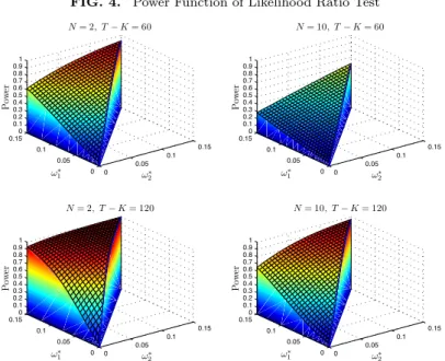
In Figure 4, we present the power of the likelihood ratio test as a function ofω∗1 =T ω1/(T −K−1) andω∗2 =T ω2/(T−K−1) forN = 2 and 10,
and for T −K = 60 and 120, when the size of the test is 5%. Figure 4
shows that for fixed ω∗1 and ω∗2, the power of the likelihood ratio test is an increasing function ofT −Kand a decreasing function ofN. The fact
that the power of the test is a decreasing function of N does not imply
we should use fewer test assets to test the spanning hypothesis. It only suggests that if the additional test assets do not increaseω1 andω2 (i.e., the additional test assets do not improve the frontier), then increasing the number of test assets will reduce the power of the test. However, if the 15It is possible for the Lagrange multiplier test that its power function is not
mono-tonically increasing inT ω1andT ω2when the sample size is very small. (See Perlman
(1974) for a discussion of this.) However, for the usual sample sizes and significance levels that we consider, this problem will not arise.
additional test assets can improve the frontier, then it is possible that the power of the test can be increased by using more test assets.
FIG. 4. Power Function of Likelihood Ratio Test
0 0.05 0.1 0.15 0 0.05 0.1 0.15 0 0.1 0.2 0.3 0.4 0.5 0.6 0.7 0.8 0.91 ω∗ 2 N= 2, T−K= 60 ω∗ 1 P ow er 0 0.05 0.1 0.15 0 0.05 0.1 0.15 0 0.1 0.2 0.3 0.4 0.5 0.6 0.7 0.8 0.91 ω∗ 2 N= 10, T−K= 60 ω∗ 1 P ow er 0 0.05 0.1 0.15 0 0.05 0.1 0.15 0 0.1 0.2 0.3 0.4 0.5 0.6 0.7 0.8 0.91 ω∗ 2 N= 2, T−K= 120 ω∗ 1 P ow er 0 0.05 0.1 0.15 0 0.05 0.1 0.15 0 0.1 0.2 0.3 0.4 0.5 0.6 0.7 0.8 0.91 ω∗ 2 N= 10, T−K= 120 ω∗ 1 P ow er FIGURE 4
Power Function of Likelihood Ratio Test
The figure plots the probability of rejecting the null hypothesis of mean-variance spanning as a function of!§
1and!2§using the likelihood ratio test when the size of the test is 5%, where (T°K°1)!§
1and (T°K°1)!§2are the eigenvalues of the noncentrality matrixT HGˆ°1. The four plots are for two diÆerent values ofN(number of test assets) and two diÆerent values ofT°K
(number of time series observations minus number of benchmark assets). The likelihood ratio test is anF-test, which has a centralF-distribution with 2Nand 2(T°K°N) degrees of freedom under the null hypothesis.
45
The figure plots the probability of rejecting the null hypothesis of mean-variance spanning as a function ofω∗
1 andω2∗using the likelihood ratio test when the size of the test is 5%, where (T−K−1)ω∗
1 and (T−K−1)ω2∗are the eigenvalues of the noncentrality matrixT HGˆ−1. The four plots are for two different values of N (number of test assets) and two different values
ofT−K (number of time series observations minus number of benchmark
assets). The likelihood ratio test is an F-test, which has a central F -distribution with 2N and 2(T−K−N) degrees of freedom under the null hypothesis.
The plots for the power function of the Wald and the Lagrange multiplier tests are very similar to those of the likelihood ratio test, so we do not report them separately. For the purpose of comparing the power of these three tests, we report in Table 2 the probability of rejection of the three
tests for N = 10 and T −K = 60 under different values of ω∗
1 and ω∗2. Although the difference in the power between the three tests is not large,
a pattern emerges. When ω2 ≈ 0, the Wald test is the most powerful
among the three. However, when ω1 ≈ ω2, the Lagrange multiplier test
is more powerful than the other two. There are only a few cases where the likelihood ratio test is the most powerful one. The pattern that we
which test is more powerful depends on the relative magnitude of ω1 and
ω2. The following lemma presents two extreme cases that help to identify alternative hypotheses withω2≈0 orω1≈ω2.
Lemma 3. Define µz= arg min r θ2(r)−θ12(r) = ∆b ∆c. (44)
Under alternative hypotheses, we have (i)ω2 = 0 if and only ifc=c1 or
θ2(µz) =θ2
1(µz), (ii) ω1=ω2 if and only if
c−c1 ˆ c1 = θ 2(µz) −θ2 1(µz) 1 + ˆθ2 1(µz) . (45)
The first part of the lemma suggests that when there is a point at which
the two ex ante minimum-variance frontiers are very close, then we have
ω2 ≈ 0. The second part of the lemma suggests that if the percentage
reduction of the inverse of the variance of the global minimum-variance portfolio is roughly the same as the percentage increase in one plus the square of the slope of the tangent line (when they-intercept of the tangent line isµz), then we will haveω1≈ω2.
As discussed earlier in the single test asset case, the effect of a small improvement of the standard deviation of the global minimum-variance portfolio is more important than the effect of a large increase in the slope of the tangent lines. Therefore, if we believe that the test assets could allow us to reduce the standard deviation of the global minimum-variance portfolio by even a small amount under the alternative hypothesis, then we should expectω1 to dominateω2 and the Wald test should be slightly more powerful than the other two tests.
4. A STEP-DOWN TEST
For reasonable alternative hypotheses, as shown earlier, the distance be-tween the standard deviations of the two global minimum-variance port-folios is the primary determinant of the power of the three spanning tests whereas the distance between the two tangency portfolios is relatively u-nimportant. This is expected because the test of spanning is a joint test of
α= 0N andδ= 0N and it weighs the estimates ˆαand ˆδaccording to their
statistical accuracy. Since δ does not involve µ (recall that δ is propor-tional to the weights of theN test assets in the global minimum-variance portfolio of all N +K assets), it can be estimated a lot more accurately than α. Therefore, tests of spanning inevitably place heavy weights on ˆδ
TABLE 2.
Comparison of Power of Three Tests of Spanning Under Normality
Likelihood Ratio Test
ω2∗= 0.0 ω∗2= 0.3 ω2∗= 0.6 ω∗2 = 0.9 ω2∗= 1.2 ω2∗= 1.5 ω∗1= 0.0 0.0500 ω∗1= 0.3 0.0823 0.1251 ω∗1= 0.6 0.1226 0.1752 0.2338 ω∗1= 0.9 0.1724 0.2307 0.2952 0.3612 ω∗1= 1.2 0.2260 0.2913 0.3596 0.4257 0.4913 ω∗1= 1.5 0.2834 0.3533 0.4228 0.4897 0.5533 0.6127 Wald Test ω2∗= 0.0 ω∗2= 0.3 ω2∗= 0.6 ω∗2 = 0.9 ω2∗= 1.2 ω2∗= 1.5 ω∗1= 0.0 0.0500 ω∗1= 0.3 0.0825 0.1243 ω∗1= 0.6 0.1241 0.1735 0.2292 ω∗1= 0.9 0.1739 0.2289 0.2901 0.3546 ω∗1= 1.2 0.2299 0.2905 0.3547 0.4193 0.4834 ω∗1= 1.5 0.2902 0.3538 0.4195 0.4829 0.5450 0.6042
Lagrange Multiplier Test
ω2∗= 0.0 ω∗2= 0.3 ω2∗= 0.6 ω∗2 = 0.9 ω2∗= 1.2 ω2∗= 1.5 ω∗1= 0.0 0.0500 ω∗1= 0.3 0.0820 0.1260 ω∗1= 0.6 0.1216 0.1754 0.2362 ω∗1= 0.9 0.1685 0.2314 0.2981 0.3650 ω∗1= 1.2 0.2199 0.2902 0.3617 0.4296 0.4962 ω∗1= 1.5 0.2731 0.3496 0.4234 0.4930 0.5589 0.6195
The table presents the probabilities of rejection of Wald, likelihood ratio, and La-grange multiplier tests of spanning in 100,000 simulations under the alternative hy-potheses when the number of test assets (N) is equal to 10 and the number of time series observations less the number of benchmark assets (T−K) is equal to 60. The size of the tests is set at 5% and the alternative hypotheses are summarized by two measuresω∗
1 andω2∗, where (T−K−1)ω1∗and (T−K−1)ω∗2 are the eigenvalues of
the noncentrality matrixT HGˆ−1. Numbers that are boldfaced indicate the test has
the highest power among the three tests.
and little weights on ˆα. Although this practice is natural from a statisti-cal point of view, it does not take into account the economic significance
of the departure from the spanning hypothesis. A small difference in the global minimum-variance portfolios, while statistically significant, is not necessarily economically important. On the other hand, a big difference in the tangency portfolios can be of great economic importance, but this importance is difficult to detect statistically.
The fact that statistical significance does not always correspond to e-conomic significance for the three spanning tests suggests that researchers need to be cautious in interpreting thep-values of these tests. A lowp-value does not always imply that there is an economically significant difference between the two frontiers, and a highp-value does not always imply that the test assets do not add much to the benchmark assets. To mitigate this problem, we suggest researchers should examine the two components of the spanning hypothesis (α= 0N and δ = 0N) individually instead of
joint-ly. Such a practice could allow us to better assess the statistical evidence against the spanning hypothesis.
To be more specific, we suggest the following step-down procedure to test the spanning hypothesis.16 This procedure is potentially more flexible and provides more information than the three tests discussed earlier.
The step-down procedure is a sequential test. We first test α = 0N,
and then testδ = 0N but conditional on the constraint α= 0N. To test α= 0N, similar to the GRSF-test, denote
F1= T−K−N N |Σ¯| |Σˆ|−1 ! = T−K−N N ˆ a−ˆa1 1 + ˆa1 , (46)
where ˆΣ is the unconstrained estimate of Σ and ¯Σ is the constrained
es-timate of Σ by imposing only the constraint of α = 0N. Under the null
hypothesis,F1has a centralF-distribution withN andT−K−N degrees of freedom. Now to testδ= 0N conditional α= 0N, we use the following F-test F2 = T −K−N+ 1 N |Σ˜| |Σ¯|−1 ! = T −K−N+ 1 N " ˆc+ ˆd ˆ c1+ ˆd1 ! 1 + ˆa1 1 + ˆa −1 # , (47)
where ˜Σ is the constrained estimate of Σ by imposing both the constraints
of α = 0N and δ = 0N. In the Appendix, we show that under the null
16See Section 8.4.5 of Anderson (1984) for a discussion of the step-down procedure.
It should be noted that the step-down procedure there applies to each of the test assets but not to each component of the hypothesis as in our case.
hypothesis, F2 has a central F-distribution with N and T −K−N + 1 degrees of freedom, and it is independent ofF1.
Suppose the level of significance of the first test is α1 and that of the
second test is α2. Under the step-down procedure, we will accept the
spanning hypothesis if we accept both tests. Therefore, the significance level of this step-down test is 1−(1−α1)(1−α2) = α1+α2−α1α2.17 There are two benefits of using this step-down test. The first is that we can get an idea of what is causing the rejection. If the rejection is due to the first test, we know it is because the two tangency portfolios are statistically very different. If the rejection is due to the second test, we know the two global minimum-variance portfolios are statistically very different. The second benefit is flexibility in allocating different significance levels to the two tests based on their relative economic significance. For example, knowing that it does not take a big difference in the two global minimum-variance portfolio to rejectδ= 0N at the traditional significance level of 5%, we may like to set α2to a smaller number so that it takes a bigger difference in the two global minimum-variance portfolios for us to reject this hypothesis. Contrary to the three traditional tests that permit the statistical accuracy of ˆαand ˆδto determine the relative importance of the two components of the hypothesis, the step-down procedure could allow us to adjust the significance levels based on the economic significance of the two components. Such a choice could result in a power function that is more sensible than those of the traditional tests.
To illustrate the step-down procedure, we return to our earlier example of two benchmark assets in Figure 3. ForT−K= 60 and a level of signif-icance of 5%, we show that the three traditional tests reject the spanning hypothesis with probability 0.79 for a test asset that merely reduces the standard deviation of the global minimum-variance portfolio from 4.8% to 4.5%, whereas for a test asset that doubles the slope of the asymptote from 0.0998 to 0.1996, the three tests can only reject with probability 0.20. In Table 3, we provide the power function of the step-down test for these two cases, using different values of α1 and α2 while keeping the significance level of the test at 5%.18 For different values ofα
1and α2, the step-down test has different power in rejecting the spanning hypothesis. However, in order for the step-down test to be more powerful in rejecting the test asset that doubles the slope of the asymptote, we need to setα2to be less than 0.0001. Note that if we wish to accomplish roughly the same power as the traditional tests, all we need to do is to set α1 = α2 = 0.02532. While
17Alternatively, one can reverse the order by first testing δ= 0
N and then testing α= 0N conditional onδ= 0N. In choosing the ordering of the tests, the natural choice is to test the more important component first.
18Under the alternative hypotheses, F
1 andF2 are not independent. Details on the
choosing the appropriate α1 and α2 is not a trivial task, it is far better to be able to have control over them than to leave them determined by statistical considerations alone.
TABLE 3.
Power of Step-Down Test of Spanning Under Normality
Probability of Rejection Significance Levels ∆a= 0.0299 ∆a,∆b= 0 α1 α2 ∆b,∆c= 0 ∆c= 67.16 0.00000 0.05000 0.05117 0.87457 0.02532 0.02532 0.19930 0.80914 0.04040 0.01000 0.23996 0.70256 0.04905 0.00100 0.25889 0.42230 0.04914 0.00090 0.25908 0.41071 0.04924 0.00080 0.25927 0.39798 0.04933 0.00070 0.25946 0.38385 0.04943 0.00060 0.25966 0.36794 0.04952 0.00050 0.25985 0.34971 0.04962 0.00040 0.26004 0.32829 0.04971 0.00030 0.26023 0.30217 0.04981 0.00020 0.26041 0.26823 0.04990 0.00010 0.26060 0.21800 0.04995 0.00005 0.26070 0.17710 0.04996 0.00004 0.26071 0.16578 0.04997 0.00003 0.26073 0.15240 0.04998 0.00002 0.26075 0.13574 0.04999 0.00001 0.26077 0.11254 0.05000 0.00000 0.26068 0.05000
The table presents the probabilities of rejection of step-down test for two different alternatives, conditional on the frontier of two benchmark assets is given in Figure 3. The first alternative (∆a= 0.0299) is a test asset that doubles the slope of the asymptote to the efficient hy-perbola of the two benchmark assets. The second al-ternative (∆c= 67.16) is a test asset that reduces the standard deviation of the global minimum-variance port-folio of the two benchmark assets from 4.8%/month to 4.5%/month. The step-down test is a sequential test. The first test is anF-test onα = 0N and the second test is anF-test ofδ = 0N conditional on the restric-tion ofα= 0N. The null hypothesis of spanning is only accepted if we accept both tests. α1 and α2 are the
significance levels for the first and the second F-test, respectively. The number of time series observations is 62.
5. TESTS OF MEAN-VARIANCE SPANNING UNDER NONNORMALITY
5.1. Conditional Homoskedasticity
Exact small sample tests are always preferred if they are available. The normality assumption is made so far to derive the small sample distribu-tions. These results also serve as useful benchmarks for the general non-normality case. In this section, we present the spanning tests under the assumption that the disturbancetin (9) is nonnormal. There are two cas-es of nonnormality to consider. The first case is whentis nonnormal but it is still independently and identically distributed when conditional onR1t.
The second case is when the variance oftcan be time-varying as a function ofR1t, i.e., the disturbancet exhibits conditional heteroskedasticity.
For the first case thatt is conditionally homoskedastic, the three tests, (23)–(26), are still asymptotically χ2
2N distributed under the null
hypoth-esis, but their finite sample distributions will not be the same as the ones presented in Section II. Nevertheless, those results can still provide a very good approximation for the small sample distribution of the nonnormality case. To illustrate this, we simulate the returns on the test assets under
the null hypothesis but with t independently drawn from a multivariate
Student-tdistribution with five degrees of freedom.19 In Table 4, we present the actual probabilities of rejection of the three tests in 100,000 simulation-s, for different values ofK,N, andT, when the rejection decision is based on the 95th percentile of the exact distribution under the normality case.
As we can see from Table 4, even whent departs significantly from
nor-mality, the small sample distribution derived for the normality case still works amazingly well. Our findings are very similar to those of MacKinlay
(1985) and Zhou (1993), in which they find that when t is conditionally
homoskedastic, nonnormality of t has little impact on the finite sample
distribution of the GRS test even for T as small as 60. Therefore, if one believes conditional homoskedasticity is a good working assumption, one should not hesitate to use the small sample version of the three tests
de-rived in Section II even though t does not have a multivariate normal
distribution.20
5.2. Conditional Heteroskedasticity
When t exhibits conditional heteroskedasticity, the earlier three test
statistics, (23)–(26), will no longer be asymptoticallyχ2
2N distributed under
19Due to the invariance property, it can be shown that the joint distribution ofλ 1
andλ2does not depend on Σ whent has a multivariate elliptical distribution. Details are available upon request.
20For some distributions of
t, Dufour and Khalaf (2002) provide a simulation based method to construct finite sample tests in multivariate regressions. Their methodology can be used to obtain exact tests of spanning under multivariate elliptical errors.
TABLE 4.
Sizes of Small Sample Tests of Spanning Under Nonnormality of Residuals
Actual Probabilities of Rejection
K N T W LR LM 2 2 60 0.048 0.048 0.048 120 0.049 0.050 0.050 240 0.051 0.051 0.051 10 60 0.047 0.047 0.047 120 0.046 0.046 0.046 240 0.047 0.049 0.050 25 60 0.046 0.047 0.047 120 0.046 0.046 0.046 240 0.047 0.048 0.048 5 2 60 0.049 0.048 0.048 120 0.051 0.051 0.051 240 0.051 0.051 0.051 10 60 0.047 0.047 0.047 120 0.048 0.048 0.048 240 0.049 0.049 0.048 25 60 0.046 0.046 0.047 120 0.046 0.046 0.046 240 0.048 0.048 0.048 10 2 60 0.050 0.049 0.049 120 0.049 0.049 0.049 240 0.051 0.051 0.051 10 60 0.048 0.048 0.048 120 0.049 0.049 0.049 240 0.049 0.049 0.049 25 60 0.048 0.048 0.048 120 0.047 0.047 0.047 240 0.047 0.047 0.047
The table presents the probabilities of rejection of Wald (W), like-lihood ratio (LR), and Lagrange multiplier (LM) tests of spanning under the null hypothesis when the residuals follow a multivariate Student-tdistribution with five degrees of freedom. The rejection decision is based on 95th percentile of their exact distributions un-der normality and the results for different values of the number of benchmark assets (K), test assets (N), and time series observa-tions (T) are based on 100,000 simulations.
the null hypothesis.21 In this case, Hansen’s (1982) GMM is the common
21It can be shown that under the null hypothesis, the asymptotic distribution of the
three test statistics is a linear combination of 2N independentχ2
viable alternative that relies on the moment conditions of the model. In this subsection, we present the GMM tests of spanning under the regression approach. This is the approach used by Ferson, Foerster, and Keim (1993).
Define xt = [1, R0
1t]0, t=R2t−B0xt, the moment conditions used by
the GMM estimation ofB are
E[gt] =E[xt⊗t] = 0(K+1)N. (48)
We assumeRtis stationary with finite fourth moments. The sample
mo-ments are given by
¯ gT(B) = 1 T T X t=1 xt⊗(R2t−B0xt) (49)
and the GMM estimate of B is obtained by minimizing ¯gT(B)0S−1
T ¯gT(B)
where ST is a consistent estimate of S0 =E[gtgt0], assuming serial
uncor-relatedness ofgt. Since the system is exactly identified, the unconstrained estimate ˆB, and hence ˆΘ, does not depend onST and remains the same as their OLS estimates in Section II. The GMM version of the Wald test can be written as Wa=Tvec( ˆΘ0)0[(AT ⊗IN)ST(A0T ⊗IN)]− 1 vec( ˆΘ0)∼Aχ22N, (50) where AT = 1 + ˆa1 −µˆ1Vˆ11−1 ˆb1 −10 KVˆ− 1 11 . (51)
Since both the model and the constraints are linear, Newey and West (1987) show that the GMM version of the likelihood ratio test and the Lagrange multiplier test have exactly the same form as the Wald test, even though one needs the constrained estimate of B to calculate the likelihood ratio and Lagrange multiplier tests. Therefore, all three tests are numerically identical if they use the sameST. In practice, different estimates ofST are often used for the Wald test and the Lagrange multiplier test. For the case
of the Wald test, ST is computed using the unconstrained estimate of B
whereas for the Lagrange multiplier test,ST is usually computed using the
constrained estimate of B. Since the constrained estimate of B depends
on the choice of ST, a two-stage or an iterative approach is often used
for performing the Lagrange multiplier test. Despite using different ST, the two tests are still asymptotically equivalent under the null hypothesis. For the rest of this section, we focus on the GMM Wald test because its analysis does not require a specification of the initial weighting matrix and the number of iterations.
5.3. A Specific Example: Multivariate Elliptical Distribution To study the potential impact of conditional heteroskedasticity on test-s of test-spanning, we look at the catest-se that the returntest-s have a multivariate elliptical distribution. Under this class of distributions, the conditional variance oftis in general not a constant, but a function ofR1t, unless the
returns are multivariate normally distributed. The use of the multivariate elliptical distribution to model returns can be motivated both empirically and theoretically. Empirically, Mandelbrot (1963) and Fama (1965) find that normality is not a good description for stock returns because stock returns tend to have excess kurtosis compared with the normal distribu-tion. This finding has been supported by many later studies, including Blatteberg and Gonedes (1974), Richardson and Smith (1993) and Zhou (1993). Since many members in the elliptical distribution like the multi-variate Student-t distribution can have excess kurtosis, one could better capture the fat-tail feature of stock returns by assuming that the returns follow a multivariate elliptical distribution. Theoretically, we can justify the choice of multivariate elliptical distribution because it is the largest class of distributions for which mean-variance analysis is consistent with expected utility maximization.
For our purpose, the choice of multivariate elliptical distribution is ap-pealing because the GMM Wald test has a simple analytical expression in this case. This analytical expression allows for simple analysis of the GMM Wald tests under conditional heteroskedasticity. The following proposition summarizes the results.22
Proposition 2. SupposeRtis independently and identically distributed
as a non-degenerate multivariate elliptical distribution with finite fourth moments. Define its kurtosis parameter as
κ=E[((Rt−µ)
0V−1(Rt−µ))2]
(N+K)(N+K+ 2) −1. (52)
Then the GMM Wald test of spanning is given by Wae=Ttr( ˆHGˆ−a1)
A
∼χ22N, (53)
whereHˆ defined in (22) and
ˆ Ga= " 1 + (1 + ˆκ)ˆa1 (1 + ˆκ)ˆb1 (1 + ˆκ)ˆb1 (1 + ˆκ)ˆc1 # , (54)
22We thank Chris Geczy for suggesting the use of kurtosis parameter in this
proposi-tion. See Geczy (1999) for a similar conditional heteroskedasticity adjustment for tests of mean-variance efficiency under elliptical distribution.