From spline wavelet to sampling theory on circulant graphs and beyond– conceiving sparsity in graph signal processing

(1)

Imperial College London

Department of Electrical and Electronic Engineering

Communication and Signal Processing Group

From Spline Wavelet to Sampling Theory

on Circulant Graphs and Beyond–

Conceiving Sparsity in Graph Signal Processing

Madeleine S. Kotzagiannidis

(2)

(3)

Declaration of Originality

I herewith certify that this thesis, and the research it comprises, are the product of my own work. Any ideas or quotations from the work of other people, published or otherwise, are fully acknowledged in accordance with the standard referencing practices of the discipline. The material of this thesis has not been submitted for any degree at any other academic or professional institution.

(4)

(5)

(6)

(7)

Copyright Declaration

The copyright of this thesis rests with the author and is made available under a Creative Commons Attribution Non-Commercial No Derivatives licence. Researchers are free to copy, distribute or transmit the thesis on the condition that they attribute it, that they do not use it for commercial purposes and that they do not alter, transform or build upon it. For any reuse or redistribution, researchers must make clear to others the licence terms of this work.

(8)

(9)

Abstract

Graph Signal Processing (GSP), as the field concerned with the extension of classical signal processing concepts to the graph domain, is still at the beginning on the path toward providing a generalized theory of signal processing. As such, this thesis aspires to conceive the theory ofsparse representations on graphs by traversing the cornerstones of wavelet and sampling theory on graphs.

Beginning with the novel topic of graph spline wavelet theory, we introduce families of spline and e-spline wavelets, and associated filterbanks on circulant graphs, which lever-age an inherent vanishing moment property of circulant graph Laplacian matrices (and their parameterized generalizations), for the reproduction and annihilation of (exponen-tial) polynomial signals. Further, these families are shown to provide a stepping stone to generalized graph wavelet designs with adaptive (annihilation) properties. Circulant graphs, which serve as building blocks, facilitate intuitively equivalent signal processing concepts and operations, such that insights can be leveraged for and extended to more complex scenarios, including arbitrary undirected graphs, time-varying graphs, as well as associated signals with space- and time-variant properties, all the while retaining the focus on inducing sparse representations.

Further, we shift from sparsity-inducing to sparsity-leveraging theory and present a novel

sampling and graph coarsening framework for (wavelet-)sparse graph signals, inspired by Finite Rate of Innovation (FRI) theory and directly building upon (graph) spline wavelet theory. At its core, the introduced Graph-FRI-framework states that anyK-sparse signal residing on the vertices of a circulant graph can be sampled and perfectly reconstructed from its dimensionality-reduced graph spectral representation of minimum size 2K, while the structure of an associated coarsened graph is simultaneously inferred. Extensions to arbitrary graphs can be enforced via suitable approximation schemes.

Eventually, gained insights are unified in a graph-based image approximation framework which further leverages graph partitioning and re-labelling techniques for a maximally sparse graph wavelet representation.

(10)

(11)

Acknowledgements

I would like to thank my supervisor, Prof. Pier Luigi Dragotti. In addition, I would also like to thank the Department of Electrical and Electronic Engineering for providing the scholarship that facilitated this research.

I am grateful to my friends in London and beyond, who made these past four years an enjoyable experience, and at last and most of all, to my mom and dad, for their endless love and support in all of my projects.

(12)

(13)

List of Tables

3.1 Continuous e-Spline and Graph e-Spline Definitions in Comparison. c2017 Elsevier Inc. . . 63 3.2 Condition Numbers of the GWTs. . . 74 4.1 Overview of Proposed GWTs. . . 111

(18)

(19)

List of Figures

1.1 Sparsity on Graphs: Theory and Applications. . . 28 2.1 Minnesota Traffic Graph with Graph Signal in the (a) Vertex and (b)

Spec-tral Domain. The color bar in (a) describes the intensity values of the signal on the graph. . . 39 2.2 Circulant Graphs with generating setsS={1},S ={1,2}, and S={1,3}

(from left). c2017 Elsevier Inc. . . 44 3.1 Localization of the HGSWT filters for k = 2 in the graph vertex domain

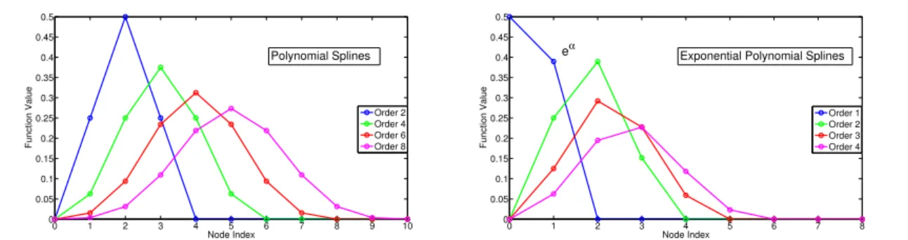
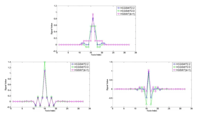
for circulantGwithS ={1,2}: shown at vertexv= 5∈V onG(left), and corresponding graph filter functions at alternate vertices. c2017 Elsevier Inc. . . 53 3.2 Classical Discrete Polynomial and Exponential Splines. . . 61 3.3 The HGSWT filter functions at k = 1 for different bipartite circulant

graphs,N = 16. c2017 Elsevier Inc. . . 62 3.4 The HGESWT filter functions (k = 1) for different bipartite circulant

graphs at α= 2_Nπ,N = 16. c2017 Elsevier Inc. . . 63 3.5 Comparison of NLA (lower left) and denoising performance (lower right)

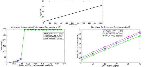
for a linear polynomial (top). . . 73 3.6 Comparison of NLA (lower left) and denoising performance (lower right)

for a linear polynomial (top) on a circulant graph withS = (1,2,3,4). . . . 74 3.7 Comparison of NLA (lower left) and denoising performance (lower right)

for a sinusoidal with (α= 2_Nπ4) (top). . . 75 3.8 Comparison of NLA (lower left) and denoising performance (lower right)

for a sum of sinusoidals with (α1 = 2_Nπ1,α2 = 2_Nπ5) (top). c2017 Elsevier

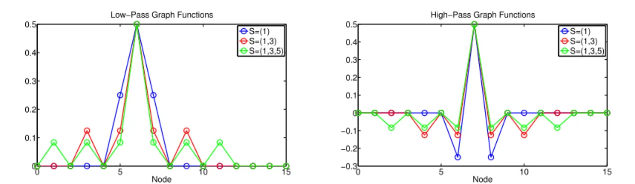
Inc. . . 76 3.9 Comparison of Graph-filter functions: analysis low-pass (top), synthesis

low-and high-pass (from left) at one level for the linear spline constructions on the graph withS = (1,2). . . 76 3.10 Comparison of Graph-filter functions: analysis low-pass (top), synthesis

low-and high-pass (from left) at one level for the linear spline constructions on the graph withS = (1,2,3,4). . . 77

(20)

LIST OF FIGURES

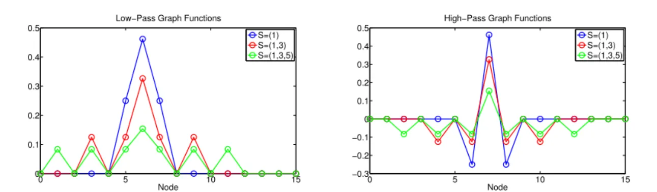
3.11 Comparison of Graph-filter functions: analysis low-pass (top), synthesis low-and high-pass (from left) at one level for the convolved e-spline

con-structions on the graph withS = (1,2). . . 77

4.1 Piecewise Smooth Graph Signal on a Circulant Graph. . . 86

4.2 Illustrative Time-Varying-Graph att= 0,1,2. . . 89

4.3 Walk across two circulant graphs. . . 91

4.4 Graph Cartesian Product of two unweighted circulant graphs. c2017 El-sevier Inc. . . 100

4.5 Graph Downsampling and Coarsening of G in Fig 4.4 on G2 w. r. t. s = 1∈S2 with coarsened ˜G2. c2017 Elsevier Inc. . . 103

4.6 Non-linear Approximation Performance Comparison for a piecewise smooth signal (top) on a toroidal graph product (left). . . 108

4.7 Non-linear Approximation Performance Comparison for a noisy piecewise smooth signal (top) on a circulant graph with bandwidthM = 1,5,9 (from left). . . 109

4.8 Non-linear Approximation Performance Comparison for a noisy piecewise smooth signal (top) on a circulant graph with bandwidthM = 1,5,9 (from left). . . 110

5.1 Traditional Sampling Scheme. c2017 Elsevier Inc. . . 113

5.2 Graph Coarsening for a Circulant Graph withS={1,2,3}. c2017 Elsevier Inc. . . 122

5.3 Sampling Scheme with Preceding Sparsification Step and One Level of Coarsening. c2017 Elsevier Inc. . . 122

5.4 Graph Cartesian Product of two unweighted path graphs. c2017 Elsevier Inc. . . 128

5.5 GFRI-Scheme under Graph Perturbations. . . 130

5.6 Coefficient Matrix C under Perturbations (displayed in magnitude, scale-factor 10). . . 134

5.7 Reconstruction Performance on a Perturbed Simple Cycle (N = 256), for 100 randomly generated sparse signalsxl (K = 4, minimum separation of 3 between entries). c2015 IEEE . . . 135

6.1 Non-Linear Approximation Comparison for the 2D Haar, 2D Linear Spline and proposed Graph Wavelet Transform (GWT) with 5 levels at 5% of non-zero coef-ficients (f. left).. . . 138

6.2 Random Graph Signal (b) with corresponding Graph Adjacency Matrix (a) before and after ((c)−(d)) applying a simple sort (graph kernel as in Eq. (6.2), with thresholdT = 0.3). . . 145

(21)

6.3 OriginalG(N = 64) after thresholding of weights (a), after RCM relabelling (b), signalxbefore/after relabelling (c), multiscaleHGSWT representation (atk= 1) of x(in magnitude) on ˜G for 3 levels (d). c2017 Elsevier Inc. . 146 6.4 Comparison of NLA performance at 5 levels for a 64×64 image patch. . . . 147 6.5 Comparison of NLA performance at 5 levels for a 64×64 image patch. . . . 148 6.6 Localized Basis Functions of thesparseGWT(bil,RCM)depicted on selected

(nodes) pixels (b) of the original image patch. . . 149 6.7 Localized Basis Functions of the sparseGWT(I,sort) depicted on selected

(nodes) pixels (b) of the original image patch. . . 150 6.8 Comparison of NLA performance at 5 levels for a 64×64 image patch. . . . 151 6.9 Comparison of NLA performance at 5 levels for a 64×64 image patch. . . . 151 6.10 (a) Original 64×64 image patch, (b)-(c) Graph Cut Regions for 1 cut &

(d) Comparison of NLA performance. c2017 Elsevier Inc. . . 152 6.11 (a) Original 64×64 image patch, (b)−(e) Graph Cut Regions for 3 cuts &

(f) Comparison of NLA performance. . . 152 6.12 Denoising performance comparison for a 64×64 image patch. . . 153 6.13 Denoising performance comparison between BM3D and simple cycle GWT

(22)

(23)

Notation

Sets and Numbers

N Natural Numbers (not including 0)

Z Integers

Z≥0 Nonnegative Integers

R Real Numbers

C Complex Numbers

S={s_i}_i SetS with elementssi

S{ Complement of setS

¯

z, z∗ Complex Conjugate of z∈C

[a, b] Closed Interval: {x∈_R:a≤x≤b} (a, b) Open Interval: {x∈_R:a < x < b}

[a, b) Partially closed Interval: {x∈R:a≤x < b}

C∞([a, b]) space of infinitely differentiable continuous functions over [a, b] Cp([a, b]) space of continuous functions withp continuous derivatives over [a, b]

n mod N nmodulo N

(i+j)N i+j moduloN

f(t)≷a f(t)> aorf(t)< a, for functionf :R→Rand a∈R

Vectors and Matrices x∈_CN _(or_~_x_∈

CN) vector or discrete-time signal of dimensionN

x(i) or xi i-th entry of vector x ||x||₂ l2-norm of vectorx,||x||2= q PN i=1|xi|2 ||x||0 l0-pseudo-norm of vectorx,||x||0 = #{i:xi6= 0}

1N constant vector of 1’s of dimensionN

1S vector with 1’s on set (or interval)S and 0’s otherwise

ei unit vector withei(i) = 1 and ei(j) = 0, j 6=i, of dimensionN

δij Kronecker delta (0 if i6=j, 1 ifi=j)

(24)

Notation

Ai,j orA(i, j) entry of matrix A at position (i, j)

AT transpose of matrix A

AH Hermitian (or conjugate) transpose of matrix A

A−1 inverse of matrixA ||A||F Frobenius-norm of matrixA,||A||F = q PN i=1 PN i=1|Ai,j|2

IN identity matrix of dimension N×N

0N,N zero matrix of dimension N ×N

◦ Hadamard (entrywise) product

⊗ Kronecker (or tensor) product

Signal Processing Notation

x(t) continuous-time signal

f(t)∗g(t) continuous-time convolution: R_−∞+∞f(τ)g(t−τ)dτ

Graph Notation A adjacency matrix

D degree matrix

L graph Laplacian matrix

An normalized adjacency matrix: D−1/2AD−1/2 Ln normalized graph Laplacian matrix: D−1/2LD−1/2

d degree per node ˜

Lα (exponential) e-graph Laplacian matrix

(25)

Abbreviations

DFT Discrete Fourier Transform

FRI Finite Rate of Innovation

GSP Graph Signal Processing

GFT Graph Fourier Transform

GWT Graph Wavelet Transform

LSI Linear Shift-Invariant

SP Signal Processing

wlog without loss of generality

Proposed Graph Wavelet Transforms

HGSWT Higher-Order Graph Spline Wavelet Transform Thm. 3.1 (p. 52)

HGESWT Higher-Order Graph E-Spline Wavelet Transform Thm. 3.2 (p. 56)

HCGSWT Higher-Order Complementary Graph Spline Wavelet Transform Thm. 3.4 (p. 69)

HCGESWT Higher-Order Complementary Graph E-Spline Wavelet Transform Thm. 3.5 (p. 71)

HBGWT Higher-Order Bandlimiting Graph Wavelet Transform Cor. 4.1 (p. 82)

(26)

Chapter 1

Introduction

1.1 Motivation and Objectives

Graphs, as high-dimensional (and often sparse) dependency structures, have become an increasingly favorable tool for the representation and processing of large data, as exempli-fied by i. a. social, transportation and neuronal networks, primarily due to their potential to capture (geometric) complexity.

The appeal of operating with respect to data encapsulated within the higher-dimensional dependency structures of a graph lies not only in the potential for superior data repre-sentation and processing for real-world applications, but also emerges in the development of a comprehensive mathematical framework, which seeks to extend conventional signal processing concepts to the graph domain, thus naturally challenging the structural con-finement of existing frameworks and posing intriguing new questions.

The resultant field of Graph Signal Processing (GSP) can be characterized as the collec-tive of theoretical and experimental efforts toward a more generalized theory of Signal Processing (SP), which attempts to leverage the complex connectivity of graphs in order to facilitate more sophisticated processing of (high-dimensional) data beyond traditional methods. Nevertheless, the developed underlying theory is still in its infancy and there is a need for a thorough and rigorous theoretical foundation in order to fully comprehend and exploit the capabilities of networks.

A graph consists of a set of vertices and a set of edges, whose associated weights char-acterize the similarity between the two vertices they respectively connect. In its essence, GSP aspires to use graphs as data representations, whose specific connectivity and edge weights are imposed by or inferred from the problem and/or data at hand, while further instilling the notion of an associated graph signal, which maps the data to a finite sequence of samples such that each sample value corresponds to a vertex in the graph [1].

(27)

Chapter 1. Introduction

The inherent challenge of incorporating and interpreting newly arising data dependencies, while maintaining equivalencies to classical cases, has given rise to a variety of different approaches, borrowing notions from i. a. algebraic and spectral graph theory ([2], [3]), algebraic signal processing theory [4], and general matrix theory [5]; here, it has remained an open problem to link structural properties of signals and underlying graphs to properties of graph operators and/or arising transform coefficients [1]. Graph theory and linear algebra in particular create a productive interplay in that any graph can be represented by a matrix and thus be subjected to (and benefit from) purely linear algebraic results, while at the same time, any generic (square) matrix can be interpreted as the connectivity information of a network, facilitating a geometrically richer approach.

Under this theme, the present thesis aspires to conceive sparsity on graphs from a the-oretical perspective, which i. a. features the problem of identifying an optimal (graph-dependent) basis for the sparse representation of a graph signal. Having evolved from a central issue in the area of classical transform analysis, in light of newly arising data-dependencies that need to be accommodated and a plethora of techniques and inter-pretations targeted at variable and, usually application-driven, desirable properties, this problem remains largely unanswered from a theoretically rigorous perspective. Further, we delve into the topic of sampling sparse signals on graphs, before eventually tackling the problem of graph-based sparse image approximation. In the course of this conception, we create a bridge from spline wavelet to sampling theory on graphs, which further links to their traditional counterparts in signal processing, on the basis of circulant graphs. Notions of matrix-bandedness and graph-relabelling additionally play a crucial role. Sparse graph signals, characterized by a small number of non-zero values relative to the dimension of the graph, represent a scarcely studied area of GSP, in particular, it remains unexplored how a sparse representation can be induced via a valid graph operator with respect to the underlying connectivity of the graph, or put differently, what classes of signals can be perfectly annihilated on a graph beyond piecewise constant signals. At the same time, it is of interest to investigate how sparsity on graphs can be leveraged for dimensionality reduction of the signal and coarsening of the associated graph, i. a. for efficient data processing and storage.

The proposed theoretical analysis is primarily conducted in an effort to understand sparse graph signals in the light of the structure and connectivity of graphs and contribute to a more rigorous theoretical foundation of GSP, while simultaneously developing insight for possible applications, such as sparse signal- and image-approximation on graphs.

As will be revealed in subsequent chapters, the inherent polynomial and LSI (Linear Shift-Invariance) quality of circulants gives rise to a range of interesting mathematical properties which can be leveraged for drawing (intuitive) connections and extensions from SP to GSP (see Fig. 1.1). In particular, graph operators defined on circulant graphs can be

(28)

diagonal-1.2. Contributions and Outline of Thesis

Polynomial Splines

Figure 1.1: Sparsity on Graphs: Theory and Applications.

ized by the DFT-matrix, which is central to traditional SP, while being well characterized in the vertex as well as in the spectral graph domain as a result of the regularity of the graph. Fundamental mathematical properties of the circulant graph Laplacian matrix are detected and incorporated into novel generalized graph differencing operators, which give rise to basis functions that are structurally similar to the classical discrete (e-)splines, thereby inspiring the creation of multilevel wavelet transforms on circulant graphs. The inherent Fourier characterisation in the spectral graph domain is further leveraged in the problem of sampling sparse signals on circulant graphs. Inspired by classical Finite Rate of Innovation theory, the derived framework facilitates the perfect recovery of sparse signals from a dimensionality reduced spectral representation while simultaneously identifying an associated coarsened graph; this not only extends the classical framework to a broader class of signals defined on complex structures beyond the real line, but further charac-terises the sampled signal through a reduced graph which preserves essential properties of the original.

1.2 Contributions and Outline of Thesis

In the following, we present an outline of the thesis with its major contributions.

Chapter 2 provides an overview of the general landscape ofgraph signal processing, com-mencing with a brief discussion of the most notable works and contributions on traditional sparse signal processing, followed by basic definitions and concepts from linear algebra and spectral graph theory, which we will be making use of throughout. Subsequently, we pro-ceed to state the general problem context of GSP and underlying notions, along with an overview of recent contributions to wavelet and sampling theory on graphs, and concluding with a specialized review ofcirculant graphs.

In Chapter 3, we introducegraph spline wavelet theory on circulant graphs and present a range of properties and results that derive from the discovered vanishing moment property of the circulant graph Laplacian, while also drawing connections to traditional spline

(29)

the-Chapter 1. Introduction

ory. We develop novel families of wavelets and associated filterbanks for the analysis and representation of functions defined on circulant graphs, where we distinguish between the vertex domain-based graph spline and e-spline wavelet transforms, and the complemen-tary graph (e-)spline wavelet transforms (derived via spectral factorization), and discuss their properties and special cases. As such, the theory developed in Ch. 3 serves as the foundation for subsequent chapters and their contributions.

Chapter 4 seizes the main insights and derived properties of Chapter 3 and appropriates them forgeneralized wavelet design on arbitrary undirected graphs targeted at the broader class of (piecewise) smooth graph signals. The chapter begins with a review and analysis of a general graph wavelet transform, elucidating how the theory of Ch. 3 constitutes a special case for circulant graphs, and evolves into the derivation of further graph wavelet transforms for undirected graphs with distinct annihilation properties. These include the generalized bandlimiting, space-variant and time-variant graph wavelet transforms as well as the multi-dimensional graph wavelet transform defined on product graphs. Additional analysis of the condition number and sparsifying-level of derived constructions is con-ducted.

Chapter 5 tackles the problem ofsparse sampling on graphsby introducing the novel GFRI-framework on circulant graphs and beyond, inspired by traditional FRI theory and directly leveraging the developed graph spline wavelet theory. In particular, the perfect recovery of (wavelet-)sparse signals from a dimensionality-reduced representation is established, while an associated coarsened graph can be identified; properties and special cases are discussed, as well as extensions to multi-dimensional sampling, while generalizations to arbitrary graphs are enforced via suitable approximation schemes. At last, an alternative approach to the latter is explored in form of (noisy) sampling on circulant graphs with perturbations.

Eventually, Chapter 6 presents a novel graph-based image processing framework which employs image (graph) segmentation followed by a variable, sparsity-driven graph wavelet analysis step for images featuring distinct discontinuities or patterns. More precisely, cir-culant graph wavelets with variable localization properties are applied on approximations of the partitioned subgraphs, which represent image regions of homogeneous intensity con-tent. Further relevant performance-enhancing concepts such as the optimal graph labelling are discussed, while the superiority of the method compared to traditional tensor product wavelet bases is illustrated on the basis of real and artificial image patches. In essence, this final chapter is designed to unify and implement certain gained notions on the theory of GSP within the concrete application of image processing, thereby directly leveraging the main strength of GSP to capture, and operate with respect to, the inherent geometry of given (image) data.

(30)

1.3. Publications

1.3 Publications

The following papers in press ([6],[7]) and publications ([8], [9], [10], [11]) were produced over the course of the PhD studies, and are incorporated throughout this thesis, which is accordingly annotated in footnotes.

Journal Papers (in press)

1. M. S. Kotzagiannidis and P. L. Dragotti, ”Sampling and Reconstruction of Sparse Signals on Circulant Graphs - An Introduction to Graph-FRI,” Appl. Comput. Harmon. Anal. (2017), https://doi.org/10.1016/j.acha.2017.10.003, available on arXiV: http://arxiv.org/abs/1606.08085.

2. M. S. Kotzagiannidis and P. L. Dragotti, ”Splines and Wavelets on Circulant Graphs,” Appl. Comput. Harmon. Anal. (2017), https://doi.org/10.1016/j.acha.2017.10.002,

available on arXiV: http://arxiv.org/abs/1603.04917.

Conference Papers

3. M. S. Kotzagiannidis and P. L. Dragotti, ”The Graph FRI framework-Spline wavelet theory and sampling on circulant graphs,” in2016 IEEE International Conference on Acoustics, Speech and Signal Processing (ICASSP), Shanghai, China, March 2016, pp. 6375–6379.

4. M. S. Kotzagiannidis and P. L. Dragotti, ”Higher-order graph wavelets and sparsity on circulant graphs,” in SPIE Optical Engineering+ Applications. Wavelets and Sparsity XVI, vol. 9597. San Diego, USA: International Society for Optics and Photonics, 2015, pp. 95 971E–95 971E-9.

5. M. S. Kotzagiannidis and P. L. Dragotti, ”Sparse graph signal reconstruction on circulant graphs with perturbations,” in 10th IMA Conference on Mathematics in Signal Processing, Birmingham, UK, 2014.

6. M. S. Kotzagiannidis and P. L. Dragotti, ”Sparse graph signal reconstruction and image processing on circulant graphs,” in 2014 IEEE Global Conference on Signal and Information Processing (GlobalSIP), 2014, pp. 923–927.

(31)

Chapter 2

On Graphs and Sparsity: A Brief

Review

2.1 Sparse Signal Processing

The search for a signal representation that is efficient, and hencesparse, has been largely thematised in areas such as signal processing and computational harmonic analysis, with recent efforts merging and going beyond established notions. It is not the purpose of this thesis to provide a comprehensive review or detailed analysis of classical definitions and methods in the first place, except in order to specifically motivate a need for and/or draw comparisons to graph-based theory and methods, and as such, only its rough outlines will be retraced, whilst referring to more elaborate review works.

A vectorf ∈_RN _{is described as sparse if its}_l

0-pseudo-norm ||f||0 = #{i:fi 6= 0} is small

relative to the vector-dimensionN.

(Sparse) signal approximation in a given basis{un}Nn=0−1 is thus essentially conducted by

projecting a signal (or function)x∈_RN _{onto a small number} _{K << N} _{of suitable basis}

elements

x≈ X

n∈IK(x)

cnun.

The coefficients cn = ˜uTnx are obtained via the analysis with a (bi-)orthogonal basis

{u˜n}nN=0−1 and IK(x) denotes the set of K indices. In the case of linear approximations,

the latter are selected to correspond to fixed subspaces of lowest possible dimension, while non-linear approximations consider the best (signal-dependent) spaces, such as the atoms corresponding to the highest magnitude coefficients for the best K-term approximation, which take advantage of and capture i. a. some form of regularity of the signal as well as occurring localized discontinuities [12]. The latter, non-linear approach, in particular,

(32)

2.1. Sparse Signal Processing

signifies an increase in sparsity with more flexibility to achieve the best approximation. Notably, the discrete-time Fourier transform, as the basis of linear time-invariant operators with orthogonal atoms{un(x) =einx}n∈_Z, emerged as one of the earliest signal transforms

and gained popularity due to its particular efficiency in characterizing globally smooth sig-nals for i.a. denoising purposes, as an instance of linear approximation [13]. The Discrete Fourier Transform (DFT) nevertheless falls short of adequately (sparsely) describing sig-nals with arising discontinuities due to a lack of localization, and invites the approaches of bases with compact localized support, beginning with the Short Time Fourier Transform (STFT) or Gabor transform, which consists of windowed waveforms that can be applied locally, and culminating in the construction of multiscale wavelet transform bases, from the translations and dilations of localized low-frequency scaling functions and high-frequency mother wavelets, respectively providing a coarse approximation and detail preservation of the signal [13]. The class ofspline-wavelets, noted for their symmetry, regularity as well as localization and approximation properties for (piecewise) smooth functions, and char-acterized by synthesis functions which are higher-order polynomial splines, with variable design choices, including i.a. compact support (B-spline and biorthogonal spline wavelets), in particular emerged as superior [14].

In an effort to refine performance, wavelets have been further developed to incorporate adaptivity to more complex signal properties, such as orientation or translation-invariance at the sacrifice of critical sampling, in form of i.a. steerable [15] and stationary wavelet transforms [16]. Eventually, the sparse signal representation problem evolved into the task of selecting elements from a suitable dictionary, with a plethora of directions for the design and/or learning of overcomplete dictionaries, which may be analytic on the basis of mathematical functions, such as curvelets [17], contourlets [18] or bandelets [19], as well as directly extracted from data based on iterative training algorithms, such as the K-SVD algorithm [13]. Thereby, the former have i.a. tackled the problem of efficiently characteriz-ing higher-dimensional signals, such as images, which have one-dimensional, as opposed to zero-dimensional, smooth discontinuities that cannot be absorbed by traditional wavelet bases [20], via constructions that are more intricate than their predecessors; in particular, Chapter 6 will revisit this aspect through the conceptually simpler lens of graph theory. Moving from a domain which primarily targeted the creation of sparsity to another which specifically leverages it, we further consider sampling theory, as the bridge between discrete- and continuous-time signal processing, which has experienced a mathematical interplay with wavelet theory, and, specifically, the more recent advent ofsparse sampling

[21]. Sampling traditionally signifies the discretization of a continuous-time signal to a sequence of samples whose subsequent interpolation in turn generates a continuous signal. More generally, it denotes a dimensionality reduction in the discrete domain, such as that of a finite vector, followed by reconstruction or interpolation (a dimensionality increase),

(33)

Chapter 2. On Graphs and Sparsity: A Brief Review

and presents a relevant topic in the general investigation of sparsity on the real line, grids and ultimately graphs.

Traditionally, sampling theory and methods focus on the perfect reconstruction of a continuous-time signalx(t), which is typically filtered by a selected kernel ϕ(t) before be-ing uniformly sampled with a samplbe-ing periodT, from its samplesyn=hx(t), ϕ(t/T−n)i.

Its foundation is laid by the Nyquist-Shannon sampling theorem for bandlimited signals of the form

x(t) =X

k∈Z

xksinc(Bt−k)

with samplesxk =hBsinc(Bt−k), x(t)i and band [−B/2, B/2], which states a sufficient

condition for their perfect reconstruction at a sampling rate that is at least twice the maximum frequency ofB/2 [21]. Yet, it has been established that bandlimitedness is only a sufficient rather than necessary condition for perfect reconstruction.

Within a more comprehensive sampling framework, certain classes of signals have been identified, beyond the bandlimited or those confined to fixed subspaces, which possess a parametric representation with a finite number of degrees of freedom per unit of time, or Finite Rate of Innovation (FRI), of the form

x(t) = X k0_∈ Z K X k=1 xk0_,kg_k(t−t_k0) for known{g_k(t)}K

k=1, and free coefficients xk0_,k and time-shiftst_k0, and which can be ac-cordingly sampled and perfectly reconstructed, based on a spectral estimation scheme, known as the annihilating filter or Prony’s method [22], [23], [24]. One may choose from a range of different sampling kernels that satisfy the so-called Strang Fix condi-tions and their generalizacondi-tions [25], i.e. a linear combination of their shifted versions can reproduce polynomials or exponentials. The rate of innovation is then established as ρ= limτ→∞_τ1Cx −τ₂,τ₂

, with functionCx(ta, tb) counting the number of free parameters

over an interval [ta, tb] [22].

In particular, the sparsity of a signal consisting ofKDiracsx(t) =PK

k=1akδ(t−tk), t∈R

withtk∈[0, τ), is encapsulated in the parameter pairs (or innovations){ak, tk}K_k₌₁, which

completely determine the sampling rate of ρ = 2K/τ and signal, as for distinct tk, one

can retrievex(t) from 2K consecutive values of its transformed samplesτm=

P

ncm,nyn,

for a suitable choice of coefficients cm,n [22]. For instance, consider the samples yn =

x(t), ϕ _Tt −n

,n= 0, ..., N−1, obtained through filtering with a kernelϕ(t) of compact support that reproduces exponentials; that isϕ(t) satisfiesP

n∈_Zcm,nϕ(t−n) =eαmtfor a

proper choice of coefficientscm,n m= 0, ..., P, andαm∈C([26], [25]). Then the moments

take the form τm =PKk=1akeαm

tk

T, which corresponds to the Fourier transformation for

(34)

2.2. Graph Signal Processing

As will be enlarged upon in Chapter 5, the discrete matrix-based nature of the recon-struction approach, paired with a direct link to circularity in matrices (and hence graphs), facilitates its appropriation for and extension to the graph setting.

At last, due to our focus on sparse signals on graphs, a comparison with compressive sens-ing (CS) [27] is imperative. Accordsens-ing to CS theory, a sparse signalx∈RN can be

recov-ered with high probability from the dimensionality-reduced (sampled) signaly=Axunder suitable conditions on the rectangular sampling operator A∈_RM×N _with _{M << N} _and

sparsityK =||x||0, by solving an l1-minimization problem, or alternatively, using greedy

reconstruction algorithms [28]. While, in contrast to compressive sensing approaches [29], the recovery of the sparse vectorx in the previous scheme is exact at the critical dimen-sion of 2K measurements and based on a direct, spectral estimation technique, known as Prony’s method ([30], [22]), it should be noted that neither requires knowledge of the locations of the non-zero entries. Further, CS theory can be extended to the recovery of non-sparse signals x = Dc that have a sparse representation c in properly designed, overcomplete dictionariesD [31], which has also been addressed in the context of graphs by training a graph-based dictionary [32]. The sampling framework proposed in Chapter 5 envisions a similar approach in that smooth (wavelet-sparse) graph signalsxare filtered with a (circulant) multilevel graph wavelet transform in order to produce sparse signals

c which can subsequently be sampled; nevertheless, the recovery of x from c ultimately follows from the invertibility of the wavelet transform.

Contrary to the more recent learning- or optimization-driven approaches, this work pri-marily focuses on signal representations on graphs that are exactly sparse, following the derivation of suitable annihilating operators and wavelet transforms. Thereby, the no-tion of sparsity on graphs, and, in particular, how to induce a sparse representano-tion with respect to the graph connectivity, is conceived and developed on a fundamental level.

2.2 Graph Signal Processing

Motivated by the need for efficient and sophisticated data processing and representation, in light of the surge of available information in applications such as social, transportation or biological networks, as well as by the promise of developing a universal mathematical framework that goes beyond conventional signal processing, the field of Graph Signal Processing (GSP) emerged from a wide range of contributions, both novel and established. Some of the key challenges of this field comprise the identification and/or construction of the graph which captures the inherent geometry of a given data set (if not otherwise imposed by the application), the development suitable graph transforms which operate with respect to the graph structure as well as the application of powerful intuitions and techniques from traditional signal processing while simultaneously accommodating newly

(35)

arising data dependencies in the irregular graph domain.

At its core, GSP unifies basic concepts from algebraic and spectral graph theory with (computational) harmonic analysis [1], while linear algebra and convex optimization have gained an increasingly sustaining role. Spectral graph theory in particular has been in-strumental in extending mathematical concepts and intuitions from Fourier analysis to the graph domain, thereby introducing the notion of graph frequency spectra and graph Fourier transform bases. With the aim of establishing comparable SP properties, opera-tions and concepts in the graph domain, a breadth of intriguing GSP problems ranging from simple filtering operations up to more sophisticated constructions of graph wavelet fil-terbanks ([33], [34], [35], [36], [37]), graph signal interpolation and recovery ([38], [39], [40]), as well as applications encompassing graph-based image processing ([35], [41]), and semi-supervised learning ([42], [43]), have been derived in the wake of two elementary model assumptions for the central graph operator: the (positive semi-definite) graph Laplacian matrix, and the more generalized graph adjacency matrix. Whereas graph Laplacian-based approaches are focused on undirected graphs and leverage the associated convenient prop-erties of positive semi-definite matrices for spectral graph analysis, alternative avenues have featured both undirected and directed graph scenarios by resorting to the Jordan normal form of the adjacency matrix.

Apart from their suitability for clustering or filtering operations [1], graphs have further been employed for the dimensionality reduction of high-dimensional data sets to allow for localized operations on fewer graph vertices; diffusion maps in particular have been developed as a manifold learning technique with a random walk interpretation [44].

2.2.1 Graph Theory and Linear Algebra

A graphG= (V, E) is characterized by a set of verticesV ={0,1, ..., N−1}of cardinality |V|=N, and a set of edgesE ={e0, ..., eM−1}. Its underlying connectivity is captured in

an adjacency matrixA∈_RN×N _{with entries}

Ai,j =

(

wi,j >0, if nodesiand j are connected by an edge,(i6=j)

0, otherwise

for some non-zero weightwi,j and degree matrixD

Di,j =

(

di, ifi=j

(36)

with degreedi =P_jAi,j per nodei, which give rise to the non-normalized graph Laplacian

matrix

L=D−A.

As a fundamental graph matrix within both algebraic and spectral graph theory, the graph Laplacian has been subject to extensive investigation, with a number of results relating to its spectra [3], among others, and as such provides a key operator in the interpretation as well as implementation of classical signal processing concepts in the graph domain. Notably, when the graph is constructed via a kernel from a point cloud,L

can be interpreted as a second-order differential operator which, under certain conditions, converges to the Laplace-Beltrami differential operator on the underlying manifold [45]. The oriented (vertex-edge) incidence matrixS of an unweightedGdescribes the N ×M -matrix whose rows and columns are indexed by V and E respectively, i.e. its (i, j)-th entry is 1 (or −1) if edge ej originates (or terminates) at i; specifically, each edge of G

is assigned an orientation arbitrarily [46]. It is further related to the graph Laplacian via L = SST_{, both of which are of the same rank} _N ₋_k _for _k _{connected components,}

while for undirected graphs, its unoriented version with (0,1)-weights also exists [46]. For weighted graphs, equivalently, the incidence matrices are weighted and preceding statements continue to hold. The operation of ST _{on a real-valued function} _f _: _V _→

R

with value (STf)(e) takes the difference of f at the end-points of edgeein the manner of a discrete first-order differential operator [47]. The relation betweenST andL, and their differential counterparts, can be linked through a discrete version of Greens’s formula [47]. A graph whose vertices all have the same degree dis regular (or d-regular) which trans-lates to its graph adjacency and Laplacian matrix sharing the same eigenbasis V, with

A = VΓVH and L = dIN −A = V(dIN −Γ)VH. For irregular graphs, the

follow-ing relation can be established between the adjacency spectrum {γi}i and the maximum

degree per node: ¯d ≤ γmax ≤ dmax, with ¯d denoting the average degree per node and

equality γmax = dfor the d-regular case [48]. In graph theory, it has been of interest to

characterize special graph classes, such as paths, cycles or trees [2], which also extends to the probabilistic setting; the Erd˝os-R´enyi model, for instance, describes a popular process to generate random graphs G(n, p), from a fixed number n of vertices and probability p for the existence of an edge [49]. A relevant class is that of bipartite graphs, which are described by a vertex set V = X∪Y consisting of two disjoint sets X and Y, such that no two vertices within the same set are adjacent. Most prominently, the property that the eigenvalues of a bipartite graph adjacency matrix are symmetric with respect to zero [50], termed as thespectral foldingphenomenon, has motivated various GSP contributions, including perfect reconstruction graph filterbanks, sampling and approximation schemes ([35], [36]).

(37)

Further of interest is the symmetric normalized graph Laplacian Ln := D−1/2LD−1/2

with eigenvalues ˜λ ∈ [0 2), where ˜λmax = 2 if and only if the graph is bipartite. The

random-walk matrix ARW := D−1A denotes another well-known graph matrix, whose entriesARW_i,j represent the transition probability of going from vertexi toj on G, as one step of a Markov random walk.

In an effort to coin a broader class of graph matrices [47], thegeneralized graph Laplacian

(or discrete Schr¨odinger operator) ofGdefines a symmetric matrixM with entries

Mi,j =         

li,j, if nodesiand j are connected by an edge,(i6=j)

pi,i+li,i, (i=j)

0, otherwise

for weightsli,j and potentialpi,i; alternatively, it is given byM=L+Pfor graph Laplacian Land arbitrary diagonal matrix P.

Despite the fact that graph theory is generally concerned with the study of (pairwise) relations between objects and arising structures, it provides a substantial interplay with linear algebra in that any graph can be represented as a matrix and thus be subjected to (and benefit from) purely linear algebraic results, while at the same time, any generic (square) matrix can be interpreted as the connectivity information of a network, facili-tating a geometrically richer approach.1 Many insights in algebraic graph theory, encom-passing i.a. spectral graph theory, as the field of study focusing on the graph eigenvalues, hail from matrix theory, with the Perron-Frobenius Theorem for (symmetric) nonnegative irreducible matrices [47] playing a particularly crucial role. As will become evident, funda-mental results in this thesis employ the linear algebra perspective, notably when dealing with graph operators and transforms, nevertheless, specialized notions such as graph cuts and labelling are leveraged, all the while drawing connections to basic signal processing concepts.

2.2.2 The Basics of GSP

For the ensuing discussion, we mainly consider graphs, which are undirected, connected, (un-)weighted, and do not contain any self-loops. A graph signalxis traditionally a real-valued scalar function defined on the vertices of a graphG of dimensionN, with sample value x(i) at node i, and can be represented as the vector x ∈ _RN _{[1]; in this work, we}

extend this definition to include complex-valued graph signals x ∈ _CN_{, for illustration}

purposes, while maintaining real weights between connections on G. Time-periodic sig-nals have been commonly mapped to circular graphs, due to their sequential structure, but generally, signals can be represented on more complex graph structures, where edges

1

(38)

are not only used to invoke a sense of sequencing, but also i.a. similarity between sample values.

When G is undirected and connected, the graph Laplacian L is a positive semi-definite

matrix and has a complete set of orthonormal eigenvectors {ul}Nl=0−1, with corresponding

nonnegative eigenvalues 0 =λ0 < λ1 ≤ · · · ≤ λN−1, constituting a convenient property

that has facilitated key definitions and generalizing steps from traditional SP toward the field of GSP.

In particular, while the classical Fourier transform characterizes the expansion of a func-tionf ∈L2(R) ˆ f(ξ) :=hf, e2πiξti= Z R f(t)e−2πiξtdt (2.1)

in terms of the eigenfunctions of the 1-D Laplace operator −∆(·) =−∂2

∂t2, the definition

of an equivalent Graph Fourier Transform (GFT) ˆf of a (vectorized) function f residing on the vertices ofG, entails its representation in terms of the graph Laplacian eigenbasis

U = [u0| · · · |uN−1] such that ˆf = UHf, where H denotes the Hermitian transpose,

ex-tending the concept of the Fourier transform to the graph domain [1]. Its inverse is given byf(i) =PN−1

l=0 fˆ(λl)ul(i), with expansion coefficients

ˆ f(λl) :=hf,uli= N−1 X i=0 f(i)u∗_l(i). (2.2)

Emanating from the classical eigendecomposition of the Laplacian operator, the graph Laplacian spectrum of a connected graph carries a notion of frequency in that small eigenvalues correspond to eigenvectors that vary smoothly across the graph (thus directly reflecting its connectivity), while larger eigenvalues are associated with rapidly oscillating eigenvectors, justifying its ordering [1]. Here, the eigenvalueλ0= 0 is associated with the

all-constant u0 = √1_N and of multiplicity m0 = 1, signifying the number of its connected

components; alternatively, this is indicated by the so-called Fiedler value (or algebraic connectivity) of the form λ1 > 0 [51]. Nevertheless, the instance of a complete graph,

whose spectrum consists of only two values, presents a special case where large multiplici-ties can interfere with this conception of order and a more sophisticated theory is needed. Fig. 2.1 depicts a sample piecewise-constant graph signal on the unweighted Minnesota graph (from [52]), which has served as a common model for GSP contributions, both in the vertex and spectral domain.

A graph (wavelet) filter H in the vertex domain generally describes a linear transform which takes weighted averages (differences) of components of the input signalxat a vertex iwithin itsk-hop local neighborhoodN(i, k), given by ˜x(i) =Hi,ix(i) +Pj∈N(i,k)Hi,jx(j)

(39)

(a)

(b)

Figure 2.1: Minnesota Traffic Graph with Graph Signal in the (a) Vertex and (b) Spectral Domain. The color bar in (a) describes the intensity values of the signal on the graph.

for some coefficients{Hi,j}i,j,∈V; where applicable, it is expressed as a polynomial in the

graph Laplacian matrix H = h(L) = PN−1

k=0 hkLk for suitable hk (or alternatively, as a

polynomial in the adjacency matrix) [1]. The polynomial form is particularly favored for spectral domain design techniques since it simultaneously gives rise to an interpretation in the vertex domain.

Graph spectral filtering of a signalx∈_RN _{can be represented as ˜}_x₌_h₍_L₎_x_with

˜ x(i) = N−1 X l=0 ˆ x(λl)h(λl)ul(i) (2.3)

or equivalently through the GFT ˆx˜ = h(Λ)ˆx with ˆx˜(λl) = ˆx(λl)h(λl), where frequency

coefficients h(λl) are selected to attenuate or amplify certain frequency contributions.

Hence, when the spectral graph filter is given by a polynomialh(λl) = PKk=0hkλkl, it is

localized with respect to the vertex domain with

˜ x(i) = N−1 X j=0 x(j) K X k=0 hk(Lk)i,j, (2.4)

whereby the coefficients of the previous vertex-based transform can now be expressed as Hi,j =

PK

k=dG(i,j)hk(L)

k

i,j, with (Lk)i,j = 0 when the shortest-path distance dG(i, j)

between verticesi, j (minimum number of hops) is greater than k [37]. More specifically, a graph transform is said to be strictlyk-hop localized in the spatial domain of the graph if the filter coefficientsHi,j are zero beyond thek-hop neighborhood of each nodei. Other

classical signal processing notions such as convolution, translation or modulation can be similarly (directly or indirectly) generalized to the graph setting on the basis of the graph Laplacian eigenvectors [1].

(40)

Another line of work has sought to broaden the discussion to directed graphs by focusing on the properties of the graph adjacency matrix instead, deriving fundamental notions on frequency and sampling on the basis of its Jordan decomposition ([53], [54]).

Since the discussion in this thesis is largely focused on undirected graphs, most of the results can be easily adapted for different (properly normalized) graph matrices, however, for consistency, the graph Laplacian-based frequency (GFT) interpretation is adopted here.

2.2.3 Wavelets and Sparsity on Graphs

The notion of wavelets on graphs presents a promising avenue for the sophisticated analysis of complex data, which may be captured in form of a graph and underlying graph signal, beyond classical wavelet theory, due to the potential to operate with respect to the inherent geometry of the data in a more localised manner.

A range of designs have been proposed, notably including the diffusion wavelet [33], the biorthogonal and perfect reconstruction filterbank on bipartite graphs ([35], [36]), and the spectral graph wavelet [37], tailored to satisfy a set (or subset) of properties, which have evolved from the traditional domain, such as localization in the vertex or spectral graph do-main, critical sampling and invertibility, along with notions ofgraph-specific downsampling

andgraph-coarsening for a multiscale representation, as well as to facilitate generalizations to arbitrary graphs, for applications including image processing [1] and wavelet-regularized semi-supervised learning [55].

More specifically, the diffusion wavelets by Coifman and Maggioni [33] are orthogonalized basis functions based on compressed representations of (powers of) a diffusion operator, within a framework that is applicable to both graphs and smooth manifolds. The spectral graph wavelets by Hammond et al. [37] describe a class of wavelet operators which are constructed in the graph spectral domain of the graph Laplacian via dilations and transla-tions of a bandpass kernel. Further, the graph wavelet transform by Crovella and Kolaczyk (CKWT) [56] constitutes a multiscale design in the vertex domain (of unweighted graphs) based on the shortest-path distance; here, each wavelet is constant across vertices within a certain hop-neighborhood from the given center vertex.

A drawback of the aforementioned designs is their overcompleteness. This is remedied by i.a. lifting- [57] and tree-based [58] designs, as well as the graph wavelet filterbanks on bipartite graphs by Ortega et al. ([35], [36]). The latter in particular rely on con-venient properties of bipartite graphs which facilitate intuitive downsampling operations (by simply retaining either disjoint set) as well as a targeted design of spectral filters h(λ) for i.a. graph localization and compact support, following similar conditions as reg-ular domain (circulant)z-transformed filters, and can be generalized to arbitrary graphs

(41)

through a bipartite subgraph decomposition problem. In order to ensure that transforms are localized in the graph vertex domain, and can thus be expressed as polynomials of the graph Laplacian as well as provide efficient computation, some works employ a Cheby-chev approximation for designated kernels, incurring a small reconstruction error ([37], [35]). Further, the spline-like graph wavelet filterbanks on circulant graphs in [59], [34], [55], which are further detailed in the next section, describe vertex-localized transforms which similarly leverage mathematical properties of special graph classes for multiscale processing. For both the bipartite and circulant graph filterbanks, and contrary to tra-ditional signal processing notions, the low-and high-pass filtered content is retained by complementary sets of nodes.

While not necessarily of relevance to all of the above transforms, many of which are redun-dant, the problem of down-and upsampling a signal on the vertices of a graph is central to GSP, as the evolution of a key component of discrete multilevel signal transformations and filterbanks, and poses a particular challenge due to the complex connectivity of graphs. Along with it arises the problem of identifying acoarsened orreduced graph for subsequent multilevel operations, requiring a method of assigning suitable edges to a reduced set of vertices, while ensuring that certain properties of the original graph, among other desirable or essential ones, are preserved. Unless the graph at hand is highly structured or special, it remains unclear how to consistently extract a downsampling pattern and solution ap-proaches vary; for instance, in [60], it is proposed to select vertices based on the polarity of the components of the largest graph Laplacian eigenvector. Overall, it is usually desir-able to retain a representative half of the vertex set with connections between nodes in the retained as well as in the removed set being of relatively low weight [60]. Moreover, the coarsened graph should preserve essential graph connectivity properties of the original such as structure or sparsity, while being representative of the latter in both the vertex and spectral domain. These questions, among further GSP notions, are reviewed in i.a. [1], [60], while links between the problem of graph coarsening and the more established (approximate) graph coloring [61], which describes the search for a partition into vertex subsets of distinct color such that no two adjacent vertices share the same color, as well as to the dualspectral clustering [62], as the task of partitioning a (similarity) graph into clusters based on the graph Laplacian eigenvectors, have been discovered.

The topic of sparsity on graphs via wavelet analysis appears as a natural extension to its foundation in the discrete-time domain, and some works have opened its discussion through topics such as the wavelet coefficient decay at small scales of graph-regular sig-nals [63] via the spectral graph wavelet transform, the tight wavelet frame transform on graphs [64], as well as the overcomplete Laplacian pyramid transform with a spline-like in-terpolation step [60]. Nevertheless, such approaches so far lacked a concrete graph wavelet design methodology which targets the annihilation of graph signals, or, alternatively, the characterization of (classes of) graph signals which can be annihilated by existing

(42)

con-2.2. Graph Signal Processing

structions.

While established graph wavelet constructions, such as the spectral or tight graph wavelet ([37], [64]) may attain sufficiently (approximate) sparse graph wavelet domain represen-tations, i.a. for appropriate design choices of the associated wavelet kernel, there is no concrete (or intuitive) theory on what types of graph signals can be annihilated, beyond the class of piecewise-constant signals, in particular, based on the properties and connec-tivity of the graph at hand. Sparsity on graphs has been more tangibly addressed through the topic of dictionary learning on graphs [32], which considers the problem of identifying an (overcomplete) basisDunder which a given graph signalycan be sparsely represented asy=Dx. Accordingly, the work in this thesis breaks away from previous efforts, in that it examines how the connectivity of a graph can be leveraged to induce ‘exact’ sparsity in data on circulant graphs as well as more complex scenarios, beyond the intuitive example of the former.

2.2.4 Sampling on Graphs

Further, the topics of signal sampling and reconstruction on graphs have gained a growing interest within GSP, and in an effort to complement wavelet theory on graphs and provide context for the proposed bridge between wavelet and sampling theory, a brief overview of the latter is provided.

Signal recovery on graphs, constituting more broadly the empirical study as opposed to the analytical framework, has been tackled i.a. under the premise that the given signal is smooth with respect to the underlying graph, and may be formulated as an optimization problem within different settings ([40], [32]). In several works ([65], [66], [67], [68]), sam-pling theory for graphs, providing the specialized and more rigorous theorization of the former, is explored with predominant regard to the subspace of bandlimited graph sig-nals under different assumptions; specifically, Anis et al. [67] and Chen et al. [68] provide two alternative interpretations of bandlimitedness in the graph domain, where, in par-ticular, the latter employs matrix algebra to establish a linear reconstruction approach, based on a suitable choice of the retained (and known) sample locations. Moving be-yond the traditional domain, sampling theory in the context of graphs has furthermore attempted to address and incorporate graph coarsening, such as by Chen et al. in [68], also a problem in itself ([69], [70]), which bears the challenge of identifying a meaningful underlying graph for the sampled signal and has been generally featured to a lesser extent.

(43)

2.3 The Class of Circulant Graphs

Circulant graphs represent a special class of graphs that reveal a set of convenient prop-erties, which, not least of all, can be leveraged for the preservation of traditional signal processing concepts and operations. In particular, a circulant graph G is characterized by a generating set S = {s1, . . . , sM}, with 0< sk ≤ N/2, whose elements indicate the

existence of an edge between node pairs (i,(i±sk)N),∀sk∈S, where ()N is the modN

operation; more intuitively, a graph is circulant if its associated adjacency matrix is a cir-culant matrix under a particular node labelling [59] (see examples in Fig. 2.2). As part of a sub-class of circulant graphs, theM-connected ring graphGis defined via the generating setS={1, ..., M}, such that there exists an edge between nodesiand j, if (i−j)N ≤M

is satisfied; the associated circulant adjacency matrix is banded of bandwidth M. These graphs are i. a. utilized in the creation of small-world network graphs in the Watts-Strogatz model [71], prior to randomized edge rewiring, and can be embedded as tessellations in high-dimensional flat tori2 [72].

The eigenvalues of a circulant graph adjacency matrix of the form

C=           0 c1 · · · cN−2 cN−1 cN−1 0 . .. . .. cN−2 .. . ... . .. . .. ... c2 c3 . .. . .. c1 c1 c2 · · · 0          

are given byγj = 0 +c1ωj+c2ωj2+· · ·+cN−1ωjN−1, forωj =e−

i2πj

N , with a possible choice

of corresponding eigenvectorsvj = √1_N[1, ωj, ωj2, ..., ωN

−1

j ]T,j= 0, ..., N−1. The fact that

the graph Laplacian eigenbasis, or GFT, of a circulant graph can be represented by the DFT matrix reveals a first major link between classical and graph-based signal processing, since Fourier and frequency notions are indirectly upheld.

A circulant (adjacency) matrix is symmetric if its first row has the following structure C0,0:N−1 = [0 c1 c2 ... cN/2−1 cN/2 cN/2−1 ... c2 c1]; for an N ×N-matrix with N ∈ 2N,

this entails N/2 degrees of freedom (with c0 = 0, as we do not allow self-loops). Further

noteworthy about general (symmetric) circulant matrices in this context is the occurrence of eigenvalue multiplicities. While there is no general mathematical rule for the eigenvalue multiplicity distribution of a circulant (graph) matrix, with an arbitrary generating set, and it can only be determined by applying an exhaustive search approach, basic results on, for instance, the occurrence of odd and even multiplicities, such as in [73], can be inferred.

2

The analysis of data residing on general geometrical shapes, which can be described by meshes, in par-ticular, following the inference of corresponding graphs, can thus be conducted with graph-based methods.

(44)

2.3. The Class of Circulant Graphs

Figure 2.2: Circulant Graphs with generating sets S = {1}, S = {1,2}, and S ={1,3} (from left). c2017 Elsevier Inc.

Yet, the general intuition remains that a densely connected unweighted circulant graph is usually associated with large eigenvalue multiplicities, as evidenced by the complete graph of sizeN with adjacency spectrum consisting ofγ0=N −1 and γ1 =...=γN−1 =−1.

The symmetric, circulant graph Laplacian matrix L, with first row [l0 ... lN−1], can

be further defined through its so-called representer polynomial l(z) = PN−1

i=0 lizi with

z−j =zN−j, which bears a resemblance to the z-transform in SP. For the circulant per-mutation matrix Π with first row [0 1 0 ...], we obtain L = PN−1

i=0 liΠi. Every

cir-culant matrix is associated with a representer polynomial [74], which not only provides a means to accelerate circulant matrix multiplication, thereby unfolding an inherent poly-nomial quality of circulants, but also establishes a link to their spectral information. In particular, the polynomiall(z) of a circulant matrix L gives rise to its (unsorted) eigen-values3 via l(e2πikN ) = λ_k, k = 0, ..., N −1 [74]. This is not to be confused with its

characteristic polynomial, given bypL(x) = det(xIN −L) =QN_k₌₀−1(x−λk), which as the

unique monic polynomial of degree N vanishes at the eigenvalues λk, with determinant

detL=QN−1 k=0( PN−1 j=0 ω −j k lj) = QN−1

k=0 λk[74]. In fact, the roots ofpL(x) (eigenvalues ofL)

can be easily computed throughl(z); this has further inspired a method to solve polyno-mial equations by first finding a circulant matrix whose characteristic polynopolyno-mial matches the former and subsequently recovering the solutions through its representer polynomial ([75], [76]). As another consequence of their relation to polynomials, the product of cir-culant matrices can be computed by simply evaluating the product of their corresponding representer polynomials modulo the matrix dimension [77].

2.3.1 Downsampling and Reconnection on Circulant Graphs

Due to their regularity and structure, circulant graphs further lend themselves for defining meaningful downsampling operations in GSP. As established in [59] by Ekambaram et al., one can downsample a given graph signal by 2 on the vertices of G with respect to any

3

Hence, analogously to thez-transform which converts a discrete-time signal into a complex frequency domain representation, the circulant representer polynomial transfers the graph edge weight information to the spectral graph domain.

(45)

element sk ∈ S. In the simplest scenario, which will also be employed in this work, the

downsampling operation is conducted with respect to the outmost cycle (s1 = 1) of a given

circulant G, i.e. skipping every other labelled node, assuming that the graph at hand is connected such that s1 ∈S, and the dimension is N = 2n forn ∈N, the latter of which

facilitates a multiresolution analysis.

In addition, the same authors introduced a set of vertex-domain localized filters constitut-ing the ‘spline-like’ graph wavelet filterbank on circulant graphs ([34],[55]), which satisfies critical sampling and perfect reconstruction properties:

Theorem 2.1 ([34]). The set of low-and high-pass filters, defined on an undirected con-nected circulant graph with adjacency matrix A and degree d per node, take (weighted) averages and differences with respect to neighboring nodes at 1-hop distances of a given graph signal, and can be expressed as:

HLP = 1 2 IN + A d (2.5) HHP = 1 2 IN − A d . (2.6)

The filterbank is critically sampled and invertible as long as at least one node retains the low-pass component, while the complementary set of nodes retains the high-pass compo-nents.

The structure of the above filterbank motivated the families of graph spline wavelets which will be introduced in Chapter 3, and, as will be demonstrated, bear actual spline proper-ties4.

Multiscale analysis is conducted by iterating the result on the respective downsampled low-pass branches, in form of coarsened graphs, that may be obtained through suitable reconnection strategies [55]. In particular, this work will be primarily focused on critically-sampled filterbanks for which the critically-sampled output can be well-defined on (suitably) coars-ened graphs so as to control the problem dimensionality for multiscale analysis.

Succeeding the definition of a wavelet transform on a circulant graph, one thus needs to examine the problem of identifying suitable coarsened graph(s) on the vertices of which the downsampled low-(and high-)pass-representations of the original graph signal can be defined, as a means to facilitate the multiresolution decomposition in the graph domain. In general, it is not straightforward to determine if or how to reconnect the reduced set of vertices to form a coarsened graph, and the set of desired properties, comprising closure,

4

According to [55], the ‘spline-like’ filterbank of Theorem 2.1 derived its name from the linear spline FIR filters which are equivalent to the graph filters for a simple cycle graph, however, comparable properties are not mentioned for other graphs.