On Generalized Additive Models For Regression With Functional Data

ON GENERALIZED ADDITIVE MODELS FOR

REGRESSION WITH FUNCTIONAL DATA

A Dissertation

Presented to the Faculty of the Graduate School of Cornell University

in Partial Fulfillment of the Requirements for the Degree of Doctor of Philosophy

by

Mathew W. McLean August 2013

c

2013 Mathew W. McLean ALL RIGHTS RESERVED

ON GENERALIZED ADDITIVE MODELS FOR REGRESSION WITH FUNCTIONAL DATA

Mathew W. McLean, Ph.D. Cornell University 2013

The focus of this dissertation is the introduction of the functional generalized additive model (FGAM), a novel regression model for association studies between a scalar response and a functional predictor. The FGAM extends the commonly used functional linear model (FLM), offering greater flexibility while still being simple to interpret and easy to estimate. The link-transformed mean response is modelled as the integral with respect totofF{X(t), t}whereF(·,·) is an unknown, bivariate regression function andX(t) is a functional covariate. Compare this with the FLM which has F{X(t), t} =β(t)X(t), where β(t) is an unknown coefficient function. Rather than having an additive model in some projection of the data, the model incorporates the functional predictor directly and thus can be viewed as the natural functional extension of generalized additive models.

The first part of the dissertation shows how to estimate F(·,·) using tensor-product B-splines with roughness penalties. Fast, stable methods are used to fit the FGAM and I discuss how approximate confidence bands can be constructed for the true regression surface. Additional functional predictors can be included with little added difficulty. The performance of the estimation procedure and the confidence bands is evaluated using simulated data and I compare FGAM’s predic-tive performance with other competing scalar-on-function regression alternapredic-tives, including the popular functional linear model. I illustrate the usefulness of the approach through an application to brain tractography, where X(t) is a signal

from diffusion tensor imaging at position, t, along a tract in the brain. In one example, the response is disease-status (case or control) and in a second example, it is the score on a cognitive test. R code for performing estimation, plotting, and prediction for the FGAM is explained and is available in the package refund on CRAN.

Frequently in practise, only incomplete, noisy versions of the functions one wishes to analyze are observed. The estimation procedure used in the first part of the thesis requires that the functional predictors be noiselessly observed on a regular grid. In the second part of the dissertation, I restrict attention to the identity link-Gaussian error case and develop a Bayesian version of FGAM. This approach allows for the functional covariates to be sparsely observed and mea-sured with error. I consider both Monte Carlo and variational Bayes methods for jointly fitting the FGAM with sparsely observed covariates and recovering the true functional predictors. Due to the complicated form of the model posterior distri-bution and full conditional distridistri-butions, standard Monte Carlo and variational Bayes algorithms cannot be used. As such, the work should be of independent interest to applied Bayesian statisticians. The numerical studies demonstrate the benefits of the proposed algorithms over a two-step approach of first recovering the complete trajectories using standard techniques and then fitting a functional regression model. In a real data analysis, the methods are applied to forecasting closing price for items being auctioned on the online auction website eBay.

Finally, in the third part of the thesis I propose and compare several different procedures for testing when a scalar on function regression relationship is truly nonlinear. By using an alternative parametrization for the FGAM as a mixed model, it is shown how the functional linear model can be represented as a simple mixed model nested within the FGAM. Using this representation, I then consider

two types of tests, those based on restricted likelihood ratio tests for zero variance components in mixed models and those involving Bayes factors where we use gen-eralizations of g-priors as priors for the random effects coefficients. The methods are general and can also be applied to testing for interactions in a multivariate additive model or for testing for no effect in the functional linear model. The per-formance of the proposed tests is assessed on simulated data and in an application to measuring diesel truck emissions, where strong evidence of nonlinearities in the relationship between the functional predictor and the response are found.

BIOGRAPHICAL SKETCH

In west Philadelphia born and raised, on the playground was where I spent most of my days. Chilling out, maxing, relaxing all cool and all, shooting some b-ball outside of the school. When a couple of guys, who were up to no good, started making trouble in my neighbourhood. I got in one little fight and my mom got scared and said “You’re moving with your auntie and uncle in Bel-Air”.

Mathew William McLean has only spent one day in Philadelphia and never been to Bel-Air, but he did watch every episode of The Fresh Prince of Bel-Air while growing up in Winnipeg, Manitoba, Canada. He loved the long, freezing winters and short, mosquito-filled summers so much that he did not dare leave until his early twenties. It was at this time that the School of Operations Research and Information Engineering at Cornell University came calling, plucking him from his sheltered life of perpetual education in Winnipeg and transporting him to Ithaca, New York to continue the pursuit of his dream of never leaving school.

After five fun-filled years in Ithaca, Mr. McLean will be departing with a PhD and the promise of more schooling as a post-doctoral researcher at Texas A&M University in College Station, Texas.

To The Chapter House, thanks for all the pints.

To my friends,

ACKNOWLEDGEMENTS

I first wish to thank all the wonderful friends I have met during my time in graduate school who have made living in Ithaca such a pleasure these past five years. I was extremely lucky to have such an incredible group of people start the PhD program at the same time as me: Rolf, Martin, Brad, Shanshan, Zach, Dima, Tia, Gabriel, Yi, and Eric somehow managed to make being away from home and swamped with homework and exams amazingly fun our first year here. Some of the other unforgettable people ahead or behind me in the PhD program were Jim, Jake, Sunny, Collin, Baldur, Dennis, and Joyjit.

I must single out The Chapter House for being the site for so many of my most fun and memorable times at Cornell, and also John, Corey, Matt, and Mel for friendly service on every one of my many, many visits. Thanks to all my friends who made it such a fun place, including those mentioned above and also Raj, Dave Zeber, Inder, Matti, Jon, Dave Huland, Fran, Matthias, Michael, and Herb.

A massive thanks must go to my advisors David Ruppert and Giles Hooker. They were both such a pleasure to learn from and work with. I want to thank David Matteson and Sid Resnick for many fun, honest (some would say cynical), and interesting discussions and for being on my Special Committee. I learned a great deal from David and Shane Henderson on an early project I worked on at Cornell before starting my thesis research. I must single out Martin and Joyjit (again) for countless extremely helpful discussions regarding my research and half-baked ideas. I thank the Department of Statistical Science at Cornell, especially Martin Wells, for always treating me as if I was a member of their department.

Thanks to Fabian Scheipl for contributing ideas and helping with coding for the third chapter of the dissertation. Sonja Greven and Ana-Maria Staicu provided useful feedback and helped improve the quality of parts of this work. Thanks to

Ciprian Crainiceanu and Daniel Reich for providing the Diffusion Tensor Imaging data, Wolfgang Jank for providing the Ebay auction data, and Oliver Gao from Civil and Environmental Engineering for the truck emissions data. I thank the Natural Sciences and Engineering Research Council of Canada for all their support. The amount of funding they have contributed to my education is staggering to think about, and I am very grateful for it.

Thanks go to all the staff members of ORIE for their frequent help and for being such a pleasure to deal with on a daily basis. To name just a few, Dennis, Kathy, Celene, Eric, Tara, Monica, Lisa, Mark, and Jake.

I must single out Ann for the unforgettable time we spent together at Cornell. A huge thanks to my Uncle Dave for being like a second father to me after my dad passed away. I thank my brothers Rob and Ian and Lorraine, Emilie, and Rylie for, among many other things, frequent phone calls, texts, and Skype chats that ensured I never missed home too much while away in Ithaca. Lastly, I thank my parents, Bob and Shirley, for their unconditional love and support, and for working so astoundingly hard every single day of their lives; something which I will forever strive and fail to live up to.

CONTENTS

Biographical Sketch . . . iii

Dedication . . . iv Acknowledgements . . . v Contents vii List of Tables x List of Figures xi 1 Introduction 1 1.1 A Brief Overview of Functional Data Analysis . . . 1

1.2 Semiparametric Regression and Penalized Splines . . . 3

1.3 The Scalar on Function Regression Landscape . . . 5

1.4 Contributions of This Dissertation . . . 7

2 Dense Covariates 10 2.1 Preliminaries . . . 10

2.1.1 Some Intuition for FGAM . . . 10

2.1.2 Parametrization of the Regression Surface . . . 12

2.1.3 Identifiability Constraints . . . 14

2.1.4 Transformation of the Predictors . . . 15

2.2 Estimation . . . 16

2.2.1 Roughness Penalties . . . 16

2.2.2 Penalized GLMs and Smoothing Parameter Selection . . . . 17

2.2.3 Estimated Surface . . . 20

2.2.4 Standard-Error Bands . . . 21

2.2.6 Fitting FGAM inR . . . 24

2.3 Simulation Experiment . . . 27

2.3.1 Out-of-Sample Predictive Performance . . . 28

2.3.2 Bayesian Confidence Band Performance . . . 32

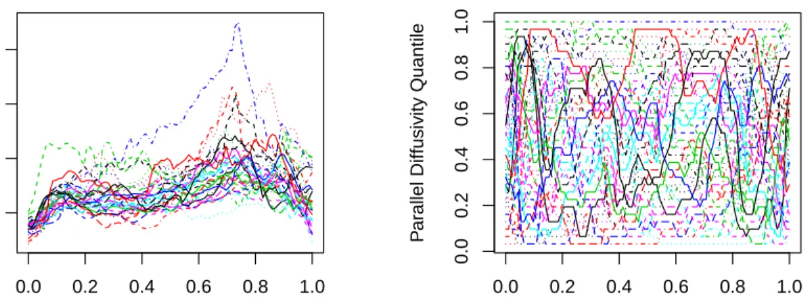
2.4 Application to Diffusion Tensor Imaging Dataset . . . 33

2.4.1 Predicting PASAT Score . . . 36

2.4.2 Predicting MS status: Logistic Link . . . 38

3 Sparse Covariates 41 3.1 Recovering Sparsely Observed Functional Data . . . 45

3.2 A Mixed Model Formulation of FGAM . . . 47

3.3 An MCMC algorithm for fitting FGAM . . . 51

3.4 A Variational Bayes Approach . . . 55

3.4.1 Review of Variational Bayes . . . 55

3.4.2 Fitting FGAM Using Variational Bayes . . . 57

3.5 Simulation Study . . . 60

3.6 Analysis of Auction Data . . . 64

4 Tests for Linearity 69 4.1 Restricted Maximum Likelihood Estimation . . . 70

4.2 LRTs and RLRTs for Linear Mixed Models . . . 72

4.3 Review of Bayes Factors . . . 74

4.4 More Mixed Models for Penalized Splines . . . 75

4.4.1 A Simple First Approach . . . 76

4.4.2 (Low Rank) Penalized Spline ANOVA Models . . . 77

4.5 A Test for Linearity of FGAM . . . 81

4.5.1 A Test For No Effect In the Functional Linear Model . . . . 85

4.6.1 Choice of Priors For the Variance Components . . . 86

4.6.2 An Approach Using Type IV Beta Priors . . . 90

4.6.3 An Approach Using Inverse-Gamma Priors . . . 94

4.7 Testing FLM Versus FGAM: Simulation Study . . . 95

4.7.1 True Model as Convex Combination of FLM and FGAM . . 98

4.7.2 True Model as SSANOVA-like Mixed Model . . . 101

4.8 Analysis of Emissions Data . . . 105

4.8.1 FLM Fit Assessment . . . 106

4.8.2 Out-of-Sample Prediction of Particulate Matter . . . 109

5 Discussion 112 5.1 Conclusions . . . 112

5.2 Open Questions and Future Work . . . 114

A Derivations For the Variational Bayes Algorithm 118 A.1 Derivation of Full Conditional Distributions . . . 118

A.2 Derivation of Optimal Proposal Densities . . . 120

A.3 Derivation of Log-Likelihood Lower Bound . . . 127

B Derivation Of Bayes Factors For Testing Linearity 133 B.1 For Arbitrary Number of Variance Components . . . 133

B.2 Alternative Expression For FGAM . . . 138

LIST OF TABLES

2.1 Simulation results for confidence band performance . . . 32

2.2 RMSE for prediction for DTI data . . . 38

3.1 Prediction accuracy results for auction data . . . 68

4.1 Rules for interpreting Bayes factors . . . 75

4.2 Description of tensor product construction for linearity tests . . . . 83

LIST OF FIGURES

2.1 Estimated surface for DTI data . . . 11

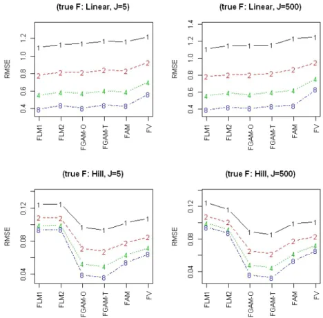
2.2 Simulation study of RMSE for prediction accuracy . . . 31

2.3 Observed parallel diffusivity measurements for DTI data . . . 35

2.4 Estimated surface contour plot for DTI data . . . 37

2.5 Bayesian confidence bands for estimated surface for DTI data . . . 39

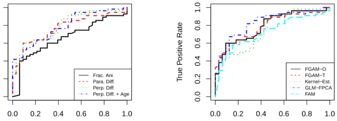
2.6 ROC curves for predicting disease status . . . 40

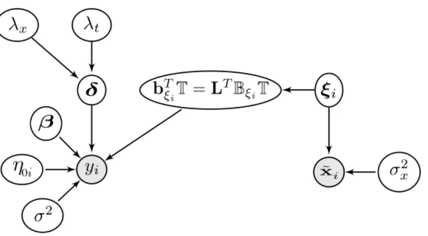
3.1 Directed acyclic graph for FGAM . . . 57

3.2 Sparse curves and true surfaces for simulation study . . . 61

3.3 Results from simulation study for sparse FGAM . . . 63

3.4 Prediction accuracy results of simulations for sparse FGAM . . . . 64

3.5 Estimated log-price ratio trajectories for auction data . . . 67

4.1 Results for Section 4.7.1 simulation study of testing methods . . . 100

4.2 Power of linearity tests for Section 4.7.2 simulation study . . . 103

4.3 Speed and acceleration trajectories for emissions study . . . 106

4.4 Diagnostics for FLM fit to emissions data . . . 107

4.5 Diagnostics for FGAMM fit to emissions data . . . 108

4.6 Contours of estimated surface for emissions data . . . 109

CHAPTER 1 INTRODUCTION

Firstly, wow! You are actually reading my thesis. Secondly, forgive me for my Canadian English; a bastardized version of proper, British English. It is much less bastardized than American English, but it’s still bastardized. Let’s get started.

1.1

A Brief Overview of Functional Data Analysis

The need for functional data analysis (FDA) tools has arisen as data sets have continued to balloon in size with advances in technology. In several fields, sampling can be done on such a fine grid that it makes sense to view each sample as being observed on a continuum and coming from a smooth function. The continuum is often, but not always, time; and the functions are often, but need not be, univariate. FDA methods have been successfully applied in a wide array of fields such as chemometrics, econometrics, and biomechanics. In this dissertation, we will demonstrate applications to brain imaging, online auctions, and automobile exhaust emissions.

First introduced in the seminal paper by Ramsay and Dalzell[89]_{, FDA is by} now a fairly mature, but still rapidly developing field. There currently are many applied and theoretical monographs available; including Ferraty[27]_{, Ferraty and} Romain[28], Ferraty and Vieu[29], Horváth and Kokoszka[44], Ramsay and Silver-man[90], Ramsay et al.[92], Shi and Choi[106], Zhang[136], and the standard introduc-tory reference Ramsay and Silverman[91]_{. There have been several special journal} editions on FDA and in R there are at least three software packages with a suite

of FDA methods available: fda (Ramsay et al.93_{), refund (Crainiceanu et al.}16_), and fda.usc(Febrero-Bande and Oviedo de la Fuente25_).

Paramount to any FDA, is that the underlying functions are smooth, i.e. that one or more of the functions’ derivatives exist. Smoothness of the functions is the key property that makes functional data methods advantageous over treating the data as discrete and using tools from multivariate statistics. Many of the methods of multivariate statistics have FDA counterparts. One of the most popular, which we will need in Chapter 3, is the extension of principal components analysis to functional data, called FPCA. (Hopefully, you can figure out that acronym all by yourself.) Typically, FPCA is one of the first methods considered in an FDA in order understand the underlying modes of variation present in the data. This is done by analyzing the eigenvalues and eigenfunctions of the functions’ covariance surface.

Another useful preliminary tool for FDA is registration, which enables the sampled functions to be compared more easily. This is achieved by aligning the observed curves to remove the effect of any uninformative horizontal (phase) shifts from function to function or aligning based on some shared characteristic, such as minima or maxima or points where the functions cross zero. One of the main uses of FDA is for the study of derivatives, differential equations, and dynamical systems. The FDA tool that will be the focus of this dissertation is that of using the sampled functions in a regression model in order to understand the relationship between the functions and some other variable(s) of interest. Methods are available for when either one or both of the response and predictor in the model are functions. We will concentrate on the case of predicting a scalar response when the predictors are functions.

We will introduce this topic in more detail after a short detour to multivariate data to discuss the key modelling tool used throughout the thesis, penalized splines.

1.2

Semiparametric Regression and Penalized Splines

Parametric models such as the multiple linear regression model, typically make very strong assumptions about the underlying data generation mechanism, assum-ing it depends only on a small number of parameters. Nonparametric models, on the other hand, make little to no assumptions about the underlying data generation and depend on an infinite number of parameters. As such, nonparametric models can be useful because they allow for capturing additional, more complicated struc-ture that parametric models cannot. Practically, we must index a nonparametric model by some large, but finite set of parameters. Semiparametric models are an attempt to provide the best of both worlds, consisting of models that have both parametric and nonparametric components.

Additive models are one of the most popular nonparametric tools for describing how a response variable depends on one or more covariates. Standard, early refer-ences are Buja et al.[8] and Hastie and Tibshirani[42]. Additive models allow the relationship between the response and a covariate to be modelled by an unspecified smooth function, but traditionally make the strong assumption that the covariates do not interact to avoid unacceptably large variance in estimation. In general, ad-ditive models offer increased flexibility and potentially lower estimation bias than linear models while having less variance in estimation and being less susceptible to the curse of dimensionality than models that make no additivity assumptions. The goal of this dissertation is to develop a model that provides greater flexibility

than the linear regression model for functional data (introduced shortly), while still being simple to estimate and interpret.

The unspecified regression functions mentioned above are represented using a linear combination of basis functions. B-splines will be our basis functions of choice throughout the dissertation because of their popularity and computational efficiency. A key idea is that we can take tensor products of marginal bases to represent functions of higher order in a simple manner.

Central to any nonparametric method is a tuning parameter (usually called a smoothing parameter) and penalty which control the complexity and smoothness of the estimated regression functions. The tuning parameter must be estimated from the data and adequate choice of tuning parameter is essential for the success of the method. Not smoothing enough results in overfitting, and estimates that have low bias but high variance that will provide poor predictions for new data. Smoothing too much results in models that fail to explain key features of the data.

By penalized splines, we mean that the regression function is represented using low rank spline bases subject to a quadratic roughness penalty. Great introductions to penalized splines can be found in Ruppert et al.[99] _{and Wood}[126]_{. In this work,} we will frequently make use of the P-splines of Eilers and Marx[20], which we will describe in detail later. The roughness penalty is often, but not always, the squared second derivative of the function. For P-splines, the penalties are differences (of a prespecified order) of adjacent B-splines. Once the type of basis and penalty are specified, the user must also specify/estimate the number of basis functions used to represent the function, the location of the knots (usually taken to just be equally spaced along the domain of the function), the order of the spline, the order of the penalty, and finally the value of the smoothing parameter that multiplies

the penalty. As mentioned, the smoothing parameter is the key component of the model controlling function shape (assuming one uses an adequate number of spline functions).

One concept extremely important for this dissertation, is that penalized spline models may be represented as mixed models, which allows for parameters to be estimated using techniques for those models. We will make use of a different mixed model representation in each of the three main chapters of this thesis. In Chapter 2, we only mention in passing that an alternative estimation procedure using mixed models is available, but in Chapters 3 and 4, the representations are fundamental to the methods used and we discuss them in detail. In Chapter 3, the mixed model representation used gives rise to a proper prior and results in a proper full conditional for the regression coefficients in a Bayesian version of our model. In Chapter 4, the third mixed model representation we consider allows us to explicitly show how the canonical model for functional regression is nested within our model providing a means for hypothesis tests regarding which model better fits the data.

1.3

The Scalar on Function Regression Landscape

This dissertation studies regression with a functional predictor and a scalar re-sponse. Suppose one observes data {(Xi(t), Yi) : t ∈ T } for i = 1, . . . , N, where

Xi is a real-valued, continuous, square-integrable, random curve on the compact interval T and Yi is a scalar. It is usually assumed that the predictor, X(·), is observed at a dense grid of points. The problem addressed here is estimation of

regres-sion model in functional data analysis is the functional linear model (Ramsay and Dalzell89_{), henceforth the FLM, given by}

E(Yi|Xi) =θ0+ Z

T β(t)Xi(t)dt, (1.1)

where β(·) is the functional coefficient with β(t) describing the effect on the re-sponse of the functional predictor at time t. We can see that for any fixed t, the effect ofX onY is linear. This model has been the subject of far too many papers to list. Ramsay and Silverman[91] _{provides a nice introduction and uses penalized} splines. Extensions to generalized responses are available (e.g., James46_{, Müller} and Stadtmüller75_).

The number of papers considering nonlinear models is considerably fewer. One model that has seen a fair amount of attention is the fully nonparametric kernel estimator of Ferraty and Vieu[29]. This model is more of a black box, sometimes useful for predictions, but not for providing any insights into how exactly the functional predictor affects the response. Several authors have considered addi-tive models that use linear functionals of the predictor curves as covariates, e.g.

E(Yi|Xi) =β0+f{hβ(t)Xi(t)i}=β0+f{ R

β(t)Xi(t)dt}, for unknownβ0, f(·), and

β(t). Two such examples are Müller and Yao[76]_{and James and Silverman}[47]_{. The} former approach regresses on a finite number of functional principal components scores and the latter approach searches for linear functionals using projection pur-suit. Both models rely strongly on the linear directions they estimate; for ease of in-terpretation, we desire a model that incorporates the functional predictors directly. A model that is additive in the principal component scores is not additive inX(t) itself, and vice versa. We have the same complaints about Ait-Saïdi et al.[1]_{, Chen} et al.[12]_{, Febrero-Bande et al.}[26]_{. Less general than our model is the functional} quadratic regression model of Yao and Müller[132]_{, which adds in the following term} to the FLM: R

T

R

com-petitors for the model we consider are Guillas and Lai[40]_{, which examines the case} when X is a bivariate function so that E(Yi|Xi) =β0+

R R

β(s, t)X(s, t)dsdt; and Li et al.[60]_{, which allows for interaction between a scalar and functional covariate} though a single index.

1.4

Contributions of This Dissertation

The model that we introduce and that will be the focus of the thesis is

g{E(Yi|Xi)}=θ0+ Z

T F{Xi(t), t}dt, (1.2)

where θ0 is the intercept, g is a called a link function, and F is an unspecified smooth function to be estimated. We call model (1.2) the functional generalized additive model (henceforth abbreviate as FGAM). As a special case, wheng(x) =x

and F(x, t) =β(t)Xi(t), we obtain the FLM (1.1).

Our model allows for greater flexibility in representing the response-predictor relationship, as it does not make the strong assumption of linearity between the functional predictor and the functional parameter. To overcome the curse of di-mensionality, we will perform smoothing in both thexandtcomponents ofF(·,·).

It will be shown that our model is the natural extension of generalized additive models (GAMs) to functional data.

The first core chapter of the dissertation shows how to estimate F(·,·) using penalized splines. We review tensor-product P-splines and show how they can be used to estimate FGAM using very fast and stable methods, and also discuss the implementation of FGAM in the popular statistics programming language R. Formulas for approximate confidence bands for the true regression surface are

given and we discuss how additional functional predictors can be incorporated in the model. We compare FGAM’s predictive performance with several other competing scalar-on-function regression models, including the FLM on simulated and real data sets and evaluate the coverage properties of the proposed confidence bands. We apply FGAM to a study in diffusion tensor imaging, where X(t) is a signal from the one-dimensional image at position,t, along a tract in the brain.

In order to extend FGAM to the common case where the functional predictors are sparsely observed and measured with error, we consider both Monte Carlo and variational Bayes (VB) methods for fitting the FGAM with sparsely observed co-variates and recovering the true functional predictors simultaneously. Variational Bayes (VB) refers to a specific variational approximation used for Bayesian infer-ence that relies on the assumption that a posterior density of interest factors into a product form over certain groups of model parameters. Though they are com-monly used in computer science, the application of variational approximations in statistics is relatively new; Ormerod and Wand[80]_{provides an overview. When the} amount of posterior dependence is small, there is little loss of accuracy and often very large improvements in computation time over MCMC methods. Applications of VB to regression problems with missing data can be found in Faes et al.[22] _and Goldsmith et al.[34]_{, the latter of which considered the FLM.}

Due to nonconjugacies in our model specification, we cannot use a vanilla Gibbs sampler or easily derive a simple VB algorithm. As such, the algorithms we de-velop are new and should be of independent interest. Our numerical experiments show the difficulties that can occur if one applies standard tools for recovering sparse curves and then attempts to run a functional regression as if the curves were fully observed, and demonstrates the superiority of our algorithms. In a real

data analysis, the methods are applied to forecasting closing price for items being auctioned on the online auction website eBay.

Finally, in the third part of the thesis we explore hypothesis tests for formally testing an FGAM fit for linearity. Through an alternative parametrization, we nest the FLM in the FGAM in a simple way that allows us to recast our testing problem as one of testing for zero variance components in a mixed model. We consider both restricted likelihood ratio tests and tests involving Bayes factors and g-priors. The use of these types of tests for checking for interactions in nonparametric models with bivariate functions has also not been considered before. The methods can also be used for testing for no effect in the functional linear model. The performance of the proposed tests is assessed on simulated data and in an application to measuring diesel truck emissions, where strong evidence of nonlinear effects in the data are found.

CHAPTER 2

DENSE COVARIATES

2.1

Preliminaries

2.1.1

Some Intuition for FGAM

To build intuition for the model, we start off immediately with an example. The application we consider in this chapter is diffusion tensor imaging (DTI), which we analyze in detail in Section 2.4. The dataset contains closely spaced evalua-tions of measures of neural functioning on multiple tracts in the brain for patients with multiple sclerosis and healthy controls. We will use these measurements as regressors and predict multiple health outcomes to gain a better understanding of how the disease is related to DTI signals. Our model is able to quantify the effect that the functional predictor has on the response at each position along the tract, something that a model such as the functional additive model of Müller and Yao[76] _{is unable to do, since it uses principal component scores and hence} loses information about tract location. Another potential application of FGAM is to study how a risk factor trajectory such as body mass index or systolic blood pressure is related to a health outcome such as developing hypertension (e.g., see the study in Li et al.59_{). Our FGAM can locate times of life when the risk factor} has its greatest effect; this is not possible if principal component scores are used in a GAM.

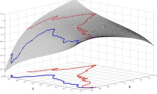
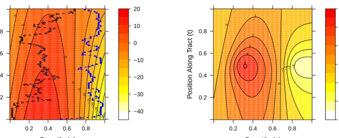
To see how our model can aid in uncovering the underlying structure of a func-tional regression problem consider Figure 2.1, which shows an estimated surface,

Figure 2.1: Estimated surface ˆF(x, t) and two predictor curves for the DTI dataset. The solid curve belongs to a control and the dashed curve belongs to an MS patient.

b

F(·,·), for one of the functional predictors in the DTI dataset when the response is disease status (= 1 if the subject has the disease). Overlaid on the surface are the observed functional predictor values for two subjects. The surface is non-linear in

x, so an FLM based on the predictors may be inadequate for this problem. We see that for the most part, the solid curve, belonging to a control subject, takes smaller values on the surface than the dashed curve, which belongs to a MS patient, does; thus, the subject with MS will have a higher fitted value and is more likely to be classified as having the disease. It will be shown for this dataset that the added generality of our approach leads to improved predictive accuracy over the FLM.

Additional insight can be gained by considering multivariate regression us-ing the raw, discrete data. The FLM can be thought of as multiple linear re-gression with an infinite number of predictors, as we now explain. Let tij = tj for 1, . . . , J denote the observation times for the curves Xi(·); then the usual

multiple linear regression model E(Yi|Xi(t1), . . . , Xi(tJ)) = β0 +PJi=1βjXi(tj) =

β0+J−1PJi=1β

0

jXi(tj) can be viewed as a Riemann sum approximation that con-verges to (1.1) as J → ∞.

Now consider an additive model of the form E{Yi|Xi(t1), . . . , Xi(tJ)} = θ0 + PJ

j=1fj{Xi(tj)}, where the fj’s are unspecified smooth functions. The basic idea is to rewrite the model asE{Yi|Xi(t1), . . . , Xi(tJ)}=θ0+J−1PJj=1F{Xi(tj), tj}, and then let J → ∞ and add a link function. The model obtained is our model (1.2). Hence, we believe are model to be the natural extension of additive models to functional data.

2.1.2

Parametrization of the Regression Surface

In this section, we introduce our representation for F(·,·). It is assumed that T = [0,1] and that X(·) takes values in a bounded interval which, without loss of generality, can be taken as [0,1]. The latter assumption is guaranteed by the proposed transformation of the functional predictors discussed in Section 2.1.4.

We will model F(·,·) using tensor products of B-splines. Splines are commonly used for estimation of functional linear models. For example, smoothing splines are used by Crambes et al.[18] and Yuan and Cai[133] and penalized splines are considered by Cardot et al.[10] _{and Goldsmith et al.}[32]_{. These papers impose} smoothness using a penalty on the integrated, squared second derivative of the coefficient function. Instead, we use the popular P-splines of Eilers and Marx[20]_. P-splines use low rank B-splines bases with equally-spaced knots and a simple difference penalty on adjacent coefficients to control smoothness.

P-splines. Namely, our design matrix is obtained from integrating products of B-splines evaluated at functional covariates. P-B-splines offer many computational advantages. Fast and flexible software is available for estimating our model in the

Rpackage refund (Crainiceanu et al.16_{) which makes use of smoothing parameter} selection algorithms available in mgcv (Wood127). Additional scalar or functional predictors can be incorporated in a simple way and will not require backfitting. Both types of predictors can be included in either a linear or an additive fashion. Though we use P-splines, our estimation procedure can incorporate other bases and penalties for some or all of the covariates. It will be shown that the fitted values for the FGAM are linear in the tensor product B-spline coefficients so we actually have a penalized generalized linear model (GLM). We use

A bivariate spline model is used for F(·,·) so that

F(x, t) = Kx X j=1 Kt X k=1 θj,kBjX(x)B T k(t) (2.1) where {BX

j (x) : j = 1, . . . , Kx} and {BkT(x) : k = 1, . . . , Kt} are spline bases on [0,1]. We will use B-spline bases. It follows from combining (1.2) and (2.1), that we obtain the GLM g{E(Yi|Xi)}=θ0+ Z T F{Xi(t), t}dt =θ0+ Kx X j=1 Kt X k=1 θj,kZj,k(i), (2.2) where Zj,k(i) = R

T BjX{Xi(t)}BkT(t)dt. Each Zj,k(i) can be approximated by, say, Simpson’s rule. Associated with each marginal basis are parameters, dx and dt, for the xand t bases, respectively, which specify the degree of differencing for the penalties for each axis. The penalties will be discussed in detail in Section 2.2.

2.1.3

Identifiability Constraints

Notice that for F∗(x, t) = F(x, t) + g(t), where R

T g(t)dt = 0 we have

R

T F∗(x, t)dt =

R

T F∗(x, t)dtand thus we must impose constraints to ensure

identi-fiability. If no constraints were used, the functiong(t) would be chosen to maximize the penalized log-likelihood given in Section 3.2 andg(t) would be regularized by the difference penalties we use. The penalties alone are not enough to ensure iden-tifiability, however. One possibility is to simply use a ridge penalty as in Marx and Eilers[67]_{. For our difference penalties, functions of t in the null space of the} penalty are polynomials of degreedt−1. Thereforedt−1 constraints are necessary for identifiability.

The constraint explicitly used by the fitting procedure isPN_i=1R

T F(Xi(t), t)dt = 0. Any additional constraint necessary to ensure identifiability are determined by checking for numerical rank deficiency during fitting. The details are explained in the next section.

For fixed smoothing parameters, different identifiability constraints yield the same predictions and the same estimated ˆF(·,·) up to a constant, though different estimates for the variance of the estimated surface (and therefore different confi-dence bands) will be obtained. The GCV score is also invariant to the constraints used. It is possible to switch to an alternative set of constraints after fitting our model using a pivoted QR decomposition along the lines of Wood et al.[129]_.

2.1.4

Transformation of the Predictors

Depending on the number of B-splines used for each axis, there could be a partic-ular tensor product of B-splines that has no observed data on its support. This would lead to Zj,k(i) = 0 for all i for some j, k pair, resulting in the design ma-trix containing a column of zeros. One remedy for this is to transform X(t) by

Gt(x) :=P{X(t)< x} for each value of t. Our model becomes

g{E(Yi|Xi)}=θ0+ Z T F[Gt{Xi(t)}, t]dt=θ0+ Kx X j=1 Kt X k=1 θj,k Z T B G j [Gt{Xi(t)}]BkT(t)dt, (2.3) where BG(·) is a new B-spline basis with support on [0,1]. Loosely, the data are being "stretched out" to fill the entire space that the grid of B-splines will cover. For any t on the grid where observations are taken, the transformed points will lie uniformly between [0,1]. Though the estimation procedure is the same in both cases, clearly, F(·,·) in (2.3) will have a different estimate from F(·,·) in (1.2). We estimate Gt(·) using the empirical cdf Gb_t(x) = n−1

n X i=1

I{Xi(t) < x}, where

I{A} = 1 if condition A is true and I{A} = 0 otherwise. Once the Zj,k(i)’s have been estimated, the fitting procedure is analogous to the case when the cdf transformation is not used. Another advantage of using this approach is that it does not require any assumptions about the range of the predictors. Besides the computational advantages, this transformation retains the benefit of ease of interpretation. In fact, F(p, t) is the effect of X(t) being at its pth quantile.

Another potentially useful transformation we do not pursue in this paper is ˆ

Ht(x) = n−1Pni=1Φ

h_x−Xi(t) ht

i

,where Φ(·) denotes the standard normal cdf andhtis a user chosen bandwith that can depend ont. The advantage of this transformation over the empirical cdf transformation is that future observations falling below [above] the minimum [maximum] value of the training data at a particular t are

not all assigned the value zero [one].

Due to the penalization used later when fitting the FGAM, parameter estimates can still be obtained when the design matrix has a column of zeros. However, we expect our transformation will improve both the numerical and statistical stability of our estimates. Note also that if there exists any pointwise transformation,Ht(·), such that g{E(Yi|Xi)} =RT β(t)Ht{Xi(t)}dt, then the FGAM will still hold; and similarly, for any model of the form (2.3) for a general transformation Gt(·). The FLM will hold only if Xi(t) is transformed byHt, but Ht is generally not known. Thus, the FGAM is invariant to transformations of the predictor, unlike the FLM.

2.2

Estimation

In this section, we present the estimation procedure for F(·,·). First, we review P-spline type penalties and discuss penalized GLMs and the selection of smoothing parameters. We then describe the estimated surface and discuss construction of pointwise confidence bands for these estimates. We conclude the section by showing how to include additional functional and non-functional predictors in the model.

2.2.1

Roughness Penalties

Smoothing can be achieved by using row and column penalties as in Marx and Eilers[67]_{. The row penalty is λ}

1PKxj=dx+1(∆ dx

j θj,k)2, where ∆dxj θj,k is the

dxth difference of the sequence θj−dx,k, . . . , θj,k (k held fixed). The column penalty isλ2PKtk=dt+1(∆

dt

kθj,k)2,where ∆dtkθj,k is thedtth difference of the sequence

discussed in the next section.

Proceeding similarly to Marx and Eilers[68]_{, we first place the Z}

j,k(i)’s in a matrix as follows. Let Zi = vec{Z(i)} be the KxKt-vector obtained by stacking the columns of _Z(i) = [Zj,k(i)] k=1,...,Kt j=1,...,Kx, and let Z = [Z1 Z2· · ·ZN] T . The penalty matrix is given by P=λ1PT1P1+λ2PT2P2, (2.4) with _P1 = Dx ⊗IKt, P2 = IKx ⊗Dt where Ip is the p×p identity matrix, ⊗ is the Kronecker product, and _Dx and Dt are matrix representations of the row and column difference penalties with dimension (Kx −dx)×Kx and (Kt−dt)×Kt, respectively. The parameter, d, denotes the prespecified degree of differencing. Note that additional penalties such as an overall ridge penalty could also be incor-porated.

To incorporate the intercept, a leading column of ones must be added to_Zand a leading column of zeros must be added to _P1 and P2. Throughout the rest of the paper, this has been done unless otherwise indicated. When we don’t wish to consider the intercept, _M[−i,−j] will denote the matrix M with itsith row and jth column removed and v[−i] will denote the vectorv excluding its ith entry.

2.2.2

Penalized GLMs and Smoothing Parameter Selection

Let the response vector,Y, be from an exponential family with density having the form fY(y;ζ, φ) = QNi=1exp [{yiζi−b(ζi)}/a(φ) +c(yi, φ)], where ζ is the canon-ical parameter vector with components satisfying ζi = (b0)−1(µi) and φ is the dispersion parameter. Parameterizing E(Y|_X) as a standard GLM with known link function, g(·), let η := _Zθ and µ := E(Y|_X), so that η = g(µ). It is

easily seen that the constraint, PN_i=1R

T F{Xi(t), t}dt = 0, is enforced by requir-ing 1T

Z[,−1]θ = 0. Formally, this is done by obtaining the QR decomposition of (1T_Z[,−1])T = [Q1 Q2]     r1 0KxKt−1    

, where _Q2 has dimension KxKt ×(KxKt −1). The constrained optimization problem is then replaced by an unconstrained opti-mization (outlined below) overθq,whereθq is such thatθ =Q2θq. For notational simplicity, for any matrix_M, define _Mf =_MQ2.

The penalized log-likelihood to be maximized is

l(θq;λ1, λ2) = N X i=1

log{fY(yi;ζi, φ)} −λ1||_Pe₁θ_q||2−λ₂||_Pe₂θ_q||2. (2.5) The coefficients are estimated using penalized iteratively re-weighted least squares (P-IRLS). Specifically, at the (m+ 1)th iteration we take

b θq,m+1 = e ZT_Wc_mZe +λ_1PeT 1Pe1+λ2_PeT 2Pe2 −1 e ZT_Wc_mu_bm, (2.6) whereubm is the current estimate of the adjusted dependent variable vector,u, and c

Wm is the current estimate of the diagonal weight matrix, W. The components of u are given by ui = ηi + (yi −µi)g0(µi). The ith diagonal element of W is

wii = 1/{V(µi)[g0(µi)]2}, with V(µi) = b00(ζi). To initialize the algorithm, use

µ₀ =Y and η₀ =g(Y), adjusting yi if necessary to avoidηi =∞.

To efficiently construct (2.6) and to detect rank deficiency, the following pro-cedure is used. First, use the QR-decomposition to form _W1/2_e

Z = QR where Q

is orthogonal, _R is upper triangular, and _W1/2 _{= diag(w}1/2

11 , . . . , w 1/2

N N). Next, use the Choleski decomposition to obtain _QT

2PQ2 = LTL. Pivoting should be used here because _P is positive semi-definite instead of positive definite. Now, from a singular value decomposition form [_RT

LT]T = UDVT, where U and V are

or-thogonal and_D is a diagonal matrix containing the singular values. At this point, we ensure identifiability by removing the columns and rows of _D and the columns

of _U and _V corresponding to singular values that are less than the square root of the machine precision times the largest singular value (Wood126_{, p. 183). It} then follows that (2.6) can be obtained from θb_q,m+1 =_VD−1_UT

1QTW1/2ubm,where

U1 is the sub-matrix of U satisfying R = U1DVT. At the final iteration, say M, our solution for θ is given by θb =_Q2θb_q,M and it can be shown that this satisfies 1T

Z[,−1]θb = 0 as required (Wood126, Sec. 1.8.1).

Generalized cross validation (GCV) can be used to choose the smoothing pa-rameters; see Wood[124]_{, Sec 4.5.4 for justification of its use for non-identity link} GAMs. The GCV score for λ1 and λ2 is given by

GCV(λ1, λ2) =

nD(Y;µb :λ1, λ2)

{n−γtr(_H)}2 , (2.7) where _H is known as the influence matrix and is related to the fitted values by

b

µ := g−1(_Zθb_M) = g−1(_Hu_M) and D(Y; b

µ : λ1, λ2) denotes the model deviance. The model deviance is defined to be twice the difference between the log-likelihoods of the saturated model, which has one parameter for each observation, and the given model. Formulas for the deviance for some common GLMs are given in McCullagh and Nelder[69]_{, Sec. 2.3; for example, for an identity link GLM,D(Y;}

b

µ:

λ1, λ2) = ||Y−HY||2. The constantγ ≥1 is usually chosen to take values between 1.2 and 1.4 to combat the tendency of GCV to undersmooth. For additional safeguards against undersmoothing, lower bounds could also be placed on the smoothing parameters.

A choice must be made on the order in which the P-IRLS and the smoothing pa-rameter selection iterations are performed. For what is termed outer iteration, for each pair of smoothing parameters considered, a GAM is estimated using P-IRLS until convergence. The other possibility, known as performance iteration, is to op-timize the smoothing parameters at each iteration of the P-IRLS algorithm. The

latter approach can be faster than outer iteration; however, it is more susceptible to convergence problems in the presence of multicollinearity (Wood126_{, Ch. 4).}

Our model can conveniently be fit in R using the mgcv package (Wood124_,128_). The details of how this is done are discussed in Section 2.2.6. We use outer iteration and Newton’s method for minimizing the GCV score, the package defaults. Using this package also allows for many possible extensions (e.g. mixed effects terms, formal model selection, alternative estimation procedures, etc.) beyond the scope of the current paper. Our code is implemented in the R package refund.

2.2.3

Estimated Surface

For a given θb, we can evaluate the estimated surface at any grid of points in its domain. Let X be an arbitrary column vector of length n1 taking values in the range of X(·) and T be the observation times or any vector of length n2 taking values in [0,1]. We let Fb denote the estimated surface evaluated on the mesh defined by X and T. To obtain Fb, let _Bx be the n₁n₂×K_x matrix of x-axis B-splines evaluated at X⊗1n2, i.e., Bx =

h BX₁ (X⊗1n2)· · ·B X Kx(X⊗1n2) i , where 1_n denotes a column vector of length n. Similarly, define _Bt as the n1n2 ×Kt matrix of B-splines evaluated at 1n1 ⊗T. Next, define then1n2×KxKt matrix

B= (Bx⊗1TKt)(1 T

Kx ⊗Bx), (2.8)

wheredenotes element-wise matrix multiplication. The estimated surface is then given by Fb =_Bθb_[−1].

2.2.4

Standard-Error Bands

For a response from any exponential family distribution, one simple way to con-struct approximate, pointwise confidence bands for Fb(x, t) conditional on the es-timated smoothing parameters is to use a sandwich estimator in the same manner as Hastie and Tibshirani[42]_{, Section 6.8.2 and Marx and Eilers}[67]_{. However, we} found through our simulation studies that these intervals do not have adequate coverage for our model, a result also noticed for univariate GAMs in Wood[125]_. This is because these intervals assume θb is unbiased, which will not be the case when θ6=0, due to the penalization involved in the estimation.

To overcome the bias in the parameter estimation, we use the Bayesian ap-proach of Wahba[117]_{. Using the improper priorπ(θ)∝exp−θ}T

Pθ/2 , it can be shown that θ|_ZT Wu, λ1, λ2 ∼N [_ZT_WZ+_P]−1_ZT_Wu,[_ZT_WZ+_P]−1φ,

see e.g. Wood[126]_{, Sec. 4.8. To estimate}

W, we use the estimated weight

ma-trix at the final P-IRLS iteration, _Wc_M. If it is necessary to estimate the dis-persion parameter, φ, we use φb = Pn

i=1V(ˆµi)−1(yi − µˆi)2/[N − tr(H)].

Let-ting _V bθ

= (_ZT_c

WMZ +P)−1φb and recalling that the estimated surface is given by Fb = Bθb_[−1], where _B is defined in (2.8), the variance of Fb is given by varhFb

i

= _BV

bθ[−1,−1]B

T_{. Taking Fb ±2}n_diagvarh_Fbio1/2 _{gives approximate 95%} empirical Bayesian confidence bands for F.

These Bayesian intervals have a nice frequentist property "across the function": in repeated random experiments with the same F, the observed coverage proba-bilities averaged over the observation points will tend to be close to the nominal coverage level. This property was borne out in several papers including Wahba[117]

and Nychka[79] _{for the case of smoothing splines and Wood}[125] _{for thin-plate} re-gression splines. Theoretical explanations for the property for generalized additive models were recently provided in Marra and Wood[65]_{. It will be examined for the} FGAM through a simulation study in Section 2.3.2.

Depending on the application, a particular linear combination of the elements of b

Fmay be of interest. If we letcbe a vector of the same length asFb, then we can also construct confidence bands of the formcT

b

F±2ncT _varh b

Fico1/2. For example, this could be used to determine approximately whether two observed curves have significantly different effects on the response at a particular value oft. Under a null hypothesis ofH0 :θ=0, θb is unbiased and we can use the sandwich estimator for the variance, _Vf =V

bθZ T_c

WMZV b

θ/φˆ, to conduct approximate hypothesis tests for

subsets ofθ. For example, we can construct surfaces of approximate t-statistics by scaling the estimated surface values by the reciprocal of their standard error (the diagonal elements of _Vf).

For any pointwise transformation, Ht(·), of the predictor used (including

Ht(x) = x), it is of interest to test whether ∂2/∂h2F(h, t) = 0 for all h and t, since this implies F{Ht(x), t} = β(t)Ht(x) for some function β(·). Since deriva-tives of B-splines are simple to compute, an estimate of the second derivative of the surface and the Bayesian confidence intervals for the second derivative are easily obtained by replacing _Bx in (2.8) with evaluations of the second derivatives of the

x-axis B-splines evaluated at the same points used for _Bx. While we cannot use our confidence bands for global inferences of this type, they do provide a rough heuristic for the desired test. We consider more formal tests of this hypothesis in Chapter 4. Marra and Wood[65] _{provides some evidence that coverage can be} im-proved slightly by including the intercept when calculating the proposed intervals

(which slightly changes the interpretation of the intervals as well). In our numer-ical studies, which we will discuss in detail shortly, we found that for FGAM the Bayesian confidence bands that did not include the intercept provided adequate coverage.

2.2.5

Multiple Predictors

Because of the modularity of penalized splines (Ruppert et al.99_{), including} mul-tiple functional predictors as well as scalar predictors in the model is straight-forward. Each additional functional predictor requires that two more smoothing parameters be selected. We will outline the procedure for the case of two func-tional covariates [say X1(·), X2(·)] and one scalar covariate (say W). The model isg{E(Yi|Xi,1, Xi,2, Wi)}=θ0+

R

T1F1{Xi,1(t), t}dt+

R

T2F2{Xi,2(t), t}dt+F3(Wi),

and both X1(·) and X2(·) can be transformed by their empirical cdfs. Further extensions are similar. As before, we use B-spline bases for both axes for both functional predictors and now also for W. One must also choose degrees of dif-ferencing to be used for each penalty. Let _Z(1) _and

Z(2) denoted the matrices of

integrated tensor product B-splines for X1 and X2, respectively. Similarly, define

P(1) and P(2) [see (2.4)]. Let B(W) be the matrix of W B-splines evaluated at the

observed values of W and let θ(W) be the corresponding vector of B-spline coeffi-cients forW. The penalty matrix for the smooth ofW is given by_P(W) _=λ

wDTwDw, where_Dw is the differencing matrix forW and λw is its smoothing parameter. For identifiability, add the constraint 1T

B(W)θ(W) = 0 (the usual constraint for each

functional component in a standard additive model). We place the same constraint on both functional predictors as in the previous section. Thus, we have three total

constraints. Construct

Z=

h

1 _B(W) _Z(1) _Z(2)i, _P= diag(0,_P(W),_P(1),_P(2)), and θ = (1,θ(W),θ(1),θ(2))T.

To accommodate a linear effect of the covariate W, replace _B(W) _in

Z with the

observed values ofW and replace _P(W) with zero in the above formula for _P. Note that it is also possible to have a linear effect for some functional predictors and additive effects for others; e.g. a model of the formg{E(Yi|Xi)}=θ0+f(Wi)+ R

T1β(t)X1i(t)dt +

R

T2F{X2i(t), t}dt. Using the roughness penalty approach for

estimating FLMs mentioned in Section 2.3.1, this can be implemented by making straightforward changes to_Z(1) _and

P(1) (see Ramsay and Silverman91, Ch. 15 for

details).

2.2.6

Fitting FGAM in

R

Let _X denote an N ×J matrix of the observed measurements of the functional predictor, whereN is the number of sampled curves and J is the number of mea-surements for each curve. Let _T denote the N ×J matrix of observation times for the predictor curves. Let_L denote theN ×J matrix of quadrature weights to use in our numerical integration of the surface F(x, t) and let y be the N-vector of observed response values. The simplest FGAM (using all the function defaults) and without an intercept is specified inrefund (Crainiceanu et al.16_{) by}

fgam(y~af(X,xind=T)-1).

The interface is meant to conveniently extend the functions lm and glmin baseR. As in those functions, the-1is included so that no intercept is fit; this is done here

to simplify the notation. The function af in the model formula is used to specify that the predictor X be fit in the FGAM form (1.2). See the documentation of either function for how to specify the spline bases used, how smoothing parameters are estimated, what penalties are used, etc. A functional predictor can also be fit as an FLM by using the functionlfin the formula specification. Also available are functions vis.fgam for visualizing FGAM fits and predict.fgam for predictions using an FGAM fit returned by a called to fgam.

The fgam function acts as a convenience wrapper for the gam, gamm, or bam

functions in package mgcv (Wood126_{). To understand what is being done by that} package, an equivalent call (with slightly different defaults) to fit the above FGAM inmgcv is

gam(y~te(X,T,by=L)-1),

where te specifies a tensor product smooth. The variables in the by argument to te are treated as the covariates in a varying coefficient model. To make this association more explicit, a generalized varying coefficient model has the form (e.g., see Wood126_{, p. 169).}

g(µi) = θ0+f1(xi1)xi2+f2(xi3, xi4)xi5+f3(xi6)xi7+. . . As a special case, consider

g(µi) =θ0+f(xi1, xi2)xi3+f(xi1, xi2)xi4+. . .+f(xi1, xi2)xi,J+2,

so each covariate, xi3, xi4, . . . , xi,J+2 has the same bivariate varying coefficient. Now suppose we have xi1 ≡ Xi(tj), xi2 ≡ tij ≡ tj , xip ≡ lij ≡ lj;p = j + 2;j = 1, . . . , Jwhere thelj’s are quadrature weights. Note thatmgcvtreats both variables

t and l as if they depend on i= 1, . . . , N though they do not for the FGAM. We now arrive at g(µi) =θ0+ J X j=1 f(xi1, xi2)xi,j+2 =θ0+ J X j=1 f{Xi(tj), tj}lj ≈θ0+ Z T f{Xi(t), t}dt,

somgcv is fitting the model

E(Yi|Xi) = J X j=1 F(xij, tij)lij = J X j=1 Kx X k=1 Kt X m=1 θkmBkX(xij)BmT(tij)lij, where as in the paper,BX

k (·) denotes the kth B-spline for thex-axis and Kx is the dimension of the basis for X (with equivalent definitions for the t-axis).

The matrix _BT which consists of J ×Kx blocks of sizeN ×Kt each is formed in mgcv. The (i, j) entry in the (m, n) block of _BT is given by BnX(xim)BjT(tim). The design matrix used for the smooth is then the N J×KxKt matrix

D= diag[vec(L)]BT

The package enforces one constraint at this point because the row sums of the

by variable matrix are constant (_L1 =0). The constraint is 1T

Dθ = 0. How to

implement this constraint during fitting and every other detail of the estimation procedure used by mgcv has already been discussed in this chapter.

The default smoothing method for a tensor product smooth in mgcv is cubic regression splines, so thebs argument tote must be specified as’ps’for P-splines to be used. The m argument to mgcv specifies both the order of the spline and the order of the penalty. For P-splines, m can be specified as a list with length equal to the number of marginal bases. The argumentk is a vector specifying the dimension of each marginal basis.

As an example, say we have an N-vector of responses y, the N ×J matrix of observed functional predictors _X with observation times occurring at equally

spaced points in [0,1], and that wish to use the midpoint rule aka rectangle method for approximating the integral. If we wish to use 10 cubic basis functions for the x-axis, 15 4th order basis functions for the t-axis, a second order difference penalty for the x-axis and a third order difference penalty for the t-axis, then the code to fit the FGAM with intercept is as follows

T=matrix( seq(0,1,l=J) ,N,J) L=matrix(1/J,N,J)

fit=gam( y~te(X,T,by=’L’,bs=’ps’,k=c(10,15),m=list(c(2,2),c(4,3))) )

Note that in the documentation for P-spline smooths in mgcv (see?p.spline), it is noted that a smooth term of the form

s(x,bs="ps",m=c(2,3))

”specifies a 2nd order P-spline basis (cubic spline), with a third order difference penalty...” Though it is not standard for a cubic spline to be called 2nd order, this does seem to be what is implemented withinmgcvand so we follow along with this specification.

Additional functional predictors are added by including additional te terms. Responses from other exponential family distributions are handled in the exact same way as theglm function in R.

2.3

Simulation Experiment

In this section, we perform simulations to assess the empirical performance of our FGAM. We first assess the ability of our FGAM to predict out-of-sample data

in the Gaussian response case and compare its performance with several other functional regression models. Next, we examine the coverage properties of the empirical Bayesian confidence bands proposed in Section 2.2.4.

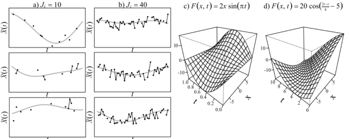
To generate the data, we created 1000 replicate data sets each consisting of

N curves sampled at 200 equally-spaced points in [0,1] as follows: Let Xi(t) = PJ

j=1γj[Z1ijφ1j(t)+Z2ijφ2j(t)] whereZhij ∼N(0,1),φ1j(t) = √

2 cos(πjt),φ1j(t) = √

2 sin(πjt), and γj = 2_j; h = 1,2; i = 1, . . . , N; j = 1, . . . , J. We consider two values for J, J = 5 and J = 500, the former resulting in much smoother predictor trajectories. We examine two cases for the true surface, F(x, t), one where the FLM holds, F(X(t), t) = β(t)X(t) and the other where it does not. For the linear true model, F(x, t) = xt. For the nonlinear true model, we use

F(x, t) =−.5 + exph−(x 5)

2₋₍t−.5 .3 )

2i_{, which looks like a hill or bivariate normal} density.

The error variance changes with each sample so that the empir-ical signal to noise ratio (SNR) defined by SNR=s

2 ˆ y σ2, where s2_yˆ = 1 N−1 N X i=1 h_R T F(Xi(t), t)dt−N−1PNi=1 R T F(Xi(t), t)dt i2

remains constant. We con-sider the values SNR= 1,2,4,8 in our simulations.

2.3.1

Out-of-Sample Predictive Performance

We fit FGAM and compare its out-of-sample predictive accuracy with three other popular functional regression models, the FLM, the kernel estimator of Ferraty and Vieu[29]_{, and the functional additive model (FAM) of Müller and Yao}[76]_{. The} coding used in our analyses was done in R (R Core Team88_{). The fda package} (Ramsay et al.93) implements the standard tools of functional data analysis in R.

As an initial step in fitting our model, the FLMs and the FAM, we use this package to smooth the data using B-spline basis functions and a roughness penalty with smoothing parameter chosen by GCV.

There are two main approaches for estimating the coefficient function β(·) for a FLM. The first uses smoothing or penalized splines and the second uses a func-tional principal component analysis (fPCA). We refer to these as FLM1 and FLM2, respectively. These models can be fit in Rusing the fda package, more specifically, the functions fRegress for FLM1 and pca.fd for FLM2. See Ramsay et al.[92]_, Chapter 9 for computational details. For FLM1, we choose the smoothing param-eter by minimizing GCV. For FLM2, we conduct a functional principal component analysis with a constant, light amount of smoothing and retain enough compo-nents for each simulation scenario to explain 90% of the total variability of the functional predictor. Once the scores are estimated, the final step to estimating FLM2 is fitting an unpenalized linear model in the scores.

To fit the FAM, we use the same number of principal component scores and the same estimation procedure as for FLM2. The difference comes in the next step, where a generalized additive model is fit using the scores as predictors. To estimate the GAM, we use the default settings in the mgcv package and 11 basis functions for each additive term.

The final model we fit is described in detail in Ferraty and Vieu[29]_{, Ch. 5. The} response is predicted by the nonlinear operator r(X) := E(Y|X). This operator is estimated by a functional extension of the Nadaraya-Watson kernel estimator:

b r(X) = PN i=1YiK{h−1d(X, Xi)} PN i=1K{h−1d(X, Xi)} , (2.9)

where K is an asymmetrical kernel with bandwidth h and d is a semimetric. Continuity or Lipschitz continuity of the regression operator in the semimetric