Nonparametric Estimation and Model Combination in a Bandit Problem with Covariates

(1)

Nonparametric Estimation and Model Combination in a

Bandit Problem with Covariates

A DISSERTATION

SUBMITTED TO THE FACULTY OF THE GRADUATE SCHOOL OF THE UNIVERSITY OF MINNESOTA

BY

Wei Qian

IN PARTIAL FULFILLMENT OF THE REQUIREMENTS FOR THE DEGREE OF

Doctor of Philosophy

Advisor: Dr. Yuhong Yang

(2)

c

(3)

Acknowledgements

I have received enormous support from a number of individuals over the past six years. I am very grateful that Professor Yuhong Yang has been my mentor, and guided me through several research projects including this dissertation research. His knowledge, generosity and patience have profoundly influenced me, and reshaped my life forever in many important aspects. The extremely rewarding endeavor with him in the past few years has ignited my ever-lasting interests and passion for statistics research and applications. What I have learned from him will certainly continue to be of great help for many years to come.

I would like to thank Professor Lan Wang for chairing my thesis committee, and being an excellent instructor for multiple fundamentally important statistics courses I took. I would also like to thank Professor Adam Rothman and Professor Bert Fristedt for spending their time serving as my committee members, reviewing my thesis work, and providing insightful suggestions on the research and career development. I am also grateful to Professor Hui Zou, Professor Dennis Cook and Professor Tiefeng Jiang for helping to broaden my research horizons and further my research interests in various directions.

I have also been the beneficiary of the very supporting environment in the School of Statistics at the University of Minnesota. In addition to all faculty and staff members in our school, I would like to thank my fellow classmates for helping me in every step of my academic development. I truly appreciate their friendship and help from the very first day of my study here.

Finally, I want to thank my parents and Shanshan for their love and support. The happiness and trust they give me is always my source of strength that keeps me moving forward.

(4)

Dedication

To my parents Jianping Qian and Minhe Wei for their unwavering support and encour-agement.

(5)

Abstract

Multi-armed bandit problem is an important optimization game that requires an exploration-exploitation tradeoff to achieve optimal total reward. Motivated from in-dustrial applications such as online advertising and clinical research, we consider a setting where the rewards of bandit machines are associated with covariates. Under a flexible problem setup, we focus on a sequential randomized allocation strategy, under which, the “plug-in” regression methods for the estimation of mean reward functions play an important role in the algorithm performance. In the first part of the disserta-tion, we study the kernel estimation based randomized allocation strategy, and establish asymptotic strong consistency and finite-time regret analysis.

In addition, although many nonparametric and parametric estimation methods in supervised learning may be applied to the randomized allocation strategy in a conve-nient “plug-in” fashion, guidance on how to choose among these estimation methods is generally unavailable. In the second part of the dissertation, we study a model com-bining allocation strategy for adaptive performance, and establish its asymptotic strong consistency. Simulations and a real data evaluation are conducted to illustrate the performance of the proposed combining strategy.

In the existing literature of nonparametric bandit problem with covariates, it is gen-erally assumed that the smoothness parameters of a H¨older condition for the reward functions are known. Also, the finite-time regret analysis in the first part of the disser-tation remains minimax sub-optimal. In the third part of the disserdisser-tation, we address these two issues by proposing a multi-stage randomized allocation strategy with arm elimination. In particular, when the smoothness parameter is unknown, we equip the algorithm with a smoothness parameter selector based on Lepski’s method, and show that the regret minimax rate is achieved up to a logarithmic factor.

(6)

List of Tables

3.1 (Case 1) Weights of bandwidth choices for Nadaraya-Watson regressions from the last repeat . . . 32 3.2 (Case 2) Weights for combining Nadaraya-Watson (NW) regression and

linear regression . . . 34 3.3 Comparing the estimated dimension reduction matrix ˆB₂∗_,Nfor the second

arm between SIR and CIS-SIR. . . 36 3.4 Normalized CTRs of various algorithms on the news article

recommenda-tion dataset. CTRs are normalized with respect to the random algorithm. 38

(9)

List of Figures

3.1 (Case 1) Combining Nadaraya-Watson regressions with different band-width choices. Left panel: averaged per-round regret. Right panel: aver-aged inferior sampling rate. . . 32 3.2 (Case 1) Averaged per-round regret from combining different methods.

Left panel: combiningK-nearest neighbor methods with different choices ofK. Right panel: combining different nonparametric methods. . . 33 3.3 Averaged per-round regret from combining different methods. Left panel:

(Case 2) combining Nadaraya-Watson regression and linear regression. Right panel: (the multivariate covariate case) comparing SIR and CIS-SIR. 34 3.4 Boxplots of normalized CTRs of various algorithms on the news

arti-cle recommendation dataset. Algorithms include (from left to right): LinUCB,-greedy, SIR-kernel (hn1), SIR-kernel (hn2), SIR-kernel (hn3),

model combining with SIR-kernel (hn3) and-greedy. CTRs are

normal-ized with respect to the random algorithm. . . 39

(10)

Chapter 1

Introduction

1.1 Multi-Armed Bandit Problem

Following the seminal work by Robbins (1954), multi-armed bandit problems have been studied in multiple fields. The general bandit problem involves the following optimiza-tion game: A gambler is given l gambling machines, and each machine has an “arm” the gambler can pull to receive the reward. The distribution of reward for each arm is unknown to the gambler. At each round of the game, the gambler is allowed to play one and only one of these arms. The goal is to maximize the total reward over a given time horizon. If we define the regret to be the reward difference between the optimal arm and the pulled arm, the equivalent goal of the bandit problem is to minimize the total regret. Under a standard setting, it is assumed that the reward of each arm has fixed mean and variance throughout the time horizon of the game. Some of the representative work for standard bandit problem includes Lai and Robbins (1985), Berry and Fristedt (1985), Gittins (1989) and Auer et al. (2002). Recent overviews of Cesa-Bianchi and Lugosi (2006) and Bubeck and Cesa-Bianchi (2012) include many of its extensions.

An algorithm for bandit problem usually involves a trade-off between “exploration” and “exploitation”. On the one hand, we want to pull the arm of each machine as many times as possible so as to explore the true reward distribution of each arm; on the other hand, we want to exploit the information obtained from the previous arm pullings and play the “best” arm and realize the gain. Clearly, exploration alone or exploitation alone cannot result in an optimal strategy: excessive pulling of all arms would give results no

(11)

better than a completely randomized strategy, while constantly pulling the “best” arm is certainly sub-optimal if the exploitation decision is made based on the wrong initial information about the reward distributions.

Next, we review some main algorithms for the standard multi-armed bandit problem. Suppose in a classic l-armed bandit problem, the rewards associated with the bandit machines have expected valuesµ1,· · · , µland varianceσ12,· · · , σl2. With a time horizon

N, let ˆµ1(n),· · ·,µˆl(n),n= 0,1,· · ·, N, be the empirical estimate (typically calculated

as the sample mean) ofµ1,· · ·, µl at timen. Define the expected cumulative regretRn

of an algorithm to be the difference between the expected reward by always pulling the best arm and the expected reward of this algorithm from time 0 to time n . We can consider the following algorithms.

Pure Greedy. Pure greedy is the simple-minded exploitation-only algorithm. Af-ter initial random exploration, the player always pulls the arm with the highest empirical estimate of the expected reward. Clearly, this strategy can suffer from the insufficient exploration at the initial stage.

Upper Confidence Bound (UCB). UCB algorithm is first introduced by Lai and Robbins (1985). At timen, the upper bound index for the expected reward functions are calculated, and the arm with the highest upper bound index is pulled. In this classical paper, they show that for some specific family of reward distributions, any suboptimal arm isatisfies

E[Ni(n)]≤ 1 Di +o(1) logn

where Ni(n) is the number of times arm iis pulled during the first n plays, and Di is

the Kullback-Leibler divergence between the reward density of arm i and the reward density of the optimal arm. They also show that this upper bound is asymptotically optimal. Auer et al. (2002) proposes several computationally simpler UCB algorithms, and show that they achieve logarithmic regret uniformly instead of only asymptotically. In addition, the upper confidence bound used in their algorithms have the form very similar to the upper confidence bound of a regular sample mean for i.i.d observations.

(12)

Exponential Weighting. Let pi(n) denote the probability of pulling arm i, 1 ≤

i ≤ l, at time n. For exponential weighting algorithms, pi(n+ 1) is updated based

on the action and observation at previous time points. The SoftMax strategy (Luce, 1959) is a simple version of exponential weighting, which pulls the armiat timenwith probability pi(n) = exp(ˆµi(n)/τ) Pl k=1exp(ˆµk(n)/τ) ,

where τ is a tuning parameter. A more complicated version called “exponential-weight algorithm for exploration and exploitation” (Exp3) is first introduced by Auer (2002). With the implicit assumption that an infinite sequence of time-dependent reward has been assigned to each bandit machine, Exp3 starts with the weights wi(1) = 1 for

i= 1,· · · , l, and updates the probability by pi(n) = (1−γ) wi(n) Pl k=1wj(n) +γ l, 1≤i≤l.

If arm i is pulled at time n and gives the corresponding reward yi(n), update the

weights by wi(n+ 1) = wi(n) exp(γyi(n)/pi(n)). Otherwise, update the weights by

wi(n+ 1) =wi(n). The tuning parameter γ ∈(0,1] can be chosen by the user.

-Greedy. Different from pure greedy strategy, -greedy implements an enforced randomization strategy, pulling the arm of the highest empirical estimate with probabil-ity 1−while pulling the rest of the arms with equal probability _l−₁. With a constant, it is clear that this strategy can be inefficient since exploration of the sub-optimal arms continues even after the optimal arm is apparent. A closely related variant, which is sometimes called -decreasing, overcomes such inefficiency by letting →0 asn→ ∞. By appropriately choosing a decreasing sequence of , Auer et al. (2002) shows that the expected regret has an optimal bound of O(logn). Extensive numerical study by Vermorel and Mohri (2005) also show that -decreasing strategy performs rather well compared with other sophisticated algorithms.

(13)

1.2 Bandit Problem with Covariates

Different variants of the bandit problem motivated by real applications have been stud-ied extensively very recently. One promising setting is to assume that the reward dis-tribution of each bandit arm is associated with some common external covariate. More specifically, for an l-armed bandit problem, the game player is given a d-dimensional external covariate x∈Rd _{at each round of the game, and the expected reward of each}

bandit arm given x can have a functional form fi(x), i = 1· · · , l. We call this

vari-ant multi-armed bandit problem with covariates, or MABC for its abbreviation. The consideration of external covariates is potentially important in applications such as per-sonalized medicine. For example, before deciding which treatment arm to be assigned to a patient, we can observe the patient prognostic factors such as age, blood pressure or genetic information, and then use such information for adaptive treatment assignment to improve the overall well-being of the patients.

The MABC problems have been studied under both parametric and nonparametric frameworks with various types of algorithms. The first work in a parametric framework appears in Woodroofe (1979) under a somewhat restrictive setting. With settings more flexible than that of Woodroofe (1979), a linear response bandit problem is recently studied under a minimax framework (Goldenshluger and Zeevi, 2009; Goldenshluger and Zeevi, 2013). Empirical studies are also reported for parametric UCB-type algorithms (e.g., Li et al., 2010). The regret analysis of a special linear setting are given in e.g., Auer (2002), Chu et al. (2011) and Agrawal and Goyal (2013), in which the linear parameters are assumed to be the same for all arms while the observed covariates can be different across different arms.

MABC problems with the nonparametric framework are first studied by Yang and Zhu (2002). Yang and Zhu (2002) show that with histogram or K-nearest neighbor estimation, the function estimation is uniformly strongly consistent, and consequently, the cumulative reward of their randomized allocation rule is asymptotically equivalent to the optimal cumulative reward. Their notion of reward strong consistency has been recently established for a Bayesian sampling method (May et al., 2012). Notably, under the H¨older smoothness condition and a margin condition, the recent work of Perchet and Rigollet (2013) establishes a regret upper bound by arm elimination algorithms with

(14)

the same order as the minimax lower bound of a two-armed MABC problem (Rigollet and Zeevi, 2010). A different stream of work represented by, e.g., Langford and Zhang (2008) and Dudik et al. (2011) imposes neither linear nor any smoothness assumption on the mean reward function; instead, they consider a class of (finitely many) policies, and the cumulative reward of the proposed algorithms is compared to the best of the policies.

Another important line of development in bandit problem literature (closely related to, but different from the setting of MABC) is to consider the arm space as opposed to the covariate space in MABC. It is assumed that there are infinitely many arms, and at each round of the game, the player has the freedom to play one arm chosen from the arm metric space. Like MABC, the setting with the arm space can be studied from both parametric (linear) framework and nonparametric framework. Examples of the para-metric framework include Dani et al. (2008), Rusmevichientong and Tsitsiklis (2010) and Abbasi-Yadkori et al. (2011). Notable examples of the nonparametric framework (also known as the continuum-armed bandit problem) under the local or global H¨older and Lipchitz smoothness conditions are Auer et al. (2007), Kleinberg et al. (2007) and Bubeck et al. (2011). Interestingly, Lu et al. (2010) and Slivkins (2011) consider both the arm space and the covariate space, and study the problem by imposing Lipschitz conditions on the joint space of arms and covariates.

Our work follows the nonparametric framework of MABC in Yang and Zhu (2002) and Rigollet and Zeevi (2010) with finitely many arms. As one motivation of our work, previous nonparametric approaches to MABC are limited to simple averages of clusters of observed rewards, which gives only discontinuous estimated functions, while It is known that kernel methods can generate continuous estimates and potentially improve estimation efficiency for smooth targets. The kernel regression analysis results under i.i.d. or weak dependence settings are well-established in, e.g., Devroye, 1978; H¨adle and Luckhaus, 1984; Hansen, 2008. One of our contributions is to show, under the MABC setting, that kernel methods enjoy estimation uniform strong consistency as well, which leads to strongly consistent allocation rules. In addition, with the help of the H¨older smoothness condition, we provide a finite-time regret analysis for the proposed randomized allocation strategy. Our result explicitly shows both the bias-variance tradeoff and the exploration-exploitation tradeoff, which reflects the underlying

(15)

nature of the proposed algorithm for the MABC problem. Moreover, with a model combining strategy along with the dimension reduction technique to be introduced later, the kernel method based allocation strategy can be quite flexible with potential practical use.

One natural and interesting issue in the randomized allocation strategy in MABC is how to choose the modeling methods among numerous nonparametric and paramet-ric estimation approaches. The motivation of such question shares the flavor of model aggregation/combining in statistical learning, which targets to achieve prediction per-formance almost as well as the best of the prediction candidates (see, e.g., Audibert, 2009 and references therein). In the bandit problem literature, model combining is also quite relevant to the adversary bandit problem (Auer et al., 2003). As a recent example, Maillard and Munos (2011) study the history-dependent adversary bandit to target the best among a pool of history class mapping strategies.

As an empirical solution to our attempt to choose the best estimation method for each arm in the randomized allocation strategy for MABC, we introduce a fully data-driven model combining technique motivated by the AFTER algorithm, which has shown success both theoretically (Yang, 2004) and empirically (e.g., Zou and Yang, 2004; Wei and Yang, 2012). We integrate a model combining step by AFTER for re-ward function estimation into the randomized allocation strategy for MABC. As another contribution, we present here new theoretical and numerical results on the proposed combining algorithm. In particular, the strong consistency of the model combining allocation strategy is established.

Since the H¨older smoothness condition is usually assumed for MABC from nonpara-metric perspective, the last question this dissertation attempts to address is whether we can achieve a guaranteed regret upper bound without the prior knowledge of the smoothness parameter. Our solution to such question is closely related to the adaptive nonparametric estimation technique pioneered by Lepski (1990). The “Lepski-type” method has recently been studied to establish the adaptive confidence bands for density estimation and regression problems in Gin´e and Nickl (2010), Hoffmann and Nickl (2011) and Bull, 2012. Their “self-similarity” condition is employed here to study the adap-tive performance of the proposed MABC algorithm. By imbedding the “Lepski-type” method and an arm-elimination subroutine (Even-Dar et al., 2006; Perchet and Rigollet,

(16)

2013) into the randomized allocation strategy, we show that the resulting cumulative regret adaptively achieves the minimax rate up to a logarithmic factor.

This dissertation is organized as follows. Chapter 2 introduces the problem setup for MABC and a randomized allocation strategy with model combination. In particu-lar, we focus on the kernel estimation method, and study the strong consistency and the finite-time regret analysis for the proposed algorithm. In Chapter 3, we study the asymptotic property of the model combining allocation strategy, and evaluate its empir-ical performance by simulations and a web-based news article recommendation dataset. In Chapter 4, we propose a randomized allocation strategy with arm elimination to show the adaptive performance when combined with the “Lepski-type” method.

(17)

Chapter 2

Kernel Estimation in a Bandit

Problem with Covariate

2.1 Problem Setup

Suppose a bandit problem has l (l ≥ 2) candidate arms to play. At each time point of the game, a d-dimensional covariate x is observed before we decide which arm to pull. Assume that the covariate x takes values in the hypercube [0,1]d. Also assume the (conditional) mean reward for arm igiven x, denoted byfi(x), is uniformly upper

bounded and unknown to game players. The observed reward is modeled as fi(x) +ε,

where εis a random error with mean 0.

Let{Xn, n≥1} be a sequence of independent covariates generated from an

under-lying probability distribution PX supported in [0,1]d. At each time n≥1, we need to

apply a sequential allocation rule η to decide which arm to pull based on Xn and the

previous observations. We denote the chosen arm by In and the observed reward of

pulling the arm In=i at timen by Yi,n, 1≤i≤l. As a result,YIn,n =fIn(Xn) +εn,

whereεn is the random error, and (Xn,εn) are independent of the earlier observations.

Different from Yang and Zhu (2002), we shall not assume that the error εn and the

covariateXnare independent. Consider the simple scenario of online advertising where

the response is binary (click: Y = 1; no click: Y = 0). Given an armi and covariate x∈[0,1], suppose the mean reward function satisfies e.g.,fi(x) =x. Then it is easy to

see that the distribution of the random error ε depends on x. In case of a continuous 8

(18)

response, it is also well-known that heteroscedastic errors commonly occur.

The errorsεn are often assumed to have a bounded support in bandit problem

liter-ature. We will see that such an assumption can be avoided to allow distributions with other types of tails. When dealing with a continuous response, this weaker requirement substantially enhance applicability of the results in real problems.

By the previous definitions, we know that at timen, an allocation strategy chooses the armInbased onXnand (Xj,Ij,YIj,j), 1≤j ≤n−1. To evaluate the performance

of the allocation strategy, leti∗(x) = argmax₁≤i≤lfi(x) andf∗(x) =fi∗₍_x₎(x). Without

the knowledge of random error εj, the optimal performance occurs when Ij =i∗(Xj),

and the corresponding optimal cumulative reward givenX1,· · ·, Xn can be represented

as Pn

j=1f∗(Xj). The cumulative mean reward of the applied allocation rule can be

represented as Pn

j=1fIn(Xj). Thus we can measure the performance of an allocation

rule η by the cumulative regret Rn(η) = n X j=1 f∗(Xj)−fIj(Xj) .

We say the allocation ruleη is strongly consistent ifRn(η) =o(n) with probability one.

Also, Rn(η) is commonly used for finite-time regret analysis. In addition, define the

per-round regret rn(η) by rn(η) = 1 n n X j=1 f∗(Xj)−fIj(Xj) .

To maintain the readability for the rest of this chapter, we useionly for bandit arms, j and nonly for time points,r and sonly for reward function estimation methods, and t and T only for the total number of times a specific arm is pulled.

2.2 Algorithm

In this section, we present the randomized allocation strategy. For convenience, a model combining procedure is imbedded into the algorithm, which will be discussed in Chapter 3. At each timen≥1, denote the set of past observations{(Xj, Ij, YIj,j) : 1≤j ≤n−1}

by Zn, and denote the arm i associated subset {(X_j, Ij, YIj,j) :Ij =i, 1 ≤j ≤n−1}

by Zn,i_{. For estimating the} _f

(19)

procedures (e.g., histogram, kernel estimation, etc.), and we denote the class of these candidate procedures by ∆ = {δ1,· · · , δm}. Let ˆfi,n,r denote the regression estimate

of procedure δr based on Zn,i, and let ˆfi,n denote the weighted average of ˆfi,n,r’s,

1 ≤ r ≤ m, by the model combining algorithm to be given. Let {π_n, n ≥ 1} be a decreasing sequence of positive numbers approaching 0, and assume that (l−1)πn<1

for all n≥1. The model combining allocation strategy includes the following steps. STEP 1. Initialize with forced arm selections. Give each arm a small number of

appli-cations. For example, we may pull each arm n0 times at the beginning by taking

I1= 1, I2= 2,· · ·Il=l,Il+1 = 1,· · · , I2l=l,· · ·, I(n0−1)l+1= 1,· · ·, In0l=l.

STEP 2. Initialize the weights and the error variance estimates. For n = n0l+ 1,

initialize the weights by

Wi,n,r=

1

m, 1≤i≤l,1≤r≤m, and initialize the error variance estimates by e.g.,

ˆ

vi,n,r= 1,ˆvi,n= 1, 1≤i≤l,1≤r ≤m.

STEP 3. Estimate the individual functionsfi for 1≤i≤l. Forn=n0l+ 1, based on

the current data Zn,i, obtain ˆfi,n,r using regression procedureδr, 1≤r ≤m.

STEP 4. Combine the regression estimates and obtain the weighted average estimates ˆ fi,n= m X r=1 Wi,n,rfˆi,n,r, 1≤i≤l.

STEP 5. Estimate the best arm, select and pull. For the covariate Xn, define ˆin =

argmax₁_≤i≤lfˆi,n(Xn) (If there is a tie, any tie-breaking rule may apply). Choose

an arm, with probability 1−(l−1)πn for arm ˆin (the currently most promising

choice) and with probability πn for each of the remaining arms. That is,

In=    ˆ_i_n_, _{with probability 1}₋_(l₋_1)π_n_, i, with probability πn, i6= ˆin,1≤i≤l.

(20)

STEP 6. Update the weights and the error variance estimates. For 1≤i≤l, ifi6=In,

let Wi,n+1,r =Wi,n,r, 1≤r≤m, ˆvi,n+1,r = ˆvi,n,r, 1≤r≤m, and ˆvi,n+1 = ˆvi,n. If

i=In, update the weights and the error variance estimates by

Wi,n+1,r = Wi,n,r ˆ v_i,n,r1/2 exp −( ˆfi,n,r(Xn)−Yi,n) 2 2ˆvi,n ! m X k=1 Wi,n,k ˆ v1_i,n,k/2

exp −( ˆfi,n,k(Xn)−Yi,n)

2 2ˆvi,n !, 1≤r ≤m, ˆ vi,n+1,r = n X k=n0l+1 (YIk,k−fˆIk,k,r(Xk)) 2_I(I k=i) n X k=n0l+1 I(Ik =i) , 1≤r≤m, and ˆ vi,n+1 = n X r=1 Wi,n+1,rvˆi,n+1,r,

where I(·) is the indicator function.

STEP 7. Repeat steps 3 - 6 for n=n0l+ 2, n0l+ 3,· · ·, and so on.

In the allocation strategy above, step 1 and step 2 initialize the game and pull each arm the same number of times. Step 3 and step 4 estimate the reward function for each arm using several regression methods, and combine the estimates by a weighted average scheme. Clearly, the importance of these regression methods are differentiated by their corresponding weights. Step 5 performs an enforced randomization algorithm, which gives preference to the arm with the highest reward estimate. Step 6 is the key to the model combining algorithm, which updates the weights for the recently played arm. Its weight updating formula implies that if the estimated reward from a regression method turns out to be far away from the observed reward, we penalize this method by decreasing its weight, while if the estimated reward turns out to be accurate, we reward this method by increasing its weight.

(21)

2.3 Kernel Regression Procedures

In this section, we consider the special case that kernel estimation is used as the only modeling method. The primary goals include: 1) establishing the uniform strong con-sistency of kernel estimation under the proposed allocation strategy; 2) performing the finite-time regret analysis. To extend the applicability of kernel methods, a dimension reduction sub-procedure is described in section 2.3.3.

2.3.1 Strong Consistency

We focus on the Nadaraya-Watson regression and study its strong consistency under the proposed allocation strategy. Given a regression method δr ∈∆ and an arm i, we say

it is strongly consistent in L∞ norm for armi ifkfˆi,n,r−fik∞→0 a.s. as n→ ∞. In

the following, we do not assume the boundedness of the observed reward in our MABC setup.

Assumption 0. The errors satisfy a (conditional) moment condition that there exist

positive constants v andc such that for all integers k≥2 and n≥1,

E(|εn|k|Xn)≤

k! 2v

2_ck−2

almost surely.

Assumption 0 means that the error distribution, which could depend on the covari-ates, satisfies a moment condition known as refined Bernstein condition (e.g., Birg´e and Massart, 1998, Lemma 8). Normal distribution, for instance, satisfies the condition. Bounded errors trivially meet the requirement. Therefore, Assumption 0 is met in a wide range of real applications, and will be used throughout this dissertation.

Given a bandit arm 1≤i≤l, at each time pointn, defineJi,n={j:Ij =i,1≤j ≤

n−1}, the set of past time points at which armiis pulled. Let Mi,ndenote the size of

the set Ji,n. For each u= (u1, u2,· · ·, ud)∈Rd, define kuk= max{|u1|,|u2|,· · · ,|ud|}.

Consider two natural conditions on the mean reward functions and the covariate density as follows.

Assumption 2.1. The mean reward functions fi are continuous on [0,1]d with A =:

(22)

Assumption 2.2. The design distribution PX is dominated by the Lebesgue measure

with a continuous densityp(x)uniformly bounded above and away from 0 on [0,1]d; that

is, p(x) satisfies c≤p(x)≤c for some positive constantsc≤c.

In addition, consider a multivariate nonnegative kernel function K(u) : Rd → R that satisfies both Lipschitz and bounded support conditions. We further assumeK(u) has bounded support, is uniformly upper bounded, and is bounded away from zero over a certain region around the origin.

Assumption 2.3. For some constants 0 < λ < ∞, we have K(u) = 0 for kuk > L, and

|K(u)−K(u0)| ≤λku−u0k

for all u, u0∈Rd.

Assumption 2.4. There exist constantsL1≤L,c3 >0andc4 ≥1such thatK(u) = 0

for kuk> L, K(u)≥c3 for kuk ≤L1 and K(u)≤c4 for allu∈Rd.

Let hn denote the bandwidth, where hn → 0 as n → ∞. The Nadaraya-Watson

estimator of fi(x) is ˆ fi,n+1(x) = P j∈Ji,n+1Yi,jK _x−X j hn P j∈Ji,n+1K _x−X j hn . (2.1)

Theorem 2.1. Suppose Assumptions 0-2.4 are satisfied. If hn and πn are chosen to

satisfy hn→0, πn→0 and

nh2_ndπ4_n logn → ∞,

then the Nadaraya-Watson estimators defined in (2.1) are strongly consistent in L∞

norm for the functions fi.

Together with Theorem 3.1 of the next chapter, it is an immediate consequence that including kernel methods in our allocation strategy can achieve strong consistency for MABC when they are properly combined with other candidate regression methods. Note that since checking L∞ norm strong consistency of kernel methods is more

chal-lenging than that of histogram methods, new technical tools are necessarily developed to establish the strong consistency (as seen in the proof of Lemma 2.3 and Theorem 2.1 in the Appendix).

(23)

2.3.2 Finite-Time Regret Analysis

Next, we provide the finite-time regret analysis for the Nadaraya-Watson regression based randomized allocation strategy. To understand the regret cumulative rate, define a modulus of continuity ω(h;fi) by

ω(h;fi) = sup{|fi(x1)−fi(x2)|:|x1k−x2k| ≤h for all 1≤k≤d},

where x1k and x2k are the kth element of the vectors x1 and x2, respectively. For

technical convenience of guarding against the situation that the denominator of (2.1) is extremely small (which might occur with a non-negligible probability due to arm selection), in this subsection, we replaceK(·) with the uniform kernelI(kuk ≤L) when P

j∈Ji,n+1K(

x−Xj

hn )< c5

P

j∈Ji,n+1I(kx−Xjk ≤Lhn) for some small positive constant

0 < c5 < 1. Given 0 < δ < 1 and the total time horizon N, we define a special time

point ˜nδ by nδ= min n n > n0l: s 16v2_log(8lN2_/δ) cn(2Lhn)dπn ≤ c5v 2 c and exp −3cn(2Lhn) d_π n 56 ≤ δ 4lN o . (2.2) Under the condition that limn→∞nhdnπn/logn=∞, we can see from (2.2) thatnδ/N →

0 as N → ∞. As a result, if the total time horizon is long enough, we haveN > nδ.

Theorem 2.2. Suppose Assumptions 0-2.2 and 2.4 are satisfied, and assume N > nδ.

then with probability larger than 1−2δ, the cumulative regret RN(η) satisfies

RN(η)< Anδ+ N X n=nδ 2 max 1≤i≤lω(Lhn;fi) + CN,δ p nhd nπn + (l−1)πn +A r N 2 log 1 δ , (2.3) where CN,δ = p 16c2₄v2_log(8lN2_/δ)/c2 5c(2L)d.

It is interesting to see from the right hand side of (2.3) that the regret upper bound consists of several terms that make intuitive sense. The first term Anδ comes

from the initial rough exploration. The second term has three essential components: max1≤i≤lω(Lhn;fi) is associated with the estimation bias,CN,δ/

p nhd

nπnconforms with

the notion of estimation standard error, and (l−1)πn is the randomization error. The

third term reflects the fluctuation of the randomization scheme. Such upper bound explicitly illustrates both the bias-variance tradeoff and the exploration-exploitation

(24)

tradeoff, which reflects the underlying nature of the proposed algorithm for the MABC problem. Furthermore, we consider a smoothness assumption of the mean reward func-tions as follows.

Assumption 2.5. There exist positive constants ρandκ≤1such that for each reward

function fi, the modulus of continuity satisfies

ω(h;fi)≤ρhκ.

Clearly, whenκ= 1, Assumption 2.5 becomes Lipschitz continuity. As an immediate consequence of Theorem 2.2 and Assumption 2.5, we obtain the following result if we choose hn= _L1n− 1 3κ+d _and _π_n₌ 1 l−1n − 1 3+d/κ_.

Corollary 2.1. Suppose Assumptions 0-2.2 and 2.4 are satisfied, and lethn= _L1n−

1 3κ+d_,

πn= l−11n

− 1

3+d/κ _and_{N > n}

δ. Then, with probability larger than1−2δ, the cumulative

regret RN(η) satisfies RN(η)< Anδ+ 2(2ρ+CN,δ∗ + 1)N 1−₃₊1_d/κ +A r N 2 log 1 δ , where C_N,δ∗ =p16c2₄v2_(l₋_{1) log(8lN}2_/δ)/2d_c2 5c.

In Corollary 2.1, the first term of the regret upper bound is dominated by the second term. Therefore, with high probability, the cumulative regret RN(η) increases at rate

no faster than the order of N1−

1

3+d/κ_log1/2_N_{. This result can be seen more explicitly}

in Corollary 2.2, which gives the upper bound for the mean of RN(η). Note that by

definition of nδ, the conditionN > nδ∗ in Corollary 2.2 is satisfied ifN is large enough.

Corollary 2.2. Suppose Assumptions 0-2.2 and 2.4 are satisfied, and lethn= _L1n−

1 3κ+d_, πn = _l−1₁n − 1 3+d/κ _and _{N > n} δ∗, where δ∗ = N− 1

3+d/κ_{. Then there exists a constant}

C∗ >0 (not dependent onN) such that the mean of cumulative regretERN(η) satisfies

ERN(η)< C∗N

1− 1

3+d/κ_log1/2_N.

The derived regret cumulative rate in Corollary 2.2 is suboptimal in the minimax sense (Perchet and Rigollet, 2013). Specifically, our expected cumulative regret upper bound is ˜O(N1−

1

3+d/κ_{) as compared to}_O(N1−

1

(25)

ignoring the margin condition). Nevertheless, with the help of the aforementioned model combining strategy along with the dimension reduction technique to be introduced in the next subsection, the kernel method based allocation strategy can be quite flexible with potential practical use.

2.3.3 Dimension Reduction

Recall that Zn _{is the set of observations}_{(X

j, Ij, YIj,j),1≤j≤n−1}, and Z

n,i_{is the}

subset of Zn whereIj =i. Then Mi,n is the number of observations in Zn,i. LetXn,i

be the Mi,n×ddesign matrix consisting of all covariates in Zn,i, and letYn,i∈RMi,n

be the observed reward vector corresponding to Xn,i. It is known that kernel methods do not perform well when the dimension of covariates is high. We want to apply some dimension reduction methods (see, e.g., Li, 1991; Chen et al., 2010) to (Xn,i,Yn,i) first to obtain lower dimensional covariates before using kernel estimation.

Specifically, suppose for each arm i, there exits a reduction function si :Rd → Rri

(ri < d), such that fi(x) = gi(si(x)) for some function gi : Rri → R. Clearly, if the

reduction function si is known, si(x) can be treated like the new lower-dimensional

covariate, with which the kernel methods can be applied to find the estimate ofgi, and

hencefi. However,si is generally unknown in practice, and it is necessary to first obtain

the estimate of si. In addition, we assume that si is a linear reduction function in the

sense that si(x) =BT_i x, whereBi ∈Rd×ri is a dimension reduction matrix. It is worth

mentioning thatsi is not unique, i.e.,si(x) = ˜ABiTxis a valid reduction function for any

full rank matrix ˜A∈Rri×ri_{. Therefore, it suffices to estimate the dimension reduction}

subspace span(Bi) spanned by the columns of Bi, and obtain ˆsi,n(x) = ˆBi,nT x, where

ˆ

Bi,n ∈ Rd×ri is one basis matrix of the estimated subspace at time n, and ˆsi,n is the

estimate of si.

Dimension reduction methods such as sliced inverse regression (also known as SIR, see Li, 1991) can be applied to (Xn,i,Yn,i) to obtain ˆBi,n. In practice, it is convenient

to have Xn,i work on Z-scale (i.e., the sample mean is zero and the sample covariance matrix is the identity matrix). Suppose the Nadaraya-Watson estimation is used with Ki(u) : Rri → R being a multivariate symmetric kernel function for arm i. Recall

Ji,n={j:Ij =i,1≤j ≤n−1}is the set of past time points at which armiis pulled.

(26)

Step 1. Transform Xn,i to the Z-scale matrixX∗n,i: transform the original covariates

Xj’s by Xj∗ = ˆΣ −1/2

i,n (Xj −X¯i,n) for every j ∈ Ji,n, where ¯Xi,n and ˆΣi,n are the

sample mean vector and the sample covariance matrix ofXn,i, respectively. Step 2. Apply a dimension reduction method to (X∗n,i, Yn,i) to obtain the estimated

d×ri dimension reduction matrix ˆB∗i,n, where ˆB∗Ti,nBˆi,n∗ =Iri.

Step 3. Given x∈Rd, letx∗= ˆΣ_i,n−1/2(x−X¯i,n) be the transformedx atZ-scale. The

Nadaraya-Watson estimator of fi(x) is ˆ fi,n(x) = X j∈Ji,n Yi,jKi ˆ B_i,n∗Tx∗−Bˆ_i,n∗TX_j∗ hn−1 ! X j∈Ji,n Ki ˆ B_i,n∗Tx∗−Bˆ_i,n∗TX_j∗ hn−1 ! .

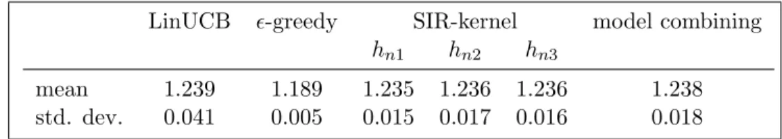
In addition to estimating the reward function for each arm, it is sometimes of interest to know which variables contribute to the reward for each arm, and some sparse dimen-sion reduction techniques can be applied. In particular, Chen et al. (2010) propose the coordinate-independent sparse estimation (CISE) to give sparse dimension reduction matrix such that the estimated coefficients of some predictors are zero for all reduction directions (i.e., some row vectors in ˆB_i,n∗ become0). When the SIR objective function is used, the corresponding CISE method is denoted by CIS-SIR. The numerical examples are given in the next chapter to show the performance of SIR and CIS-SIR.

2.4 Proofs

2.4.1 Proof of Theorem 2.1

Lemma 2.1. Suppose {Fj, j = 1,2,· · · }is an increasing filtration ofσ-fields. For each

j ≥ 1, let εj be an Fj+1-measurable random variable that satisfies E(εj|Fj) = 0, and

let Tj be anFj-measurable random variable that is upper bounded by a constant C >0

in absolute value almost surely. If there exist positive constants v and c such that for

(27)

n≥1, P n X j=1 Tjεj ≥n ≤exp− n 2 2C2_(v2₊_c/C) .

Proof of Lemma 2.1. Note that

P n X j=1 Tjεj ≥n ≤e−tnEhexpt n X j=1 Tjεj i =e−tnEhEexp t n X j=1 Tjεj |F_ni =e−tnEhexpt n−1 X j=1 Tjεj E(etTnεn_|F n) i .

By the moment condition on εn and Taylor expansion, we have

logE(etTnεn_|F n)≤E(etTnεn|Fn)−1 ≤tTnE(εn|Fn) + ∞ X k=2 tk|T_n|k k! E(|εn| k_|F n) ≤ v 2_C2_t2 2 (1 +cCt+ (cCt) 2₊_{· · ·}₎ = v 2_C2_t2 2(1−cCt) fort <1/cC. Thus, it follows by induction that

P n X j=1 Tjεj ≥n ≤exp−tn+ nv 2_C2_t2 2(1−cCt) ≤exp − n 2 2C2_(v2₊_c/C) ,

where the last inequality is obtained by minimization over t. This completes the proof of Lemma 2.1.

Lemma 2.2. Suppose {Fj, j = 1,2,· · · }is an increasing filtration ofσ-fields. For each

j ≥1, letWj be anFj-measurable Bernoulli random variable whose conditional success

probability satisfies

(28)

for some 0≤βj ≤1. Then given n≥1, P n X j=1 Wj ≤ n X j=1 βj /2≤exp−3 Pn j=1βj 28 .

Lemma 2.2 is known as an extended Beinstein inequality (see, e.g., Yang and Zhu (2002), section A.4.). For completeness, we give a brief proof here.

Proof of Lemma 2.3. Suppose ˜Wj, 1 ≤ j ≤n are independent Bernoulli random

vari-ables with success probability βj, and are assumed to be independent of Fj. By

Bern-stein’s inequality, P n X j=1 ˜ Wj ≤ n X j=1 βj /2≤exp−3 Pn j=1βj 28 .

Also, it is not hard to show that Pn

j=1Wj is stochastically no smaller than

Pn

j=1W˜j,

that is, for every t,P(Pn

j=1Wj > t)≥P(Pnj=1W˜j > t). Thus, Lemma 2.2 holds.

Lemma 2.3. Under the settings of the kernel estimation in section 2.3.1, given arm i

and a cube A ⊂ [0,1]d with side width h, if Assumptions 0, 2.3 and 2.4 are satisfied,

then for any >0,

P sup x∈A X j∈Ji,n+1 εjK x−X_j hn > n 1−1/√2 ≤ exp− n 2 4c2₄v2 + exp− n 4c4c + ∞ X k=1 2kdexp−2 k_n2 λ2_v2 + ∞ X k=1 2kdexp−2 k/2_n 2λc .

Proof of Lemma 2.3. At each time point j, let Wj = 1 if arm i is pulled (i.e., Ij =i),

and Wj = 0 otherwise. Denote G(x) = Pnj=1εjWjK( x−Xj

hn ). Then, to find an upper

bound for P(supx∈AG(x) > n/(1−1/

√

2)), we use a “chaining” argument. For each k ≥ 0, let γk =hn/2k, and we can partition the cube A into 2kd bins with bin width

γk. Let Fk denote the set consisting of the center points of these 2kd bins. Clearly,

card(Fk) = 2kd, andFkis aγk/2-net ofAin the sense that for everyx∈A, we can find

a x0 ∈ Fk such that kx−x0k ≤γk/2. Let τk(x) = argminx0_∈F

kkx−x

0_k _{be the closest}

point toxin the netFk. With the sequenceF0, F1, F2,· · · ofγ0/2, γ1/2, γ2/2,· · · nets in

(29)

Thus, by the continuity of the kernel function, we have limk→∞G(τk(x)) = G(x). It follows that G(x) =G(τ0(x)) + ∞ X k=1 G(τk(x))−G(τk−1(x)) . Thus, Psup x∈A G(x)> n 1−1/√2 =P sup x∈A G(τ0(x)) + ∞ X k=1 G(τk(x))−G(τk−1(x)) > ∞ X k=0 n 2k/2 ≤P sup x∈A G(τ0(x))> n + ∞ X k=1 P sup x∈A G(τk(x))−G(τk−1(x)) > n 2k/2 ≤Psup x∈F0 G(x)> n+ ∞ X k=1 P sup x2∈Fk, x1∈Fk−1 kx2−x1k≤γk/2 G(x2)−G(x1) > n 2k/2 ≤card(F0) max x∈F0 P G(x)> n + ∞ X k=1 2dcard(Fk−1) max x2∈Fk, x1∈Fk−1 kx2−x1k≤γk/2 PG(x2)−G(x1)> n 2k/2 , (2.4) where the last inequality holds because for eachx1 ∈Fk−1, there are only 2dsuch points

x2 ∈ Fk that can satisfy kx2 −x1k ≤ γk/2. Given x ∈ F0, since |WjK( x−Xj

h )| ≤ c4

almost surely for all j≥1, it follows by Lemma 2.1 that P G(x)> n≤exp − n 2 2c2₄(v2₊_c/c 4) . (2.5)

Similarly, given x2 ∈Fk,x1 ∈Fk−1 and kx2−x1k ≤γk, since

K x₂−X_j h −Kx1−Xj h ≤ λkx₂−x1k h ≤ λγk 2h = λ 2k+1

almost surely, it follows by Lemma 2.1 that P G(x2)−G(x1)> n 2k/2 =P _Xn j=1 jWj h K x₂−X_j h −K x₁−X_j h i > n 2k/2 ≤exp− 2 k+2_n2 2λ2_(v2_{+ 2}k/2+1_c/λ) . (2.6)

(30)

Thus, by (2.4), (2.5) and (2.6), P sup x∈A G(x)> n 1−1/√2 ≤ exp− n 2 2c2₄(v2₊_c/c 4) + ∞ X k=1 2kdexp− 2 k+2_n2 2λ2_(v2_{+ 2}k/2+1_c/λ) ≤ exp− n 2 4c2₄v2 + exp− n 4c4c + ∞ X k=1 2kdexp−2 k_n2 λ2_v2 + ∞ X k=1 2kdexp−2 k/2_n 2λc . This completes the proof of Lemma 2.3.

Proof of Theorem 2.1. Note that for each x∈Rd,

|fˆi,n+1(x)−fi(x)|= X j∈Ji,n+1 Yi,jK x−Xj hn X j∈Ji,n+1 K x−Xj hn −fi(x) = X j∈Ji,n+1 (fi(Xj) +εj)K x−Xj hn X j∈Ji,n+1 K x−Xj hn −fi(x) = X j∈Ji,n+1 (fi(Xj)−fi(x))K x−Xj hn X j∈Ji,n+1 K x−Xj hn + X j∈Ji,n+1 εjK x−Xj hn X j∈Ji,n+1 K x−Xj hn ≤ sup {x,y:kx−yk≤Lhn} |fi(x)−fi(y)|+ 1 Mi,n+1hdn X j∈Ji,n+1 εjK x−Xj hn 1 Mi,n+1hdn X j∈Ji,n+1 K x−Xj hn , (2.7)

where the last inequality follows from the bounded support assumption of kernel function K(·). By uniform continuity of the function fi,

lim

n→∞_{x,y_:_kx−yk≤Lhsup

n}

(31)

As a result, to show thatkfˆi,n−fik∞→0 as n→ ∞, we only need sup x∈[0,1]d 1 Mi,n+1hd X j∈Ji,n+1 εjK x−Xj h 1 Mi,n+1hd X j∈Ji,n+1 K x−Xj h →0 as n→ ∞. (2.8)

First, we want to show inf x∈[0,1]d 1 Mi,n+1hd X j∈Ji,n+1 K x−X_j h > c3cL d 1πn 2 , (2.9)

almost surely for large enough n. Indeed, for each n ≥ n0l+ 1, we can partition the

unit cube [0,1]dinto ˜B bins with bin widthL1hnsuch that ˜B ≤1/(L1hn)d. We denote

these bins by ˜A1,A˜2,· · ·,A˜_B˜. Given an arm i and 1 ≤ k ≤B˜, for every x ∈ A˜k, we

have X j∈Ji,n+1 K x−X_j hn = n X j=1 I(Ij =i)K x−X_j hn ≥ n X j=1 I(Ij =i, Xj ∈A˜k)K x−X_j hn ≥c3 n X j=1 I(Ij =i, Xj ∈A˜k),

where the last inequality follows by Assumption 2.4. Consequently, Pinf x∈_A˜_k 1 Mi,n+1hdn X j∈Ji,n+1 Kx−Xj hn ≤ c3cL d 1πn 2 ≤Pinf x∈A˜k 1 nhd n X j∈Ji,n+1 Kx−Xj hn ≤ c3cL d 1πn 2 ≤P c3 nhd n n X j=1 I(Ij =i, Xj ∈A˜k)≤ c3cLd1πn 2 =P _Xn j=1 I(Ij =i, Xj ∈A˜k)≤ cn(L1hn)dπn 2 . (2.10)

(32)

extended Bernstein inequality (Yang and Zhu, 2002, eq. 8) that P n X j=1 I(Ij =i, Xj ∈A˜k)≤ cn(L1hn)dπn 2 ≤exp−3cn(L1hn) d_π n 28 . (2.11) Therefore, P inf x∈[0,1]d 1 Mi,n+1hdn X j∈Ji,n+1 K x−X_j hn ≤ c3cL d 1πn 2 ≤ ˜ B X k=1 P inf x∈_A˜_k 1 Mi,n+1hdn X j∈Ji,n+1 K x−X_j hn ≤ c3cL d 1πn 2 ≤B˜exp−3cn(L1hn) d_π n 28 ,

where the last inequality follows by (2.10) and (2.11). With the conditionnh2dπ4_n/logn→ ∞, we immediately obtain (2.9) by Borel-Cantelli lemma.

By (2.9), it follows that (2.8) holds if sup x∈[0,1]d 1 Mi,n+1hdn X j∈Ji,n+1 εjK x−X_j hn =o(πn). (2.12) In the rest of the proof, we want to show that (2.12) holds. For each n≥n0l+ 1, we

can partition the unit cube [0,1]d intoB bins with bin length hn such that B ≤1/hdn.

At each time point j, letWj = 1 if armi is pulled (i.e.,Ij =i), andWj = 0 otherwise.

Then given >0, P sup x∈[0,1]d 1 Mi,n+1hdn X j∈Ji,n+1 εjK x−X_j hn > πn ≤B max 1≤k≤BP sup x∈Ak 1 Mi,n+1hdn X j∈Ji,n+1 εjK x−X_j hn > πn ≤BP M_i,n₊₁ n ≤ πn 2 +B max 1≤k≤BP sup x∈Ak 1 Mi,n+1hdn X j∈Ji,n+1 εjK x−X_j hn > πn, Mi,n+1 n > πn 2 ≤BPMi,n+1 n ≤ πn 2 +B max 1≤k≤BP sup x∈Ak X j∈Ji,n+1 εjK x−X_j hn > nπ_n2hd_n 2 ≤Bexp−3nπn 28 +B max 1≤k≤BP sup x∈Ak X j∈Ji,n+1 εjK x−X_j hn > nπ_n2hd_n 2 , (2.13)

(33)

where the last inequality follows by the extended Bernstein’s inequality. Note that by Lemma 2.3, P sup x∈Ak X j∈Ji,n+1 εjK x−X_j hn > nπ_n2hd_n 2 ≤2 exp −( √ 2−1)2nπ4_nh2_nd2 32c2 4v2 + 2 exp −( √ 2−1)nπ_n2hd_n 8√2c4c + 2 ∞ X k=1 2kdexp−( √ 2−1)22knπ4_nh2_nd2 8λ2_v2 + 2 ∞ X k=1 2kdexp−( √ 2−1)2k/2nπ2_nhd_n 4√2λc . (2.14) Thus, by (2.13), (2.14) and the condition that nh2_ndπ4_n/logn→ ∞, (2.12) is an immedi-ate consequence of Borel-Cantelli lemma. This completes the proof of Theorem 2.1. 2.4.2 Proofs of Theorem 2.2 and Corollary 2.2

Givenx∈[0,1]d, 1≤i≤landn≥n0l+1, defineGn+1(x) ={j: 1≤j ≤n, kx−Xjk ≤

Lhn} and Gi,n+1(x) = {j : 1 ≤ j ≤ n, Ij = i,kx−Xjk ≤ Lhn}. Let Mn+1(x) and

Mi,n+1(x) be the size of the setsGn+1(x) andGi,n+1(x), respectively. Then, the kernel

method estimator ˆfi,n+1(x) satisifes the following lemma.

Lemma 2.4. Suppose Assumptions 0, 2.1 and 2.4 are satisfied. Given x ∈ [0,1]d,

1≤i≤l and n≥n0l+ 1, for every > ω(Lhn;fi),

PXn |fˆ_i,n₊₁(x)−f_i(x)| ≥≤exp −3Mn+1(x)πn 28 +4Nexp−c 2 5Mn+1(x)πn −ω(Lhn;fi) 2 4c2 4v2+ 4c4c −ω(Lhn;fi) , (2.15)

wherePXn(·)denotes the conditional probability given design pointsXn= (X₁, X₂,· · · , X_n).

Proof of Lemma 2.4. It is clear that ifMn+1(x) = 0, (2.15) trivially holds. Without loss

of generality, assumeMn+1(x)>0. Define the eventBi,n={_M_i,n1₊₁₍_x₎Pj∈Ji,n+1K(

x−Xj

(34)

c5}. Note that PXn |fˆ_i,n₊₁(x)−f_i(x)| ≥ ≤PXn M_i,n₊₁(x) Mn+1(x) ≤ πn 2 +PXn |fî,n+1(x)−fi(x)| ≥, Mi,n+1(x) Mn+1(x) > πn 2 ≤exp −3Mn+1(x)πn 28 +PXn |fî,n+1(x)−fi(x)| ≥, Mi,n+1(x) Mn+1(x) > πn 2 , Bi,n +PXn |fî,n+1(x)−fi(x)| ≥, Mi,n+1(x) Mn+1(x) > πn 2 , B c i,n , =: exp −3Mn+1(x)πn 28 +A1+A2, (2.16)

where the last inequality follows by the extended Bernstein inequality. Under Bi,n, by

Assumption 2.4, the definition of the modulus continuity and the same argument as (2.7), we have |fˆi,n+1(x)−fi(x)|= P j∈Ji,n+1Yi,jK _x−X j hn P j∈Ji,n+1K _x−X j hn ≤ω(Lhn;fi) + 1 c5Mi,n+1(x) X j∈Gi,n+1(x) εjK x−X_j hn . Define ˜σt = inf{˜n : Pnj˜=1I(Ij = iand kx−Xjk ≤ Lhn) ≥ t}, t ≥ 1. Then, by the

previous display, for every > ω(Lhn;fi),

A1≤PXn X j∈Gi,n+1(x) εjK x−X_j hn ≥c5Mi,n+1(x) −ω(Lhn;fi) , Mi,n+1(x) Mn+1(x) > πn 2 ≤ N X ¯ n=0 PXn ¯ n X t=1 ε˜σtK x−X_σ_˜ t hn ≥c5n ¯ −ω(Lhn;fi) , Mi,n+1(x) Mn+1(x) > πn 2 , Mi,n+1(x) = ¯n ≤ N X ¯ n=dMn+1(x)πn/2e PXn ¯ n X t=1 εσ˜tK x−X_˜_σ t hn ≥c5¯n −ω(Lhn;fi) ≤ N X ¯ n=dMn+1(x)πn/2e 2 exp− nc¯ 2 5 −ω(Lhn;fi) 2 2c2 4v2+ 2c4c −ω(Lhn;fi) ≤2Nexp−c 2 5Mn+1(x)πn −ω(Lhn;fi) 2 4c2 4v2+ 4c4c −ω(Lhn;fi) , (2.17)

where the last to second inequality follows by Lemma 2.1 and the upper boundedness of the kernel function. By an argument similar to the previous two displays, it is not

(35)

hard to obtain that A2 ≤2Nexp −Mn+1(x)πn −ω(Lhn;fi) 2 4v2_{+ 4c}₋_ω(Lh n;fi) . (2.18)

Combining (2.16), (2.17), (2.18) and the fact that 0 < c5 ≤ 1 ≤ c4, we complete the

proof of Lemma 2.4.

Proof of Theorem 2.2. Since ˆf_i∗₍_X

n),n(Xn) ≤ fˆˆin,n(Xn), the regret accumulated after

the initial forced sampling period satisfies that

N X n=n0l+1 f∗(Xn)−fIn(Xn) = N X n=n0l+1 fi∗₍_X n)(Xn)−fî∗(Xn),n(Xn) + ˆfi∗(Xn),n(Xn)−fîn(Xn) +fîn(Xn)−fIn(Xn) ≤ N X n=n0l+1 f_i∗₍_X n)(Xn)−fî∗(Xn),n(Xn) + ˆfîn,n(Xn)−fîn(Xn) +fîn(Xn)−fIn(Xn) ≤ N X n=n0l+1 2 sup 1≤i≤l |fî,n(Xn)−fi(Xn)|+AI(In6= în) . (2.19)

It can be seen from (2.19) that the error upper bound consists of the estimation error regret and randomization error regret.

First, we find the upper bound of the estimation error regret. Given armi,n≥n0l

and > ω(Lhn;fi), P|fˆi,n+1(Xn+1)−fi(Xn+1)| ≥ ≤EPXn+1 Mn+1(Xn+1)≤ cn(2Lhn)d 2 +EP_Xn+1 |fˆi,n+1(Xn+1)−fi(Xn+1)| ≥, Mn+1(Xn+1)> cn(2Lhn)d 2 . (2.20) Since for every x∈[0,1]d,P(kx−Xjk ≤Lhn)≥c(2Lhn)d, 1 ≤j ≤n, we have by the

extended Bernstein’s inequality that PXn+1 Mn+1(Xn+1)≤ cn(2Lhn)d 2 ≤exp −3cn(2Lhn) d 28 . (2.21)

(36)

By Lemma 2.4, PXn+1 |fˆi,n+1(Xn+1)−fi(Xn+1)| ≥, Mn+1(Xn+1)> cn(2Lhn)d 2 ≤exp −3cn(2Lhn) d_π n 56 + 4Nexp −c 2 5cn(2Lhn)dπn −ω(Lhn;fi) 2 8c2₄v2_{+ 8c} 4c −ω(Lhn;fi) . (2.22) Let ˜ i,n=ω(Lhn;fi) + s 16c2₄v2_log(8lN2_/δ) c2₅c(2L)d_nhd nπn .

Then, by (2.20), (2.21), (2.22) and the definition ofnδ in (2.2), it follows that for every

n≥nδ, P |fˆi,n+1(Xn+1)−fi(Xn+1)| ≥˜i,n ≤ δ 4lN + δ 4lN + δ 2lN = δ lN, which implies that

P _XN n=nδ+1 2 sup 1≤i≤l |fˆi,n(Xn)−fi(Xn)| ≥ N X n=nδ+1 2 max 1≤i≤l˜i,n−1 ≤δ. (2.23) Next, we want to bound the randomization error regret. Given >0, sinceP(In6=

ˆ_i_n_{) = (l}₋_1)π_n_{, we have by Hoeffding’s inequality that}

PA N X n=nδ+1 I(In6= ˆin)− N X n=nδ+1 (l−1)πn ≥≤exp− 2 2 N A2 .

Taking =ApN/2 log(1/δ), we immediately get P A N X n=nδ+1 I(In6= ˆin)≥ N X n=nδ+1 (l−1)πn+A r N 2 log 1 δ ≤δ. (2.24) Then, (2.19), (2.23) and (2.24) together complete the proof of Theorem 2.2.

(37)

Chapter 3

Model Combining Based

Allocation

In this chapter, based on the allocation strategy described in section 4.1 of the previ-ous chapter, we consider the general case that multiple candidate function estimation methods are used for model combining. First, we study the strong consistency of the algorithm. Then we evaluate the numerical performance with both simulation and a web-based real dataset.

3.1 Strong Consistency

We consider the general case that multiple function estimation methods are used for model combining. It is known from section 2.3 that strong consistency in L∞ norm is

desirable for the randomized allocation strategy. However, it is often technically difficult to verify strong consistency in L∞norm for a regression method. Also, practically, It is

likely that some methods may give good estimation for only a subset of the arms, but performs poorly for the rest. Not knowing which methods work well for which arms, we propose the combining algorithm to addresses this issue. We will show that even in the presence of bad-performing regression methods, the strong consistency of our allocation strategy still holds if for any given arm, there is at least one good regression method included.

Given an arm i, let N_t(i) = inf

n: Pn

j=n0l+1I(Ij =i) ≥ t , t ≥1, be the earliest

(38)

time point where arm iis pulled exactly t times after the forced sampling period. For notation brevity, we use Nt instead of Nt(i) in the rest of this section. Consider the

assumptions as follows.

Assumption A. Given any arm 1 ≤ i≤ l, the candidate regression procedures in ∆

can be categorized into one of the two subsets denoted by ∆i1 (non-empty) and ∆i2. All

procedures in ∆i1 are strongly consistent in L∞ norm for arm i, while procedures in

∆i2 are less well-performing in the sense that for each procedure δs in ∆i2, there exist

a procedure δr in ∆i1 and some constants b >0.5, c1>0 such that

lim inf T→∞ T X t=1 ˆ fi,Nt,s(XNt)−fi(XNt) 2 − T X t=1 ˆ fi,Nt,r(XNt)−fi(XNt) 2 √ T(logT)b > c1 with probability one.

Assumption B. The mean functions satisfy A= sup₁≤i≤lsupx∈[0,1]d(f∗(x)−f_i(x))<

∞.

Assumption C. kfˆi,n,r −fik∞ is upper bounded by a constant c2 for all 1 ≤ i ≤ l,

n≥n0l+ 1and 1≤r≤m.

Assumption D. The variance estimatesvˆi,nare neither too close to zero nor too large:

there exist constants 0< p < q <∞ such that

p≤vˆi,n≤q

with probability one for all 1≤i≤l and n≥n0l+ 1.

Assumption E. The sequence {πn, n≥1} satisfies that P∞n=1πn diverges.

Note that Assumption A is automatically satisfied if all the regression methods happen to be strongly consistent (i.e., ∆i2 is empty). When a bad-performing method

does exist, Assumption A requires that the difference of the mean square errors between a good-performing method and a bad-performing method decreases slower than the order of (logT)b/√T. If a parametric method δs in ∆ is based on a wrong model,

PT

t=1 fˆi,Nt,s(XNt)−fi(XNt)

2

is of order T, and then the requirement in Assumption A is met. For an inefficient nonparametric method, the enlargement of the mean square

(39)

error by the order larger than (logT)b/√T is natural to expect. Assumption B is a natural condition in the context of our bandit problem. If the mean reward functionsfi’s

are continuous, Assumptions C can be satisfied by applying a truncation method on the function estimator. Similarly, Assumption D is satisfied by truncating the “combined” variance estimate ˆvi,n to be inside a positive interval. Assumption E ensures that Nt

is finite as shown in Lemma 3.1 in the Appendix. As implied in Lemma 3.1, if we are allowed to play the game infinitely many times, each arm will be pulled beyond any given integer. This guarantees that each “inferior” arm can be pulled reasonably often to ensure enough exploration.

Theorem 3.1. Under Assumption 0 and Assumptions A-E, the model combining allo-cation strategy is strongly consistent.

With Theorem 3.1, one is safe to explore different models or methods in estimating the mean reward functions that may or may not work well for some or all arms, as long as the candidates are properly combined. The resulting per-round regret can be much improved if good methods (possibly different for different arms) are added in.

3.2 Simulations

For simulations, two examples with a univariate covariate are shown in section 3.2.1, and a more complicated example for multivariate covariates with the application of dimension reduction is given in section 3.2.2.

3.2.1 Univariate Covariate

The first case presented here has nonlinear reward functions with normal random er-rors, while the second case has binary responses with both linear and nonlinear reward functions.

(40)

Case 1

Consider a bandit problem with two arms. Suppose the true mean reward functions of the two arms on [0,1] are

f1(x) = 2e−200(x−0.2) 2 + 2e−200(x−0.8)2, f2(x) = 0.5x2+e−(x−0.5) 2 .

It is clear that no arm dominates the other over the entire domain [0,1], and the optimal decision should be made based on the value of the covariate. Given the time horizon N = 800, assume that for 1 ≤ n≤ N, the covariates are sampled from uniform(0,1), and the errors εn are normally distributed with mean 0 and variance σ2= 0.5. Let the

first 20 rounds of the game be the initial forced sampling period.

We start with the Nadaraya-Watson regression described in section 2.3.1. Here we use the Epanechnikov quadratic kernel

K(t) =    3 4(1−t 2₎ _if_{|t| ≤}_1; 0 otherwise.

For illustration, we consider three bandwidth choices: h1 = _(log 1

2n)0.25, h2 =

1 log2n and

h3 = _(log1

2n)2. Treating these three choices as different candidate modeling procedures,

we run the model combining allocation strategy with the “inferior” arm sampling prob-ability πn = _log1

2n to obtain the per-round regret rn and the inferior sampling rate

qn. For comparison, each of the bandwidth choices is also run separately with the

al-location strategy. We repeat this process 20 times to obtain the averaged per-round regret ¯rnand the averaged inferior sampling rate ¯qn, and plot the resulting ¯rnand ¯qn in

Figure 3.1. We can see that in this case, the combining strategy performs even better than the winner of the three candidate procedures. It is also interesting to compare the weights of the three candidate procedures in the combining strategy at different rounds of the game (Table 3.1). As expected, the weights for a given arm can evolve as more and more rounds are played. We can also see that given n, the dominating candidate procedures are not necessarily the same for the two arms. Therefore, it supports that the model combining algorithm enables the allocation strategy to smartly evolve and appropriately prefer the better estimation methods for different arms at different time points to achieve an optimal performance.

(41)

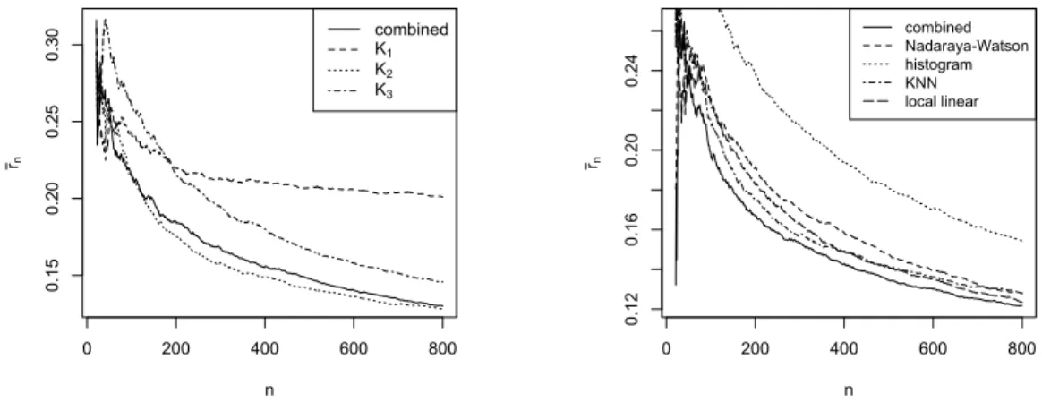
0 200 400 600 800 0.15 0.20 0.25 0.30 n rn combined h1 h2 h3 0 200 400 600 800 0.15 0.20 0.25 0.30 0.35 0.40 n qn combined h1 h2 h3

Figure 3.1: (Case 1) Combining Nadaraya-Watson regressions with different bandwidth choices. Left panel: averaged per-round regret. Right panel: averaged inferior sampling rate.

Table 3.1: (Case 1) Weights of bandwidth choices for Nadaraya-Watson regressions from the last repeat

arm 1 arm 2

bandwidth h1 h2 h3 h1 h2 h3

weight (n= 40) 0.00 0.00 1.00 0.26 0.65 0.09 weight (n= 800) 0.00 0.00 1.00 0.03 0.97 0.00

As another example, we use theK-nearest neighbor method withK1 =b_(log n

2n)0.25

c, K2 = b_logn

2nc and K3 = b

n

(log2n)2c, and repeat the simulation study described above.

The averaged per-round regret in Figure 3.2 (left panel) shows that the performance of the combining strategy is satisfactorily close to the best of the three choices of K. Since the graphs for averaged inferior sampling rate look very similar to that of averaged per-round regret, we only present the graphs for per-per-round regret in the following numerical examples.

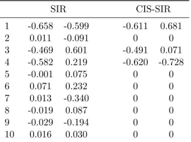
Next, we combine different nonparametric methods. Consider the following four nonparametric methods with the specified tuning parameters: histogram method with

(42)

0 200 400 600 800 0.15 0.20 0.25 0.30 n rn combined K1 K2 K3 0 200 400 600 800 0.12 0.16 0.20 0.24 n rn combined Nadaraya-Watson histogram KNN local linear

Figure 3.2: (Case 1) Averaged per-round regret from combining different methods. Left panel: combiningK-nearest neighbor methods with different choices ofK. Right panel: combining different nonparametric methods.

the bin width _b_(log1

2n)2c, Nadaraya-Watson regression with the kernel bandwidth

1 (log2n)2,

local linear regression with the kernel bandwidth _log1

2n andK-nearest neighbor method

with K = b n

log2nc. Repeat the simulation study under the same settings as described

above, and the summary plot is shown in Figure 3.2 (right panel). Again, the combining strategy performs very well compared with the individual candidate procedures. Case 2

Consider a two-armed bandit problem with 0-1 binary responses. Suppose the true reward functions (i.e.,P(Y = 1|X =x)) of the two arms on [0,1] are

f1(x) = 0.7e−30(x−0.2)

2

+ 0.7e−30(x−0.8)2, f2(x) = 0.65−0.3x.

Except for the mean reward functions and the error distribution, the settings of case 2 remain the same as case 1. Clearly, the error distribution here is dependent on the covariate. For combining modeling methods, we consider Nadaraya-Watson regression with bandwidth h1 = _log1

2n and h2 =

1

(log2n)2. In addition, we intentionally add linear

(43)

for estimating arm 1, and is expected to perform poorly. The model combining strategy as well as the individual modeling candidates are repeated 50 times. By examining the weights of the combining strategy for the last run in Table 3.2, we can see that for arm 1, the linear regression is eventually assigned a very small weight while the Nadaraya-Watson regression with better bandwidth choice stands out. On the other hand, arm 2 seems to prefer the linear regression, which can be more efficient in estimating the linear mean reward function. The summary plot in Figure 3.3 (left panel) confirms that linear regression alone gives rather poor results, while the combining strategy once again performs very closely to the best individual modeling candidate.

Table 3.2: (Case 2) Weights for combining Nadaraya-Watson (NW) regression and linear regression

arm 1 arm 2

bandwidth NW-h1 NW-h2 linear reg. NW-h1 NW-h2 linear reg.

weight (n= 40) 0.10 0.78 0.12 0.20 0.00 0.80 weight (n= 800) 1.00 0.00 0.00 0.00 0.00 1.00 0 200 400 600 800 0.04 0.05 0.06 0.07 0.08 0.09 n rn combined Nadaraya-Watson-h1 Nadaraya-Watson-h2 linear regression 200 400 600 800 1000 1200 0.02 0.04 0.06 0.08 0.10 0.12 n rn combined SIR CIS-SIR

Figure 3.3: Averaged per-round regret from combining different methods. Left panel: (Case 2) combining Nadaraya-Watson regression and linear regression. Right panel: (the multivariate covariate case) comparing SIR and CIS-SIR.

(44)

3.2.2 Multivariate Covariates with Dimension Reduction

In this subsection, we use the dimension reduction function estimation procedures de-scribed in section 2.3.3 for bandit problem with multivariate covariates. Two readily available MATLAB packages for dimension reduction are used: LDR package (Cook et al., 2011) for SIR, and CISE package (Chen et al., 2010) for CIS-SIR. The kernel used is the Gaussian kernel

K(t) = exp(−ktk

2 2

2 ).

We consider a three-arm bandit model with d= 10. Assume that at each time n, the covariate is Xn = (Xn1, Xn2,· · · , Xnd)T, and Xni’s (i= 1,· · · , d) are i.i.d random

variables from uniform(0,1). Assume the error n ∼ 0.5N(0,1). Consider the mean

reward functions f1(Xn) =0.5(Xn1+Xn2+Xn3), f2(Xn) =0.4(Xn3+Xn4)2+ 1.5 sin(Xn1+ 0.25Xn4), f3(Xn) = 2Xn3 0.5 + (1.5 +Xn3+Xn4) .

We set the reduction dimensions for the three arms by r1 = 1, r2 = 2 and r3 = 2.

Given the time horizonN = 1200, the first 90 rounds of the game are the forced sampling period. Let the “inferior” arm sampling probability be πn = _(log1

2n)2, and the kernel

bandwidth for arm ibe h =n−1/(2+ri)_, _i_{= 1,}_2,_{3. Dimension reduction methods SIR,}

CIS-SIR as well as their combining strategy are run separately, and their per-round regret rn is summarized in Figure 3.3 (right panel), which shows that the combining

strategy performs the best. Since the second arm (i= 2) is played the most (for SIR, 1022 times; for CIS-SIR, 1026 times), we show the estimated dimension reduction matrix for the second arm at the last time point n= N in Table 3.3. As expected, CIS-SIR results in a sparse dimension reduction matrix with rows 1, 3 and 4 being non-zero.

3.3 Web-Based Personalized News Article

Recommenda-tion

In this section, we use the Yahoo! Front Page Today Module User Click Log dataset (Ya-hoo! Academic Relations, 2011) to evaluate the proposed allocation strategy. The

(45)

Table 3.3: Comparing the estimated dimension reduction matrix ˆB₂∗_,N for the second arm between SIR and CIS-SIR.

SIR CIS-SIR 1 -0.658 -0.599 -0.611 0.681 2 0.011 -0.091 0 0 3 -0.469 0.601 -0.491 0.071 4 -0.582 0.219 -0.620 -0.728 5 -0.001 0.075 0 0 6 0.071 0.232 0 0 7 0.013 -0.340 0 0 8 -0.019 0.087 0 0 9 -0.029 -0.194 0 0 10 0.016 0.030 0 0

complete dataset contains about 46 million web page visit interaction events collected during the first ten days in May 2009. Each of these events has four components: (1) five variables constructed from the Yahoo! front page visitor’s information; (2) a pool of about 10-14 editor-picked news articles; (3) one article actually displayed to the visitor (it is selected uniformly at random from the article pool); (4) the visitor’s response to the selected article (no click: 0, click: 1). Since different visitors may have different preferences for the same article, it is reasonable to believe that the displayed article should be selected based on the visitor associated variables. If we treat the articles in the pool as the bandit arms, and the visitor associated variables as the covariates, this dataset provides the necessary platform to test a MABC algorithm.

One remaining issue before algorithm evaluation is that the complete dataset is long-term in nature and the pool of articles is dynamic, i.e., some outdated articles are dropped out as people’s interest in these articles fades away, and some breaking-news articles can appear and be added to the pool. Our current problem setup, however, assumes stationary mean reward functions with a fixed set of arms. To avoid introducing biased evaluation results, we focus on short-term performance where people’s interest on a particular article does not change too much and the pool of articles remains stable. Therefore, we consider only one day’s data (May 1, 2009). Also, we choose four articles

Nonparametric Estimation and Model Combination in a Bandit Problem with Covariates