spike train data with application to
multi-electrode array recordings.
Siti Noormiza Binti Makhtar
PhD
University of York
Electronic Engineering
Abstract
This thesis proposes a novel approach for functional connectivity studies of neu-ronal signal recordings based on statistical signal processing analysis in the fre-quency domain using Multivariate Partial Coherence (MVPC) combined with network theory measures. MVPC is applied to spike trains signals to make in-ferences about the underlying network structure. The presence of connections between single unit spike trains is estimated using both coherence and MVPC analysis. Scalability of MVPC analysis is investigated through application to sim-ulated spike train data with up to 100 simultaneous spike trains generated from a network of excitatory and inhibitory cortical neurons. Stable MVPC estimates were obtained with up to 198 predictors in partial coherence estimates, using a combination of simulated cortical neuron data and additional Poisson spike train predictors. MVPC provides higher order partial coherence analysis for multi-channel spike trains signals, removing effects of common influences in pairwise connectivity estimates. Network measures applied to binary and weighted adja-cency measures derived from coherence and partial coherence are compared to determine the differences in unconditional and conditional networks of spike train interactions. A combination of MVPC analysis along with network theory anal-ysis provides a systematic approach for multi-channel spike train signals. The proposed method is applied to simulated and multi-electrode array (MEA) spike train data. The MEA data consists of 19 single unit channels recorded from a study of connectivity in a model of kainic acid (KA) induced epileptiform activity for mesial temporal lobe epilepsy (mTLE) in rat. The network theory analysis uses basic measures on both conditional and unconditional network, which high-lights the differences in network structure and characteristics between the two representations. Complex analysis on conditional networks is useful in describing the properties of integration and segregation in the network.
Abstract 2 List of Figures 4 List of Tables 12 Acknowledgments 14 Author’s declaration 15 1 Introduction 16 1.1 Motivation . . . 18 1.2 Objectives . . . 19 1.3 Thesis Outline . . . 19 2 Literature Review 22 2.1 Brain levels of organization . . . 23
2.2 Neurons . . . 26
2.2.1 Local potentials . . . 27
2.2.2 Action potentials . . . 29
2.2.3 Synaptic signalling . . . 31
2.2.4 Dendritic processing . . . 34
2.3 Spiking neuron models . . . 36
2.3.1 Hodgkin-Huxley model . . . 37
2.3.2 Integrate-and-Fire neuron model . . . 41
2.3.3 Izhikevich model . . . 44
2.3.4 Cortical network model . . . 45
2.4 Neuronal signals recording . . . 46
2.4.1 Single unit recordings . . . 47
2.4.2 MEA recordings . . . 49
2.5 Spikes detection in MEA signals . . . 50
2.6 Functional connectivity analysis. . . 51
2.7 Chapter summary . . . 57
3 Spectral Analysis 59 3.1 Spectral estimation . . . 60
3.2 Cross spectral estimation . . . 61
3.3 Coherence analysis . . . 62
Contents 4
3.4 Partial coherence analysis . . . 64
3.5 Higher order partial coherence analysis . . . 65
3.6 Multivariate partial coherence analysis . . . 66
3.7 Chapter summary . . . 71
4 Network Theory and Metrics 72 4.1 Network measures applied to neuronal interactions . . . 73
4.1.1 Degree . . . 76
4.1.2 Path length and network efficiency . . . 77
4.1.3 Clustering coefficient . . . 79
4.1.4 Modularity . . . 80
4.2 Network motifs . . . 81
4.3 Network small-worldness . . . 83
4.4 Chapter summary . . . 85
5 Spiking neuronal network model: Network measures analysis 86 5.1 Neuronal networks configuration . . . 87
5.2 Scalability test for MVPC analysis . . . 91
5.3 Conditional and unconditional network analysis . . . 97
5.3.1 Node degree analysis on simulated network. . . 101
5.3.2 Path length analysis on simulated network. . . 103
5.4 Reproducibility of network motifs . . . 111
5.5 Small world analysis: Binary and weighted network analysis . . . 116
5.6 Chapter summary . . . 117
6 Application of network theory metrics to MEA epileptic seizure data 121 6.1 MEA data set-single unit spike train data from hippocampus . . . 122
6.2 Node degree . . . 131
6.3 Path length . . . 135
6.4 MEA: Clustering coefficient . . . 140
6.5 MEA: Small-world network . . . 142
6.6 MEA: Modularity . . . 144
6.7 Chapter summary . . . 146
7 Conclusions and Further Work 148 7.1 General Summary . . . 148
7.2 Chapter Summaries and Conclusions . . . 149
7.3 Future work . . . 152
A 155 A.1 Neuronal parameters for cortical network model . . . 156
A.2 Frequency of subgraphs in Network A . . . 157
2.1 Lateral surface of the cerebral hemisphere. Major regions of the brain: frontal, parietal, occipital and temporal lobes. Cerebel-lum is considered part of the motor system. ( Figure from http: //commons.wikimedia.org/ ) . . . 23 2.2 Levels of organization in the central nervous system differentiated
by spatial scales. (Figure from Trappenberg (2010)) . . . 24 2.3 The fifty two subregions based on cellular morphology and
organi-zation by Brodmann. (Gazzaniga et al., 1998) . . . 26 2.4 Schematic view of a typical neuron. ( Figure from http:
//com-mons.wikimedia.org/ ) . . . 27 2.5 Ions moving across plasma through (a)The ion channel allows
spe-cific type of ions to flow across the channel, and (b)ion pumps maintain balance ions concentrations inside and outside the cell by forcing the ions to move against their concentration gradients when ion pumps break adenosine triphosphate, ATP into energy. (Figure from Elmslie (2001)) . . . 28 2.6 Schematic diagrams of the axon equivalent circuit. RM,membrane
resistance;RI, intracellular resistance;CM, membrane capacitance.
(Figure from Kandel et al. (2000)) . . . 29 2.7 The trace shows depolarization and repolarization of the
mem-brane potential. Depolarization phase occur when Na+ ions enter
the cell and decrease the internal ions negativity until the num-ber of Na+ ions entering the cell are more than the number of K+ ions leaving the cell. Repolarization phase occur when the mem-brane permeability towards K+ is increase and cause a flow of K+
ions leaving the cell. Finally, inactivation of K+ channels shifts the membrane potential to the initial resting state. (Figure from Freeman, 2005) . . . 30 2.8 Synaptic signalling is initiated by electrical signalling followed by
chemical event between neurons and finally producing excitatory postsynaptic potential (EPSP) or inhibitory postsynaptic potential (IPSP). (From Purves et al. (2008)) . . . 32 2.9 (A) Glutamat-induced EPSP generated when reversal potential,
Erev is more positive than the action potential threshold. (B)
GABA-induced IPSP generated when Erev is more negative than
the action potential threshold. (Figure adapted from Purves et al. (2008)) . . . 33
List of Figures 6
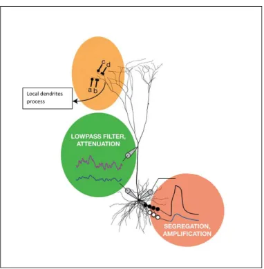
2.10 High amplitude of EPSP generated at the synapse location will reduce after an attenuation results in lower amplitude of EPSPs at the soma. ( Figure from Williams & Stuart (2002) ) . . . 35 2.11 Y ellow : Local nonlinear dendritic integration. Green : Longer
dendritic pathway significantly attenuate EPSPs signal. Brown: Integration at the cell body followed by comparison against thresh-old level before firing an action potential. ( Figure edited from London & H¨ausser (2005) ) . . . 36 2.12 Representation of an equivalent electrical circuit for Hodgkin-Huxley
model. This circuit includes a capacitor, two variable resistors to represent voltage-dependant conductances, a static resistor to rep-resent small leakage current and a battery for each channel. (From Trappenberg (2010)) . . . 38 2.13 (A) The equilibrium functions ( X0 = probability for activation
and inactivation events ) and (B) time constants ( in unit of msec) for variables n, m and h in HH model. ( Membrane potential in unit of mV ) (Figure from Trappenberg (2010)) . . . 40 2.14 Membrane potential of HH model shows a constant firing rate spike
train initiated by constant external current with sufficient strength. (From Trappenberg (2010)) . . . 41 2.15 Integrate-and-fire neuron model integrates n input channels
writ-ten as an α-function multiplied by a synaptic strength value wj.
An action potential will be fired when the total input potential reach a firing threshold. (Edited from Trappenberg (2010) . . . . 42 2.16 This figure illustrates a low-pass filter circuit at synapse location to
filter presynaptic currentδ(t−tfj) producing an input current pulse,
α(t−tf
j). The generated input current pulse will be attenuated to
the soma. The IF model equivalent circuit in the soma consists of a reistor, R and a capacitor, C. The capacitor will be charged by the input current, I(t). An output pulse, δ(t−tf
i) is generated
at timetf
i when the voltage across capacitance increases and reach
the threshold voltage, ϑ. (From Gerstner & Kistler (2002)) . . . . 43 2.17 Output voltage of IF model with a threshold voltage, ϑ = 10mV.
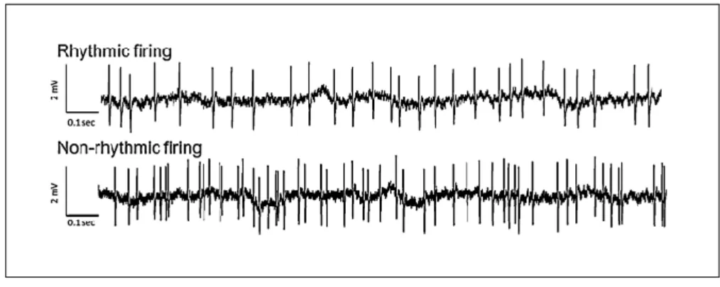
(A) Constant current input with strength less than threshold age. (B) Constant input with strength greater than threshold volt-age generating a spike train shown by dots in the upper figure. (From Trappenberg (2010)) . . . 44 2.18 An example of signals recorded using glass electrode showing
rhyth-mic neuronal firing and non-rhythrhyth-mic neuronal firing. (From Gan-drathi et al. (2013) . . . 48 2.19 An example of single unit activity of neuron recorded using
micelec-trode wire (black traces). Green circles show spikes event filtered using thresholding procedures. (Figure from David et al. (2010)) . 49
2.20 Intrinsic firing pattern of A) regular spiking neuron(top trace) in response to intracellular stimulation of prolonged depolarizing cur-rent (bottom trace) and B) fast spiking neuron (top trace) in re-sponse to the same stimulus current (bottom trace). (From Con-nors & Gutnick (1990)) . . . 51 2.21 Step by step of spike sorting methods; i) Signals filtering using
band-pass filter. ii) Spikes detection using specified amplitude threshold. iii) Feature extraction to distinguish different features of the spikes. iv) Clustering to classify the signals into individual neuron spikes. (From Quiroga (2007)) . . . 52 2.22 Framework for estimation of pairwise neuronal interactions and
connectivity analysis on MEA and simulated spike train signals. . 57 4.1 Binary and weighted network examples for Ab (left) in Eq. 4.1
andAw (right) in Eq. 4.2. In the binary case the edge between two
nodes is indicated by a line to indicate the presence of a connection from node i to node j. The strength of connection between two nodes can be represented by various thickness of the edge lines as shown in the weighted network (right). . . 75 4.2 A regular network (left) shows similar pattern of synchronized
in-teractions across the entire network and a random network (right) shows random connections across a network with non-existence of specific pattern of interactions. Both regular and random networks consist of 20 nodes with an average of 4 connections per node. . . 76 4.3 Six possible sub-network patterns with undirected motifs ID: h1,
h2, h3, h4, h5 and h6 from motif size, M = 4. . . 82
4.4 This figure show (a) a regular network with high values of C and
L, (b) a small world network with optimum connections with co-existence of segregation and integration properties represent high
C and low L, and (c) a random network with low values ofC and
L. All of these networks consist of 20 nodes with an average degree of 4 connections per node. . . 84 5.1 2D planar sheet connectivity for simulation of excitatory (left) and
inhibitory (right) neuron. Each character indicates the position of a neuron in Network A. ’O’ is the presynaptic neuron, ’+’ are the postsynaptic neurons receiving excitatory inputs from ’O’, ’−’ are the postsynaptic neurons receiving inhibitory inputs from ’O’ and ’•’ are other neurons not receiving any input from ’O’. Designation of excitatory or inhibitory neuron for 2D connectivity in Network A is presented in figure 5.2. . . 89 5.2 Positions of excitatory and inhibitory neurons for simulation of
Network A. Blue dots are the excitatory neurons and red dots are the inhibitory neurons. X and Y indicate the positions of neurons for pairwise connectivity analysis using different numbers of predictors in section 5.2. . . 89
List of Figures 8
5.3 Network B is a model of small-world network generated with rewiring probability of 0.05 (Watts & Strogatz, 1998). This network consists of 200 nodes that adopts similar connectivity pattern of excitation and inhibition. . . 90 5.4 Left column: histogram plot for the (a) output firing rates and (c)
output COV for model A of 100 neurons. Right column: histogram plot for the (b) output firing rates and (d) output COV for model B of 200 neurons. . . 91 5.5 Figure shows different partial coherence values from MVPC
anal-ysis on 100 spike trains with different data lengths, 100 sec, 200 sec and 300 sec. Original coherence is included for comparison. Partial coherence should be less than or equal to ordinary coher-ence.Longer data lengths generate stable MVPC analysis. . . 92 5.6 Figure shows position of 10 predictor neurons located around
neu-rons X and Y. Blue dots show the excitatory neuneu-rons and red dots show the inhibitory neurons. . . 93 5.7 Figure shows comparison between coherence and partial coherence
values after gradually increasing the number of predictors from 1 to 10 neurons located around neurons X and Y as shown in Figure 5.6. 94 5.8 Figure (a) to (d) show neurons X and Y positioned in the middle
of 2D network with the predictors highlighted in the green boxes. Blue dots show the excitatory neurons and red dots show the in-hibitory neurons. . . 95 5.9 Figure shows comparison between coherence and partial coherence
values after gradually increasing the number of predictors for pair-wise interaction between neurons X and Y. . . 96 5.10 Figure shows comparison between coherence and partial coherence
values after gradually increasing the number of predictors around neurons X and Y, with combination of additional 100 poisson spike trains. . . 98 5.11 Unconditional weighted network for simulated Network A with
excitatory neurons (red) and inhibitory neurons (green). Links between nodes show weighted edges constructed from coherence analysis. Thicker edges show stronger connections. . . 99 5.12 Conditional weighted network for simulated Network A with
ex-citatory neurons (red) and inhibitory neurons (green). Links be-tween nodes show weighted edges constructed from multivariate partial coherence analysis. Thicker edges show stronger connections.100
5.13 Top figure shows position of nodes using number 1 to 100 for sim-ulated Network A. Blue and red circle distinguish between exci-tatory and inhibitory neurons, respectively. Middle figure shows color-coded graph of conditional node degree for Network A, and bottom figure shows the unconditional node degree for Network A. The values of degree for each nodes middle and bottom plots are ar-ranged according to neurons positions as shown in top figure. Un-conditional network shows high number of connections compared to the conditional network. Unconditional node degree range are higher between 6 to 80, compare to the conditional degree. Top figure clearly shows reduction in conditional node degree. Elimi-nation of common effects reduces node degree in the range of 2 to 13 in conditional network as expected according to the simulated model of Network A. . . 102 5.14 Color-coded graphs of binary path length for unconditional
net-work. Position of nodes is according to Figure 5.13(top). . . 106 5.15 Color-coded graphs of binary path length for conditional network.
Position of nodes is according to Figure 5.13(top). . . 106 5.16 Color-coded graphs of weighted path length for unconditional
net-work. Position of nodes is according to Figure 5.13(top). . . 107 5.17 Color-coded graphs of binary path length for conditional network.
Position of nodes is according to Figure 5.13(top). . . 107 5.18 Binary and weighted path length distributions for unconditional
and conditional connectivity of Network A. . . 108 5.19 Color-coded graphs of binary unconditional path length(top) and
conditional path length(bottom) to show the shortest distance from neuron 1 to all other neurons in Network A according to the neurons position in Figure 5.13(top). Neuron 1 located at the top left of both graphs in dark blue color. Realistic distance can be seen in conditional path length, for example the highest path length is the distance to neuron 100 at the bottom right of the graph.109 5.20 Color-coded graphs of weighted unconditional path length(top)
and conditional path length(bottom) to show the weighted shortest distance from neuron 1 to all other neurons in Network A according to the neurons position in Figure 5.13(top). Weighted conditional path length in this graph is consistent with binary conditional path length in Figure 5.19 with gradual increment in the distance from Neuron 1 to all other neurons according to the location of the neuron. Weighted path length is also affected by the strength of interactions between neurons contributed by the neuronal excita-tory and inhibiexcita-tory activities. . . 110 5.21 The expected pattern for subgraph connecting 6 excitatory neurons
with maximum number of edges according to Figure 5.1(left). . . 114 5.22 Conditional weighted network for simulated Network B. Links
be-tween nodes show weighted edges constructed from MVPC analy-sis. Thicker edges show stronger connections between nodes. . . . 118
List of Figures 10
5.23 Unconditional network for simulated Network B. This network does not exhibit SWN properties as expected for Network B. . . . 119 6.1 Simultaneous recordings of multiple hippocampal neuronal
activ-ity. This trace illustrates a sample representation of spontaneous hippocampal unit firing observed over a 600 sec. The colours of the raster represent the firing rate of the neurons ranging from black (slow), red (medium) and yellow (high). . . 123 6.2 Shape and size of the principle neurons in the Dentate Gyrus, CA1
and CA3. Number indicate the dendritic length of the cells. Figure from Shepherd (1990) . . . 124 6.3 A: Schematic representation of the hippocampal recording sites. B:
Histological verification of hippocampal recording sites with elec-trode placement was confirmed by the visible blue dye mark. . . 125 6.4 Time-line experimental protocols for kainic acid administration.
Saline was injected intravenously after 10 min baseline recording followed by local injection of KA after 20 min saline injection. Effect of KA was recorded until 210 minute. . . 126 6.5 Unconditional weighted network for bilateral hippocampal single
unit dataset at four different stages: a) baseline, b) saline injection, c) KA injection and d) effect of KA. Different nodes color show different subregions of the hippocampus; orange - CA3 Left, blue - CA1 Left, green - CA3 Right, pink - CA1 Right. Links between nodes show weighted edges constructed from coherence analysis. Thicker edges show stronger connections. . . 129 6.6 Conditional weighted network for bilateral hippocampal single unit
dataset at four different stages: a) baseline, b) saline injection, c) KA injection and d) effect of KA. Different nodes color show different subregions of the hippocampus; orange - CA3 Left, blue - CA1 Left, green - CA3 Right, pink - CA1 Right. Links between nodes show weighted edges constructed from multivariate partial coherence analysis. Thicker edges show stronger connections. . . . 130 6.7 Top figure shows color-coded graph of node degree for conditional
network, and bottom figure shows the node degree for uncondi-tional network for 19 channels of spike train signals that are split into approximately 5 min time-blocks. The degree is depicted us-ing similar color scale for both conditional and unconditional net-work. Node degree for unconditional network shows high number of connections compared to the conditional network. Elimination of common effects reduces node degree and most of the node degree in conditional network are less than 5 across all time-blocks except for node 13 with a maximum degree of 9. This node is considered as the possible network hub as seen in figure 6.6 where node 13 from left CA3 is a possible connector node for all subregions. This functional role for node 13 is hidden in unconditional network. . . 132
6.8 Node degree distribution in four stages; baseline, saline injection, KA injection and effect of KA, as described in Table 6.1. Top figure shows histogram for conditional network, and bottom figure shows histogram for unconditional network . . . 134 6.9 Color-coded graphs of the shortest path length of conditional
net-work for each pairwise connections at four different stages of the experiment. Each channel is presented as an individual node on X- and Y-axis. This depicted using color scale as shown on the right of the graph. . . 136 6.10 Boxplot graphs of (a) weighted path length distributions for
ditional network, (b) binary path length distributions for unditional network, (c) weighted path length distributions for ditional network and (d) binary path length distributions for con-ditional network, for each 5 min time-block. X-axis of the graph presents the time-blocks up to 120 minutes. Black dotted line in each graph represents the characteristic path length. . . 137 6.11 Boxplot graphs of (a) characteristic path length distributions and
(b) characteristic weighted path length distributions for overall 120 mins. X-axis of the graph presents the type of network. . . 138 6.12 Boxplot graphs of weighted and binary path length distributions
for overall 120 mins. X-axis of the graph presents the type of network. The mean for both unconditional and conditional binary path length is 2. . . 139 6.13 Boxplot graphs of (a) binary clustering coefficient distributions
for conditional network, (b) binary clustering coefficient distribu-tions for unconditional network (c) weighted clustering coefficient distributions for conditional network, and (d) weighted clustering coefficient distributions for unconditional network, for each 5 min time-block. X-axis of the graph presents the time-blocks up to 120 minutes. . . 141 6.14 Graphs of normalized measure for clustering coefficient,Cw/Cw
rand
(black line), normalized measure of shortest path length,Lw/Lwrand
(red line) and SWN index (blue line) for weighted conditional net-work. Each measure was calculated for each 5 min time-block up to 120 minutes. Black dotted line was plotted to show the limit of 1, where a network is said to be a small-world network ifSw 1.
This graph seems to indicate that the network topology is dis-rupted after KA injection but gain it optimal communication 15 minutes after KA injection. . . 143
List of Figures 12
6.15 Top: Color-coded modularity measure for 19 MEA nodes sepa-rated into 4 subregions as described in Table 6.2. The color-coded graph displays community detections on conditional network using 6 different colors to show the existence of different modules ranging between 4 to 6 modules for each 5 min time-block across the ex-periment. Each module is assigned a different color. X-axis of the graph presents the time-blocks up to 120 minutes. Bottom: Av-erage of weighted modularity measure across experimental stages shows increasing number of weighted modularity after the injection.145
2.1 Specific functions correspond to each cortical region. (Gazzaniga et al., 1998) . . . 25 5.1 Connectivity configurations for Network A and Network B. . . 88 5.2 High frequency occurrence subgraph for conditional network. . . . 112 5.3 High frequency occurrence subgraph for unconditional network. . 113 5.4 High frequency occurrence subgraph for sparse unconditional
net-work with similar number of edges to conditional netnet-work. . . 115 5.5 Network analysis for binary and weighted conditional network with
600 seconds length of spike trains data for simulated Network B. . 117 6.1 Experimental stages for connectivity analysis across time. . . 127 6.2 Four different regions of hippocampus with the corresponding nodes
identification number and color of nodes in Figure 6.5 and 6.6. . 127 A.1 Neuronal parameters for cortical neuron model of Network A and
Network B (Halliday, 2005). . . 156 A.2 Frequency of subgraphs with motif size 3, 4 and 5 for conditional
and unconditional Network A. . . 157
Acknowledgments
In the name of Allah, most Gracious, most Compassionate. The One who contin-ually showers all of creation with blessings and prosperity without any disparity. The One who is most kind, loving and merciful. All praise be to Allah, with your blessings and mercy I managed to complete this thesis.
I would like to show my sincere gratitude to Dr David Halliday for his super-vision, guidance, encouragement and supports throughout the years of research until the submission of this thesis. His enthusiasm and critical view on research has made a deep impression on me and I have learned so much from him. I am very grateful to my collaborator, Dr Mohd Harizal Senik, from Universiti Sains Malaysia (previously in the University of Nottingham) for kindly sharing his data. A special thanks to the person who without him I would not have finished this thesis, the one who supported me as much as he could, my husband, Raja Khairulzaman Raja Hamid. My children Idris, Aisyah, Anis, Yusof, Husna and Khayra. Your laughs and smiles gave me the strength to pursue this study to the end.
I would like to express my sincere gratitude to my mother, Siti Khadijah Ismail for her continuous love and Dua.
Thank you to all Malaysian York family, particularly those that have made my time in the UK more pleasant.
Finally, I would like to acknowledge the Universiti Pertahanan Nasional Malaysia and the Ministry of Higher Education Malaysia for providing me with the financial supports to pursue this study.
I, Siti Noormiza Makhtar, declare that this thesis titled, ’Conditional network measures using multivariate partial coherence analysis for spike train data with application to multi-electrode array recordings’ is a presentation of original work and I am the sole author. This work has not previously been presented for an award at this, or any other, University. All sources are acknowledged as References.
List of Publications
• Makhtar, S. N., Halliday, D. M., Senik, M. H., & Mason, R. Multivariate par-tial coherence analysis for identification of neuronal connectivity from multiple electrode array recordings. In IEEE Conference on Biomedical Engineering and Sciences, pages 7782, 2014.
• Makhtar, S. N., Halliday, D. M., Senik, M. H., & Mason, R. Conditional neu-ronal connectivity from multiple electrode array recordings using multivariate par-tial coherence analysis. In British Neuroscience Association Abstracts, Volume 23: page 531, Festival of Neuroscience, Edinburgh, 2015.
Chapter 1
Introduction
Brain neuronal interaction has received much attention in the neuroscience field due to its functional connectivity properties, which offer better understanding of the brain cognitive and behavioural functions. Neuronal interaction in the brain happens through electrical signalling and chemical interaction within and between neurons. Interaction between billions of brain cells through electrical and chemical synapses create a massive neural network. Functional connection among the neurons produce complex network of information inside the brain. Different analysis and modelling methods are being developed by researchers to study the brain functional interactions. Studying the neuronal pattern of interactions may help us to understand the underlying processes of functional connectivity in the brain.
The process of sending, receiving and processing information in the brain involves two scales of complex networks, macro level and micro level. Macro level is the network for interaction between different part of the brain which classified into several regions according to its functionality. Micro level is the network of interaction between neurons that can be within the same region as well as across the different brain regions. Functionality of the brain while performing a task rely on the integration of information. Movement is an important activity that is coordinated by the nervous system and can include walking, flying or swimming depending on the species.
Currently there are various methods to record neurons electrical activity in the brain such as Electroencephalography (EEG), functional Magnetic Resonance Imaging (fMRI), Magnetoencephalography (MEG) and Multiple Electrode Array (MEA)(Fiecas et al., 2010; Salvador et al., 2005; Kostelecki et al., 2011; Wu et al., 2007). Usage of these recording methods depends on what type of information is needed and each method has technological advantages which complement each other. Invasive experiments are very difficult and rare in humans. Studies of neuronal connectivity of the human brain normally focus on the macro level net-work using physiological signals recorded by EEG, MEG and fMRI. Animal like rat, cat and monkey have been used as a subject for brain research on micro level. MEA is widely been used to record neuronal signals in studies of neuronal connectivity at the micro level of the brain network. Network analysis on both level of brain network are equally important to understand the working process of the whole brain system.
Spike train signal represent the electrical activity of a neuron through contin-uous emission of action potentials. Simultaneous recording of electrical activity from a large number of interactive neurons provide important information about the system of interconnected neurons. Functional interaction between neurons can be estimated by statistical signal processing. One way to describe linear in-teractions between neuronal signals is using estimated auto- and cross-spectrum measurements undertaken in frequency domain (Rosenberg et al., 1998). Pair-wise spike train analysis usually focus on pair of spike trains interaction without consideration of all possible influences from other spike trains that simultane-ously recorded. These pairwise connectivity estimates can lead to inaccuracies and classified as unconditional interaction in this thesis. Pairwise spike train in-teraction with consideration of common influences from other spike trains is then classified as conditional interaction.
In order to analyse the neuronal connectivity, we need to comprehend the theory of networks. This subject is widely been used in neuroscience to explore
1.1. Motivation 18
various type of network information like network metrics, network structures and network models. Application of these network methods on connectivity estimates derives from the statistical signal processing provide valuable insight on neurons functional network.
1.1
Motivation
With the emergence of Multiple Electrode Array (MEA) technology for record-ing high volumes of neuronal signals, appropriate statistical and computational methods of multivariate analysis become crucial. The construction of neuronal connectivity mapping from simultaneously recorded spike train signals has at-tracted numerous studies, based on different approach of signal and network analysis. Each one of the technique has their advantages and disadvantages in order to discover useful information from the physiological signals. The aim of this thesis is to use efficient method to demonstrate accurate interactions be-tween large number of neurons and infer useful information from the neuronal connectivity using network theory. Previous studies of multivariate analysis in the frequency domain successfully described the possibilities to analyse brain con-nectivity from 90 channels of the human brain using fMRI signal (Salvador et al., 2005). Implementation of multivariate analysis in the frequency domain can help in identification of connected neurons using a representation of the signal as a point process for single unit spike trains. Moreover, frequency domain analysis is good for oscillations whereby signals localize in frequency.
Analysis of neuronal signals in the frequency domain will infer the pairwise association between neurons based on coherence for unconditional connectivity and partial coherence for conditional connectivity. The spike train signals are assumed to be stationary, stochastic and orderly. The multivariate partial coher-ence (MVPC) analysis will investigate conditional connectivity between associ-ated neurons adapting the inverse covariance matrix technique (Dahlhaus, 2000). A computationally efficient approach to compute higher order partial coherence
using ordinary second order spectra will be adapted for simulated and MEA spike train data. Quantification of neuronal interactions is then established using net-work analysis.
1.2
Objectives
The objective of this study is to develop efficient techniques for analysing large number of spike trains and provide useful insights on the understanding of neu-ronal interactions. The proposed method will be implemented on simulated spike train data from cortical network model based on a conductance formulation to show the stability and scalability of MVPC analysis. Analysis on real data will be implemented on simultaneously recorded signals from four different hippocampal subregions in isoflurane-anaesthetized Lister-hooded rats before, during and after local unilateral kainic acid (KA)-induced epileptiform activity (Senik et al., 2013). MVPC analysis on MEA spike train data is expected to show the differences be-tween conditional network and unconditional network properties. Different stages of the MEA recording is expected to show different outcome in network analysis due to the effect of KA on neuronal interactions. Connectivity mapping will help to visualize the functional interactions of each neuron within the same subregion as well as the functional interactions between neurons from different subregions.
1.3
Thesis Outline
This section provides an overview of the structure and contents of the thesis. The thesis contains eight chapters.
Chapter 1 is an introduction with overview of the project including motivation and objectives.
1.3. Thesis Outline 20
neurons as the basic signalling unit. It includes the electrical and chemical prop-erties of neuronal communication and examples of spiking neuron model. This continues with a description about different techniques for recording neuronal signal and preprocessing technique for the detection of spike trains from recorded neuronal signals.
Chapter 3 begins with the statistical and computational part of this work. It includes the mathematical tools and statistical measures for analysis of the spike trains. The focus is on coherence and partial coherence analysis to define the unconditional and conditional interactions, respectively. It continues with com-putational of multivariate partial coherence (MVPC) analysis as a stable and efficient technique to obtain conditional interaction from multiple spike trains. Finally, this chapter describes the functional connectivity strength of the neu-ronal network based on the measure of conditional and unconditional interactions.
Chapter 4 consists of several network metrics that are used for the functional connectivity analysis. This network analysis method consists of basic measure of degree, path length and clustering coefficient. It continues with more complex measure of modularity and motifs. Network measures are defined using mathe-matical descriptions and equations for binary and weighted networks. Network topology of small-worldness is also described in this chapter.
Chapter 5 presents the results from functional connectivity analysis on simulated signals of cortical neuron network model based on a conductance formulation. The simulated signals were used to test the scalability of MVPC for analysis of a large number of spike train signals. Network analysis is then conducted using network measures previously discussed in Chapter 4. Conditional network quan-tified based on MVPC analysis is then compared with unconditional network quantified by coherence analysis. This comparison highlight the importance of removal of common influence in multivariate connectivity analysis, so more ac-curate functional neuronal network from multiple spike trains can be constructed.
Chapter 6 presents the results from functional connectivity analysis on MEA sig-nals using a combination of MVPC and network metrics. It begins with network analysis using basic measure of node degree, path length and clustering coefficient to compare the conditional and unconditional networks using binary and weighted connectivity strength. The comparisons highlight the importance of MVPC anal-ysis in discovering network characteristics from simultaneously recorded neuronal signals. It continues with complex measures like small-worldness and modularity conditional network to highlight the network integration and segregation prop-erties. All of these measures are analysed across time to look for any network disruption at different stages of the experiment.
Chapter 7 provides general summary and conclusions about the proposed tech-niques and their applications in the discovery of neuronal network properties. It also describes possible future directions on the issue of multivariate connectivity analysis.
Chapter 2
Literature Review
Neural science focuses on the principles of how the brain perceives, learns, pro-cesses information and stores memories. Brain carries out complex activities by integrating different types of mental processes. For example, an easy task of cy-cling a bike can be done when brain integrates several localized regions specialized for vision and motor control. Visual information on direction as well as movement of hands, arm, feet and leg need to be processed simultaneously in order to gen-erate appropriate body movements to control the speed and direction of the bike. Communication between regions while performing functional mental processes is known as brain functional interactions. Brain region is a specialized areas of the brain consists of large group of neurons responsible for processing specific types of information. Studies at the cellular level of the brain can help to understand the basic concept of localized neuronal activity in certain brain regions. These concepts are useful to aid in demystifying the question of the relationship between localized regions with the specific functionalities by identification of the internal mechanisms.
Neurons as the basic elements of the brain play an important role to convey information within and between neurons through neuronal signalling and synap-tic transmission. Functional connection among the neurons within the same brain region or from different brain regions produce complex network of information. For example, information of images with different shapes and colors can
late and activate different group of neurons. Due to the neuron ability to select a specific pathway during transmission of information (Kandel et al., 2000), there are possibilities to construct the connectivity mapping of neurons by measuring the electrical activities of the neurons on different mental processes. Commu-nication behaviour between neurons can be monitored using electrical recording techniques that are able to capture signals from single-unit and multi-unit neu-ronal activities.
This chapter provides background information about organization of the brains and neurons as the basic signalling unit that includes the electrical and chemical properties for neuronal communication. The review of spiking neuron models is presented to show the development of computational models for spiking neuron signal, specifically on selection of parameters that take into account the characteristics of neuronal signalling and synaptic transmission.
2.1
Brain levels of organization
The brain is constructed from several cortical regions with their own specific function (see Figure 2.1). Information is transmitted between and within
re-Frontal lobe Parietal lobe
Temporal lobe
Occipital lobe
Figure 2.1: Lateral surface of the cerebral hemisphere. Major regions of the brain: frontal, parietal, occipital and temporal lobes. Cerebellum is considered part of the motor system. ( Figure from http: //commons.wikimedia.org/ )
2.1. Brain levels of organization 24
gions through neuronal communications. The information is then processed by continuous integration among cortical regions. The challenges to map brain func-tionalities need comprehensive understanding of the complex biological systems in the brain. Thoughtful studies of anatomical and physiological concept is nec-essary for the initial stage of modelling and analysis of the functional connectivity.
Organization of brain levels illustrates a complex system of the brain as a combination of several different structures (see Figure 2.2). Separation on
differ-CNS System Maps Networks Neurons Synapses Molecules 1 m 10 cm 1 cm 1 mm 100 mm 1 μm 1 A PFC PMC HCMP + + + + + + + + + + + + + + + + + + + + + + + + + + + + + + + + + + + + + + + H N 2 C C OH H O R People 10 m Amino acid Compartmental model Self-organizing map Complementary memory system Edge detector Vesicles and ion channels Levels of Organization Scale Examples Examples
Figure 2.2: Levels of organization in the central nervous system differentiated by spatial scales. (Figure from Trappenberg (2010))
ent levels comprehend the detail structure of complex information networks from the smallest scale at the level of synapse towards the largest scale at the level of a whole brain as a complex system. Specific physiological theories of selected brain level can be the essential basis and reasonable consideration for devising an algorithm of communication in neuron networks. Implementation of compu-tational estimation for functional networks depends on detail understanding of brain levels because each level will contribute to the information transfer in a different ways (Tononi et al., 1998).
To begin with the highest level of brain organisation, it might be useful to introduce the anatomical structure of the brain. Brain which is known as the most important part in central nervous system is divided into two hemispheres by longitudinal fissure that runs from the frontal lobe to the occipital lobe. The left and right hemispheres are integrated by inter-hemisphere communications through a bundle of neural fibres called corpus collasum (Gazzaniga et al., 1998). At the system level, each cortical region corresponds to main functions of central nervous system (See Table 2.1).
Table 2.1: Specific functions correspond to each cortical region. (Gazzaniga et al., 1998)
Region Function
Frontal lobe Motor controller for planning and control of movement. Parietal lobe Centre of sensory systems.
Temporal lobe Control of audition, learning and memory. Occipital lobe Vision activities.
Functionally, four major regions of the brain are finely divided into fifty two subregions according to cellular morphology and organization and known as Brodmann’s area (see Figure 2.3). For example functional neurons specialized in visual processing located in occipital lobe are further classified into area 17, 18 and 19 in order to illustrate detail neuronal pathways in the region. (Gazzaniga et al., 1998)
Despite different subregions with particular functionalities, brain essentially works as a global and dynamic complex system by integration of incoming infor-mation with present inforinfor-mation in memory. In order to understand the processes underlying functional interactions of the central nervous system, it is useful to have in mind the essential aspects of neuronal information-processing and sig-nalling elements. Organisation of actions within and between each subregion occur with the transmission of electrical signals and biochemical reactions among several neuronal assemblies. Recognition of neuronal assembly depends on the structure of neurons and their processes while receiving, transmitting and pass-ing on information. Different functional capabilities of cortical areas are related
2.2. Neurons 26
Figure 2.3: The fifty two subregions based on cellular morphology and organization by Brod-mann. (Gazzaniga et al., 1998)
to different subregions anatomical structure (Sporns et al., 2000). Localization of electrical signals within cortical regions yield different circuitry pattern for each functional activities (Buzs´aki et al., 2004, 2012). Integration between sub-regions generate various connectivity patterns among neuronal assembly during functional activities (Cabeza & Nyberg, 1997, 2000). Further characterisation of neuronal assembly network needs deeper understanding of neurons as the basic signalling units of the brain.
2.2
Neurons
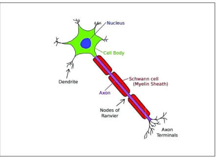
The diversity of connections inside brain link approximately 10 billion nerve cells using a few stereotype electrical signals (Nicholls et al., 1992). At this level of brain organization, it is important to understand the essential aspects of the electrical signalling and chemical interaction within and between neurons. Despite the great variance of neurons morphology, typically neuron consists of dendrites, cell body, axon and axon terminal with specialized function for each part (see Figure 2.4). Dendrites receive inputs and forward the signals towards the cell body where the inputs will be integrated as an information in a form of electrical signals. The signals propagate along the axon towards axon terminals through
shared intracellular volume called the cytoplasm.
Figure 2.4: Schematic view of a typical neuron. ( Figure from http: //commons.wikimedia.org/ )
2.2.1
Local potentials
Central nervous system transmits information by interplay of two types of elec-trical signals called localized potential and action potential. Localized potentials are produced physically by sensory stimulation and neurotransmitters activation (see Section 2.2.3). Transmission of information within neuron occurs through passive propagation of these potentials. Increase distance from the source gives exponential decrement of the localized potentials which may be caused by the membrane resistance and capacitance. Ions flow in axoplasm, the intracellular fluids of axon can be described as a current flow in a poorly insulated cable (Ai-dley, 1989).
Generation of electrical signals results from the movement of ionic currents such as sodium(Na+), potassium(K+), calcium(Ca2+) and chloride(Cl−) across
the cell membrane. Movement of ions are regulated by the selective permeability of the membrane that allows diffusion of selected ions through the ion pumps and
2.2. Neurons 28
ion channels (see Figure 2.5). The distribution of different types of ion channels and ion pumps across the cell membrane determine the resulting membrane ca-pacitance. Most of the ion channels are highly selective permitting specific type of ions to flow across the channels . Similar properties for ion pumps which highly selective to ions in order to restore balance in the ion concentrations inside and outside the cell (Dayan & Abbott, 2005).
Figure 2.5: Ions moving across plasma through (a)The ion channel allows specific type of ions to flow across the channel, and (b)ion pumps maintain balance ions concentrations inside and outside the cell by forcing the ions to move against their concentration gradients when ion pumps break adenosine triphosphate, ATP into energy. (Figure from Elmslie (2001))
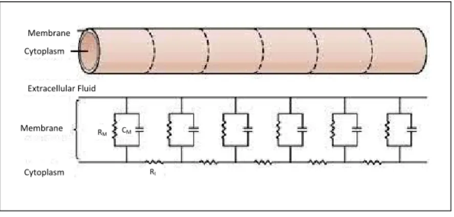
Ionic conductions across neuronal membranes can be represented as voltage and current changes in an equivalent electrical circuit. Considering resistive, ca-pacitive and conductive measures of neuronal membrane, the equivalent circuit model essentially presents the transmission cable properties of neurons (see Fig-ure 2.6) (Ruben, 2001). Propagation of electrical potentials along axon subject to the membrane resistance, RM and intracellular resistance, RI. RM is the
trans-verse resistance of the membrane represents the ion channels. The distance of propagations are subjected to relative differences between RM and RI.
Mem-Membrane Cytoplasm Extracellular Fluid Membrane Cytoplasm RI CM RM M
Figure 2.6: Schematic diagrams of the axon equivalent circuit. RM,membrane resistance;RI,
intracellular resistance;CM, membrane capacitance. (Figure from Kandel et al. (2000))
brane capacitance,CM represents the capacitive properties of neurons membrane
with it capabilities in separating ionic charges between extracellular fluids and cytoplasm.
2.2.2
Action potentials
Movement of ions inward and outward of the neurons is controlled by different internal and external membrane concentrations. This leads to the establishment of electrical potential difference caused by high concentration of potassium (K+)
inside of the membrane and high concentration of Sodium (Na+) outside of the membrane. Equilibrium point is reached if the flow of ions inside and outside of the ions are in balance.
At equilibrium, the cell will have a steady resting condition with excess of negative charges in the intracellular solution compared to extracellular solution (Dayan & Abbott, 2005). The negative potential inside the cell membrane known as resting membrane potential, Vm typically about -65 mV. The magnitudes of
these potentials possibly range between -40mV and -100mV depending on the distribution of electrically charged ions on either side of the membrane and the selective permeability properties of the membrane (Hodgkin & Huxley, 1952). Reduction of membrane resting potential towards 0mV is called depolarization; and increase negativity of membrane potential is called repolarization.
2.2. Neurons 30
Action Potential is automatically excited when membrane potential reaches the threshold level(see Figure 2.7). Generation of action potential is controlled by moving ions across voltage-gated Na+ channel and voltage-gated K+ chan-nel (Ruben, 2001). Rapid membrane depolarization increase the probability of voltage-gated Na+channel being open. After the gate is open Na+ ions enter the cell and influence neighbouring Na+ channels to be activated as well. This
in-crease the membrane permeability towards Na+ions and cause increased amount of Na+ currents entering the cell which eventually decreased internal ions
nega-tivity. Depolarization continues until the number of Na+ions entering the cell are more than the number of K+ ions leaving the cell. In less than one millisecond,
action potential will be generated when depolarization shifts membrane potential from resting state towards threshold level and overshoot the 0mV level (Ruben, 2001).
Figure 2.7: The trace shows depolarization and repolarization of the membrane potential. De-polarization phase occur when Na+ ions enter the cell and decrease the internal ions negativity
until the number of Na+ ions entering the cell are more than the number of K+ ions leaving
the cell. Repolarization phase occur when the membrane permeability towards K+ is increase
and cause a flow of K+ ions leaving the cell. Finally, inactivation of K+ channels shifts the
membrane potential to the initial resting state. (Figure from Freeman, 2005)
Repolarization phase occur when voltage-gated K+ channels are activated simultaneously with inactivation of Na+channel. During this phase, the
intracel-lular potential is decreasing towards resting potential due to increased membrane permeability towards K+. Flow of K+ ions shifts the membrane potential to the
initial resting state. This phase will continue and shifts the membrane poten-tial to undershoot level due to increasing number of K+ ions. Inactivation of K+ channels eventually shifts the membrane potential to the initial resting state
(Ruben, 2001). Refractory period is a short duration where the action potential needs to complete the initial process before initiation of the next action potential. A spike train of action potentials may be produced by prolonged depolarization.
All-or-nothing property of action potential results in automatic response of membrane potential not related to the initial stimulus (local potential) duration and amplitude (Nicholls et al., 1992). Undistorted and rapid propagation of ac-tion potentials along myelinated axon, can be described as informaac-tion conveyed as an electrical conduction within a good insulated cable that is strengthened by regenerative action from the nodes of Ranvier. Voltage-gated ion channels mediate the active signalling process of action potential along the axon without reducing the magnitude of action potential over the distance. Information re-ceived by dendrites are integrated in cell body and transmitted to axon terminal through the propagation of action potentials. Action potentials arriving at axon terminal then initiate the chemical synapse to convey the information towards another neuron.
2.2.3
Synaptic signalling
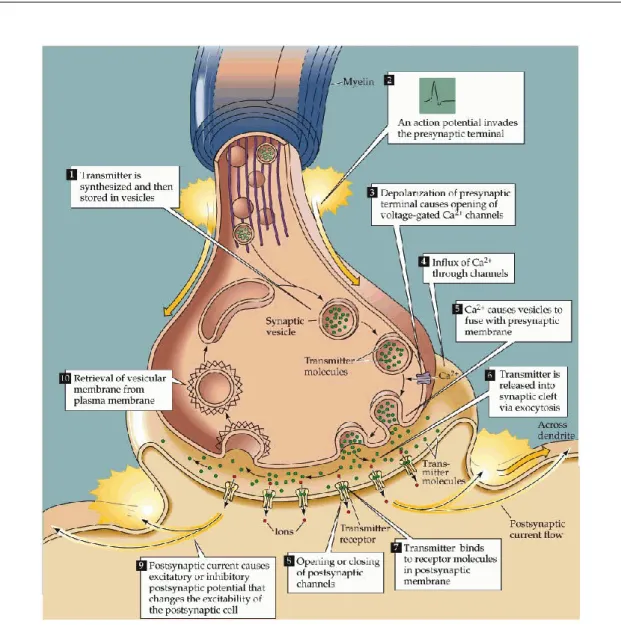
Synaptic signalling is a neuronal communication mechanism that occurs at the molecular level of the brain. Synaptic signalling initiated after arrival of action potential in presynaptic axon terminal followed by opening of voltage gated Ca2+
channels. An influx of Ca2+ ions into the terminal area triggers vesicles contain-ing neurotransmitters to bind with receptors located at presynaptic membrane (see Figure 2.8). The chemical reactions called exocytosis will release neurotrans-mitters that carry the information from presynaptic neuron into the synaptic cleft. There are two main types of neurotransmitters; excitatory neurotransmit-ter (amino acid glutamate) & inhibitory neurotransmitneurotransmit-ter (γ-amino-butyric-acid,
2.2. Neurons 32
GABA). Both types of neurotranmitters will bind with receptors at postsynaptic neurons and form an ions channels (Nicholls et al., 1992; Purves et al., 2008).
Figure 2.8: Synaptic signalling is initiated by electrical signalling followed by chemical event between neurons and finally producing excitatory postsynaptic potential (EPSP) or inhibitory postsynaptic potential (IPSP). (From Purves et al. (2008))
Chemical binding between neurotransmitters and receptors will cause an opening or closing of the ion channels leading to ionic flow trough the membrane thereby produce a conductance change in postsynaptic membrane. Changes in the membrane conductance generate post synaptic current (PSC) which
eventu-ally produces postsynaptic potential (PSP). PSPs determine the probability of action potentials firing in the postsynaptic neurons whereby PSPs that increase the probablities for action potential firing is known as excitatory postsynaptic po-tential (EPSP) and PSPs that reduce the probabilities of action popo-tential firing is known as inhibitory postsynaptic potential (IPSP). Reversal potential is the membrane potential when the net of ionic flows through an ion channel is equal to zero. Generation of EPSPs and IPSPs depends on comparison of reversal poten-tial against action potenpoten-tial threshold (see Figure 2.9). EPSP is generated when reversal potential is more positive than action potential threshold and IPSP is generated when reversal potential is more negative than action potential thresh-old (Purves et al., 2008).
Time (ms)
Figure 2.9: (A) Glutamat-induced EPSP generated when reversal potential,Erev is more
pos-itive than the action potential threshold. (B) GABA-induced IPSP generated when Erev is
more negative than the action potential threshold. (Figure adapted from Purves et al. (2008))
Significant properties of synaptic interaction between neurons can be repre-sented as a basis of the connectivity patterns between neurons. Two examples of neuronal connectivity patterns are synaptic divergence and synaptic conver-gence. Synaptic divergence is a combination of outputs from single axon terminal towards multiple postsynaptic dendrites. Synaptic convergence is a combination of inputs from multiple axon terminals onto a single postsynaptic neuron (Shep-herd, 1990). For example, a single motor neuron may integrate up to 10,000
2.2. Neurons 34
combination of inhibitory and excitatory signals (Kandel et al., 2000). Tempo-ral and spatial distribution in convergence and divergence synapse will give an impact on generation of action potentials at postsynaptic neurons (Williams & Stuart, 2002).
2.2.4
Dendritic processing
Postsynaptic neurons receive excitatory and inhibitory inputs from hundreds of presynaptic neurons through various type of neurotransmitters during chemical synapse (Nicholls et al., 1992). Active dendritic processing generally consists of three main processes; integration, comparison and decision making (London & H¨ausser, 2005). The electrical information from thousands of synapses which converged into a postsynaptic neuron will be integrated by summation of EPSPs and IPSPs. The summed potentials result in depolarization or repolarization of the cell membrane. Sufficient depolarization will change the membrane poten-tial towards the threshold level and eventually trigger the action potenpoten-tial at cell body (Hodgkin & Huxley, 1952). In short, firing of one spike of action potential is a result from integration of EPSPs and IPSPs that reach the threshold level. However, neuronal firing patterns affected by temporal and spatial factor of pas-sive dendritic processing (Euler & Denk, 2001).
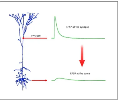
Integration of EPSPs and IPSPs is subject to temporal delay in the trans-mission of electrical potentials caused by the relative distance between synapse location and the cell body. Furthermore, amplitude of PSPs along the dendrites affected by location of voltage-dependent ion channels at the dendritic mem-brane due to possible leakage of ions along the dendrites during transmission which reduce the amplitude of PSPs arriving at the cell body (see Figure 2.10) (Gabbiani & Midtgaard, 2001; Williams & Stuart, 2002). Dendritic processing mechanisms depends on interrelation between dendritic functional properties and morphological structures. Spatial organization of ion channels and neurotrans-mitter receptors in different type of neurons form different mechanism of dendritic
EPSP at the synapse
EPSP at the soma synapse
Figure 2.10: High amplitude of EPSP generated at the synapse location will reduce after an attenuation results in lower amplitude of EPSPs at the soma. ( Figure from Williams & Stuart (2002) )
processing (see Figure 2.11). For example, adjacent location of several synapses may cause local dendrite nonlinear integration of simultaneous inhibitory and ex-citatory potentials and separation between synaptic location will result in parallel linear integration of EPSPs in the cell body. Position of IPSPs along the EPSPs pathways toward the cell body will also reduce the probability of action potential firing (London & H¨ausser, 2005).
Dendrites as a sophisticated computational machine process information from synaptic input by combination of various dendritic mechanisms. Complex dendritic mechanisms however can be modelled to study on single dendrite of sin-gle identified neuron (London & H¨ausser, 2005). Focusing on particular dendrite can help to describe the specific properties of its functional synaptic processing mechanisms. Computational description is necessary to classify the dendritic processing into several processes such as signal filtering, convolution and pattern recognition (London & H¨ausser, 2005). Representation of convergence of synaptic input by the integration between numerous stimulation sites can be used along with axonal processing mechanisms to determine the firing patterns of the neurons for comprehensive illustration of functional effect of single neuron. Established
2.3. Spiking neuron models 36
Local dendrites process
Figure 2.11: Y ellow: Local nonlinear dendritic integration. Green: Longer dendritic pathway significantly attenuate EPSPs signal. Brown: Integration at the cell body followed by com-parison against threshold level before firing an action potential. ( Figure edited from London & H¨ausser (2005) )
functional synaptic map may be associated to functional contributions of the neu-ron on the networks it belongs to (Euler & Denk, 2001).
2.3
Spiking neuron models
Different types of neuron model have been constructed based on different findings in biophysical, anatomical and physiological properties (Dayan & Abbott, 2005). The development of appropriate model considering several main characteristics of neuronal signalling and synaptic transmission is crucial so that essential com-munication principles between neurons can be represented. The behaviour of brain interactions can be mapped out by taking into account the functional con-tribution of neurons in transmitting the information within and between neurons.
Computational and mathematical modelling have long been used to study the complex electrical and chemical interaction of the neurons that lead to the
generation of action potentials. As discussed in the previous section, variable measures of resistance, capacitance and conductance of neuronal membrane exist with respect to the physiological properties of the neuron. Description of such properties by electrical circuits and mathematical models is useful to study the information transmission mechanisms within and between neurons. Three types of neurons modelling approaches briefly described in this section; 1) Hodgkin-Huxley model to describe the functional properties of voltage-dependent mem-brane conductances in firing an action potential by approximating the ion-channel dynamics (Trappenberg, 2010); 2) Integrate-and-fire model to describe functional properties of transmitter-dependent synaptic conductances by approximating the dynamic responses after the integration of presynaptic input (Dayan & Abbott, 2005); 3) Izhikevich model to describe the dynamical properties of various type of neurons; and 4) cortical neural network model for simulation of neuronal network.
2.3.1
Hodgkin-Huxley model
The firing of action potential is initiated by depolarization of membrane poten-tial above the threshold level. Hodgkin-Huxley (HH) model is approximating the mechanism to fire an action potential by taking into account the dynamic properties of moving ions through the voltage-gated ion-channel (Trappenberg, 2010). HH model presents the action potential generation mechanisms by the probability that the channel is active for ion conducting state. The membrane conductance in this model is approximated by the movement of ions across the cell membrane through three different channels. Figure 2.12 shows HH model as an equivalent electric circuit. The total movement of ions,Imresults from the net
movement of a sodium current INa, a potassium current IK, and a small leakage
current IL from non-gated ion channels,
Im=INa+IK+IL. (2.1)
The membrane electrical potentials can be measured by the relation between the ionic currents, Iion with the electrical conductance, gion which controls by the
2.3. Spiking neuron models 38
number of ion channels and the membrane permeability. Such relation is given by the Ohm’s law,
Iion =gion(V −Eion) (2.2)
which corresponds to each ionic component of INa,IK and IL. Eion is the
equilib-rium potential for each channels when no ionic current moving across membrane due to the same concentration inside and outside the cell.
EK K R Na R RL C Iext EL ENa External input
Capacitor Resistance of ion channels
Reversal potentials of ion channels
EK
Figure 2.12: Representation of an equivalent electrical circuit for Hodgkin-Huxley model. This circuit includes a capacitor, two variable resistors to represent voltage-dependant conductances, a static resistor to represent small leakage current and a battery for each channel. (From Trappenberg (2010))
Following to the membrane conductions which are controlled by a set of ion channels, the dynamic properties of the membrane can be determined by the probabilities of activation and inactivations of the ion channels (K+ and Na+).
The probabilities for the voltage dependence ionic channels to open the gate and allow the flow of ions can be described by three dynamic variables; 1) n
indicates the activation of the potassium channels, 2) m indicates the activation of sodium channels and 3) h indicates the inactivation of the sodium channels. The dimensionless variables n, m and h were assumed to vary with time and have a functional dependence on the voltage. The probabilities for ionic flows through potassium channels controlled by four identical events of n, whereby the probabilities for ionic flows through sodium channels controlled by three identical events of m and one event of h. Such probabilities lead to the estimation of the
sodium and potassium conductance,
gNa(V, t) = gNam3h (2.3)
gK(V, t) = gKn4. (2.4)
These variables were selected by Hodgkin and Huxley to fit with the experimental data and can be expressed by the following formula
dn dt = − 1 τn(V) [n−n0(V)] (2.5) dm dt = − 1 τm(V) [m−m0(V)] (2.6) dh dt = − 1 τh(V) [h−h0(V)]. (2.7)
Figure 2.13(A) describe the equilibrium potentials (in mV) for each variables in a function ofV with resting potential is equal to 0 mV. The flip trend ofh0(V) plot
relative to m0(V) distinguish the event of inactivation and activation of sodium
channels. Activation of sodium and potassium channels depicted by the same trend plotted by m0(V) and n0(V), respectively (Dayan & Abbott, 2005). At
resting potential of 0 mV, the probability for sodium channel to be activated is less than 0.1 which is significantly low compared to the event of channels inac-tivation with probability 0.6. In contrast, the probability for potassium channel to be activated is equal to 0.35. This probability values means that the sodium conductance is much smaller than the potassium conductance at equilibrium po-tential of 0 mV.
The time constant τn is the duration for variable, n to approach the
equi-librium value of n0 within a fixed voltage value, V (Gerstner & Kistler, 2002).
The same condition applied for other variables ofm andh. Figure 2.13(B) shows the time constant (in msec) that controls the rate of change for the three vari-ables. At resting potential of 0 mV, τh is the highest (0.85 msec) followed by τn
(0.55msec) and τm with the lowest time constant (0.1 msec). This shows that
2.3. Spiking neuron models 40
response to external stimulation leading to an increase flow of sodium into cell. Sufficient depolarization of the cell membrane will trigger the action potential.
The static conductance from leakage channel remain as constant,
gL=gL. (2.8)
From equation 2.3, 2.4 and 2.8, summation of the three ionic currents can be expressed as (Trappenberg, 2010)
X
ion
Iion =gKn4(V −EK) +gNam3h(V −ENa) +gL(V −EL). (2.9)
HH model equivalent circuit consists of two variable resistors to present voltage dependent ion channels, a constant resistor to represent leakage current, a bat-tery to set the reversal potentials of each ion channel and a parallel capacitor, C to present electric charges stored by the neurons. The changes of the
mem-A. Equilibrium potentials B. Time constants 1000 50 0 50 100 0.2 0.4 0.6 0.8 1 Membrane potential V x0 h n m 0 0 0 1000 50 0 50 100 2 4 6 8 10 Membrane potential V τ0 h n m τ τ τ
Figure 2.13: (A) The equilibrium functions (X0 = probability for activation and inactivation
events ) and (B) time constants ( in unit of msec) for variables n, m and hin HH model. ( Membrane potential in unit of mV ) (Figure from Trappenberg (2010))
brane potential with time according to the behaviour of HH model circuit can be expressed in a first order differential equation,
CdV
dt =−
X
ion
Iion+I(t). (2.10)
External input, I(t) represents an external current which may come from presy-naptic potentials. Inserting equation 2.9 into equation 2.10 and rewriting equa-tion 2.5 to equaequa-tion 2.7 yields the standard differential equaequa-tions of HH model, (Trappenberg, 2010) CdV dt = −gKn 4(V −E K)−gNam3h(V −ENa)−gL(V −EL) +I((2.11)t) τn(V) dn dt = −[n−n0(V)] (2.12) τm(V) dm dt = −[m−m0(V)] (2.13) τh(V) dh dt = −[h−h0(V)]. (2.14)
Figure 2.14 illustrates an example of HH neuron model producing a constant firing rate spike train in response to a constant external current.
Spike train with constant input
0 50 100 50 0 50 100 150 Time [ms] Membrane potential [mV]
Figure 2.14: Membrane potential of HH model shows a constant firing rate spike train initiated by constant external current with sufficient strength. (From Trappenberg (2010))
2.3.2
Integrate-and-Fire neuron model
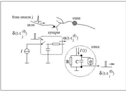
Integrate-and-fire (IF) neuronal model integrates multiple non-interacting presy-naptic inputs written as ana-function with individual synaptic strength value,wj
2.3. Spiking neuron models 42
(See Figure 2.15). a-function is the time course for the postsynaptic current which maybe caused by the chemical interaction of neurotransmitter from presynaptic toward postsynaptic membrane (Trappenberg, 2010). The total input current to
Figure 2.15: Integrate-and-fire neuron model integrates n input channels written as an α -function multiplied by a synaptic strength valuewj. An action potential will be fired when the
total input potential reach a firing threshold. (Edited from Trappenberg (2010)
the postsynaptic neurons expressed by the summation of individual presynaptic events, I(t) = X j X tf j wjα(t−tfj), (2.15)
where tis the postsynaptic firing time and tfj denotes the presynaptic firing time for each synapses, j (Trappenberg, 2010).
Figure 2.16 shows the equivalent electrical circuit for IF neuron model located in the soma. The circuit consists of parallel components of a resistor and a capacitor. The input current, I(t) will split into a resistive current, IR and a
capacitor charging current, IC
I(t) =IR+IC. (2.16)
Referring to membrane potential, v(t) equation 2.16 and can be expressed as
I(t) = v(t)
R +C
dv
dt. (2.17)
Figure 2.16: This figure illustrates a low-pass filter circuit at synapse location to filter presy-naptic currentδ(t−tfj) producing an input current pulse,α(t−tfj). The generated input current pulse will be attenuated to the soma. The IF model equivalent circuit in the soma consists of a reistor, R and a capacitor, C. The capacitor will be charged by the input current, I(t). An output pulse,δ(t−tf
i) is generated at timetfi when the voltage across capacitance increases and
reach the threshold voltage,ϑ. (From Gerstner & Kistler (2002))
the standard equation for IF model,
τm
dv
dt =−v(t) +RI(t). (2.18)
An action potential will be generated at firing time,tf when potential value across
the capacitor reaches the threshold voltage, ϑ
v(tf) = ϑ. (2.19)
With a small delay after the spike generation, the control mechanism will change the membrane state from depolarization into repolarization which will change the membrane potential back to the initial resting potential, vres
lim
δ→0v(t
f+δ) = v
res. (2.20)
Figure 2.17 illustrates an example of IF neuron model producing a spike trains depending on the value of the threshold voltage. A constant interspike interval generated by a stimulation from constant current input with amplitude higher