Range-Based Estimation of Quadratic Variation

(1)

econ

stor

Der Open-Access-Publikationsserver der ZBW – Leibniz-Informationszentrum Wirtschaft

The Open Access Publication Server of the ZBW – Leibniz Information Centre for Economics

Nutzungsbedingungen:

Die ZBW räumt Ihnen als Nutzerin/Nutzer das unentgeltliche, räumlich unbeschränkte und zeitlich auf die Dauer des Schutzrechts beschränkte einfache Recht ein, das ausgewählte Werk im Rahmen der unter

→ http://www.econstor.eu/dspace/Nutzungsbedingungen nachzulesenden vollständigen Nutzungsbedingungen zu vervielfältigen, mit denen die Nutzerin/der Nutzer sich durch die erste Nutzung einverstanden erklärt.

Terms of use:

The ZBW grants you, the user, the non-exclusive right to use the selected work free of charge, territorially unrestricted and within the time limit of the term of the property rights according to the terms specified at

→ http://www.econstor.eu/dspace/Nutzungsbedingungen By the first use of the selected work the user agrees and declares to comply with these terms of use.

zbw

Leibniz-Informationszentrum Wirtschaft

Christensen, Kim; Podolskij, Mark

Working Paper

Range-Based Estimation of Quadratic

Variation

Technical Report / Universität Dortmund, SFB 475 Komplexitätsreduktion in Multivariaten Datenstrukturen, No. 2006,37

Provided in cooperation with: Technische Universität Dortmund

Suggested citation: Christensen, Kim; Podolskij, Mark (2006) : Range-Based Estimation of Quadratic Variation, Technical Report / Universität Dortmund, SFB 475 Komplexitätsreduktion in Multivariaten Datenstrukturen, No. 2006,37, http://hdl.handle.net/10419/22681

(2)

Kim Christensen

†

_{Mark Podolskij}

‡

This Print/Draft: June 29, 2006

Abstract

This paper proposes using realized range-based estimators to draw inference about the quadratic variation of jump-diffusion processes. We also construct a range-based test of the hypothesis that an asset price has a continuous sample path. Simulated data shows that our approach is efficient, the test is well-sized and more powerful than a return-based t-statistic for sampling frequencies normally used in empirical work. Applied to equity data, we show that the intensity of the jump process is not as high as previously reported.

JEL Classification: C10; C22; C80.

Keywords: Bipower Variation; Finite-Activity Counting Processes; Jump Detection; Quadratic

Variation; Range-Based Bipower Variation; Semimartingale Theory.

∗_{Previous versions of this paper were titled "Asymptotic Theory for Range-Based Estimation of Quadratic Variation}

of Discontinuous Semimartingales." The draft was prepared, while Kim Christensen visited University of California, San Diego (UCSD), whose hospitality is gratefully acknowledged. We thank Allan Timmermann, Asger Lunde, Holger Dette, Neil Shephard, Roel Oomen, Rossen Valkanov as well as conference and seminar participants at the 2006 CIREQ conference on "Realized Volatility" in Montréal, Canada, the ESF workshop on "High Frequency Econometrics and the Analysis of Foreign Exchange Markets" at Warwick Business School, United Kingdom, the "International Conference on High Frequency Finance" in Konstanz, Germany, the "Statistical Methods for Dynamical Stochastic Models" conference in Mainz, Germany, the "Stochastics in Science, In Honor of Ole Barndorff-Nielsen" conference in Guanajuato, Mexico, and at Rady School of Management, UCSD, for insightful comments and suggestions. Mark Podolskij was supported by the Deutsche Forschungsgemeinschaft through SFB 475 "Reduction of Complexity in Multivariate Data Structures" and with funding from the Microstructure of Financial Markets in Europe (MicFinMa) network to sponsor a six-month research visit at Aarhus School of Business. The code for the paper was written in the Ox programming language, due to Doornik (2002). The usual disclaimer applies.

†_{Aarhus School of Business, Dept. of Marketing and Statistics, Fuglesangs Allé 4, 8210 Aarhus V, Denmark. Phone:}

(+45) 89 48 63 74, fax: (+45) 86 15 37 92, e-mail: [email protected].

‡_{Ruhr University of Bochum, Dept. of Probability and Statistics, Universitätstrasse 150, 44801 Bochum, Germany.}

(3)

1. Introduction

Modern financial econometrics has largely been developed from the presumption that return-generating processes have continuous sample paths. The workhorse of both applied and theoretical papers is the continuous time stochastic volatility model. These models, however, are contrasted by the many abrupt changes found in empirical data, and a series of recent papers has therefore estimated jump-diffusion processes and/or proposed jump detection tests using i) low-frequency data (e.g., Aït-Sahalia (2002), Andersen, Benzoni & Lund (2002), Pan (2002), Chernov, Gallant, Ghysels & Tauchen (2003), Eraker, Johannes & Polson (2003), Johannes (2004)), or ii) high-frequency data (e.g., Barndorff-Nielsen & Shephard (2004, 2006), henceforth BN-S, Huang & Tauchen (2005), Jiang & Oomen (2005), Andersen, Bollerslev & Diebold (2006)).

Information in high-frequency data, in particular, has provided strong support for jumps in asset prices. The jump component appears to account for a significant proportion of quadratic variation. An asymptotic distribution theory for the preferred test was derived in BN-S (2006), which is based on the ratio of realized variance and bipower variation, suitably normalized. In the presence of microstructure noise, these return-based statistics are often sampled at a moderate frequency to reduce the impact of the noise (e.g., sampling 5-minute returns). This principle, of course, entails a loss of information and much research has been devoted to develop estimators that are more robust to microstructure noise (e.g., Zhang, Mykland & Aït-Sahalia (2004) or Barndorff-Nielsen, Hansen, Lunde & Shephard (2006), among others).

In this paper, we propose a framework using realized range-based estimators to draw inference about the quadratic variation, and we construct a new non-parametric test for jump detection. The motivation for using the range is that intraday range-based estimation of integrated variance is very efficient (see, e.g., Parkinson (1980), Christensen & Podolskij (2006) or Dijk & Martens (2006)). By replacing returns with ranges, we can extract most of the information contained in the data not used by a sparsely sampled realized variance and bipower variation, but without inducing more microstructure noise or relying on complicated corrections to reduce its impact. Hence, we would expect that range-based inference about the jump component is powerful. The properties of the high-low has, however, been neglected in the context of jump-diffusion processes.

Our paper makes several contributions. First, we extend the asymptotic results on the realized range-based variance in Christensen & Podolskij (2006) to cover the jump-diffusion setting. It turns out that this estimator is inconsistent for the quadratic variation of these processes. Second, we introduce range-based bipower variation, derive its probability limit, and asymptotic distribution under the null of a continuous sample path. Third, we use based bipower variation to modify the realized

(4)

range-based variance and restore consistency for the quadratic variation. Fourth, we develop a range-range-based test of the hypothesis of no jump component.

The paper proceeds as follows. In section 2, we set notation and invoke a standard arbitrage-free continuous time semimartingale framework. We review the theory of realized variance within jump-diffusion models and then switch to realized range-based variance. In section 3, we conduct a Monte Carlo study to inspect the finite sample properties of range-based bipower variation and the new jump detection test. In section 4, we progress with some empirical results using high-frequency data from New York Stock Exchange (NYSE). In section 5, we conclude and offer directions for future research. An appendix contains the derivations of our results.

2. A Jump-Diffusion Semimartingale

In this section, we propose a non-parametric method based on the price range for consistently estimating the components of quadratic variation. Moreover, we introduce a new test for drawing inference about the jump part. The theory is developed for a univariate log-price, sayp= (pt)t≥0, defined on a filtered

probability space¡Ω,F,(Ft)_t_≥₀,P ¢

. pevolves in continuous time and is adapted to the filtration(Ft)_t_≥₀,

i.e. a collection ofσ-fields withFu⊆ Ft⊆ F for allu≤t <∞.

Throughout the paper, we assume thatpis a member of the class of jump-diffusion semimartingales that satisfy the generic representation:1

pt=p0+ Z t 0 µudu+ Z t 0 σudWu+ Nt X i=1 Ji, (2.1)

where µ= (µt)t≥0 is locally bounded and predictable, σ= (σt)t≥0 is càdlàg,W = (Wt)t≥0 a standard

Brownian motion, N = (Nt)t≥0 a finite-activity simple counting process, and J = {Ji}i=1,...,Nt is a

sequence of non-zero random variables.2 _{Equation (}_2.1)_with_N _{= 0}_{is called a Brownian semimartingale}

and we writep∈BSM to reflect this in the following.

We assume that high-frequency data are available through[0, t], which is the sampling period and is thought of as being a trading day. At sampling timesti−1 andti, such that0≤ti−1≤ti ≤t, we define

the intraday return ofpover[ti−1, ti]by:

rti,∆i =pti−pti−1, (2.2)

where∆i=ti−ti−1.

1_{Asset prices must be semimartingales under rather weak conditions (e.g., Back (1991)).}

2_{A simple counting process,}_N_{, is of finite-activity provided that}_N

t<∞fort≥0, almost surely. In this paper, we

do not explore infinite-activity processes, although these models have been studied in the context of realized multipower

(5)

With this notation, we can introduce the object of interest; the quadratic variation. The theory of stochastic integration states that this process exists for all semimartingales. Its relevance to financial economics is stressed in several papers (e.g., Andersen, Bollerslev & Diebold (2002)). The definition of quadratic variation is given by:

hpi_t=p-lim n→∞ n X i=1 r2 ti,∆i, (2.3)

for any sequence of partitions0 =t0< t1< . . . < tn=tsuch thatmax1≤i≤n{∆i} →0asn→ ∞(e.g.,

Protter (2004, pp. 66-77)). In our setting,hpi_treduces to:

hpi_t= Z _t 0 σ2udu+ Nt X i=1 Ji2, (2.4)

the integrated variance and squared jumps.

The econometric problem is thathpi_tis latent. We will estimatehpi_t, its two components and test H0 :p∈BSM against Ha :p /∈ BSM from discrete high-frequency data. The basis for our analysis

is an equidistant gridti =i/mn,i = 0,1, . . . ,[mnt], where n is the sampling frequency and [x] is the

integer part ofx.3 _{We then construct intraday returns and ranges:}

ri∆,∆=pi/n−p(i−1)/n, (2.5)

spi∆,∆,m= max{pt−ps}

(i−1)/n≤s,t≤i/n

, (2.6)

fori = 1, . . . ,[nt]. Below, we also use the range of a standard Brownian motion, which is denoted by sWi∆,∆,m, simply replacingpwithW in Equation (2.6).

Our assumptions on the data imply that each interval [(i−1)/n, i/n] contains m+ 1 ultra high-frequency recordings ofpat time pointst(i−1)/n+j/mn,j= 0,1, . . . , m. Of course, the notationspi∆,∆,m

reflects that each range is based on the corresponding m returns. Note that ri∆,∆ is not exhausting

the data, which motivates our approach. This is related to market microstructure noise and will be discussed below. We do not explicitly model the noise in this paper. Instead, we assume that n is chosen such that potential biases from the noise can be ignored.4

3_{In practice, high-frequency data are irregularly spaced and equidistant prices are imputed from the observed ones.}

Two approaches are linear interpolation (e.g., Andersen & Bollerslev (1997)) or the previous-tick method suggested by Wasserfallen & Zimmermann (1985). The former has an unfortunate property in connection with quadratic variation, see Hansen & Lunde (2006, Lemma 1).

4_{A short remark about the setup is appropriate. In the appendix, we start by assuming that}_m _{is infinity. In that}

setting, we suppress dependence onmto writespi∆,∆= sup{pt−ps}

(i−1)/n≤s,t≤i/n

, using the same convention forsWi∆,∆. We then

relax this to finitem. Moreover, we only assume that[0, t]is divided into[nt]equidistant subintervals[(i−1)/n, i/n],

i= 1, . . . ,[nt], for simplicity. The asymptotic results for irregular[ti−1, ti]can be derived as in Christensen & Podolskij (2006). Under suitable conditions, we can also allow for varying number of points and positions in the subintervals. Finally,

(6)

2.1. Realized Variance and Bipower Variation

The availability of high-frequency data in financial economics has inspired the development of a powerful toolkit for measuring the variation of asset price processes. Under the heading realized multipower variation, this framework builds on powers of absolute returns over non-overlapping intervals (e.g., BN-S (2007)).

More formally, we define realized multipower variation by setting: M P V(nr1,...,rk),t=n r+/2−1 [nt_X]−k+1 i=1 k Y j=1 1 µrj |r(i+j−1)∆,∆|rj, (2.7)

withk∈N,rj ≥0 for allj,r+= Pk

j=1rj,µrj =E(|φ|

rj₎_{, and}_φ_∼_N₍₀_,₁₎_.5

Equation (2.7)boils down to many econometric estimators for suitable choices of k and the rk’s.

The most popular isrealized variance (k= 1andr1= 2):

RVn t = [nt] X i=1 r2 i∆,∆. (2.8) RVn

t is the sum of squared returns and by definition consistent forhpitof all semimartingales asn→ ∞.

It follows from Equation (2.4)that:

RVn t p → Z t 0 σ2 udu+ Nt X i=1 J2 i. (2.9) RVn

t measures the total variation induced by the diffusive and jump component. BN-S (2004) introduced

(realized) bipower variation that can be used to separate these parts. The estimator was extended in Barndorff-Nielsen, Graversen, Jacod, Podolskij & Shephard (2006) to weaker conditions. The (first-order) bipower variation is defined as (k= 2,rk= 1):

BVn t = 1 µ2 1 [nt_X]−1 i=1 |ri∆,∆||r(i+1)∆,∆|. (2.10)

Then it holds that:

BVn t p → Z t 0 σ2 udu. (2.11)

Intuitively, the boundedness ofN ensures that the probability of jumps in consecutive returns goes to zero asn→ ∞. Thus, fornsufficiently large, all returns with a jump are paired with continuous returns. The latter converges in probability to zero, so the limit is unaffected by the product.

5_{In the simulation study and empirical application, a small sample correction}_n/₍_n₋_k_{+ 1)}_{is applied to the realized}

(7)

2.1.1. A Return-Based Theory for Jump Detection

BN-S (2004) coupled the stochastic convergence in (2.11) with a central limit theorem (CLT) for

(RVn

t , BVtn), computed under the null of a continuous sample path:

√ n      RVn t − Z t 0 σ2 udu BVtn− Z _t 0 σ2udu      d →M N    0, Z t 0 σ4 udu     2 2 2 2 +ν1        , (2.12) where ν1 = ¡ π2_/₄¢₊_π₋₅_'₀_.₆₀₉₁_and Rt

0σ4uduis the integrated quarticity. Note thatRVtn is more

efficient thanBVn

t . Applying the delta-method to the joint asymptotic distribution of(RVtn, BVtn), we

can construct a non-parametric test ofH0as:

√ n(RVn t −BVtn) s ν1 Z t 0 σ4 udu d →N(0,1). (2.13)

The CLT in (2.13)is infeasible, however, because it depends onR₀tσ4

udu. To implement a feasible test,

we replaceR₀tσ4

uduwith a consistent estimator computed directly from the data. In order not to erode

the power of the test, it is important to use an estimator that is robust to the jump component under Ha. One such statistic isquad-power quarticity (k= 4;rk = 1):

QQn t = 1 µ4 1 [nt_X]−3 i=1 |ri∆,∆||r(i+1)∆,∆||r(i+2)∆,∆||r(i+3)∆,∆|. (2.14)

Now, it holds both underH0andHathatQQnt p

→R₀tσ4

uduasn→ ∞. Hence, this allows us to construct

a feasible test: zRVn t ,BVtn,QQnt = √ n(RVn t −BVtn) p ν1QQnt d →N(0,1). (2.15)

The linear t-statistic in Equation (2.15) can be interpreted as a Hausman (1978) test. Under Ha,

RVn t −BVtn

p

→P_i₌₁_,...,N_tJ2

i ≥0, so the test is one-sided and positive outcomes go againstH0.6 Thus,

we reject H0 if zRVn

t ,BVtn,QQnt exceeds some critical value, z1−α, in the right-hand tail of the N(0,1)

(αis the significance level). Simulation studies in Huang & Tauchen (2005) and BN-S (2006), however, show that (2.15)is a poor description for sampling frequencies used in practice. BN-S (2006) suggested a modified ratio-statistic to improve the asymptotic approximation:

zarRVn t ,BVtn,QQnt = √ n(1−BVn t /RVtn) r ν1max n QQn t/(BVtn)2,1/t o →d N(0,1), (2.16)

6_{Recently, Jiang & Oomen (2005) proposed a two-sided swap-variance test that exploits information in the higher-order}

(8)

where the maximum correction is based on the inequality: QQn t (BVn t )2 p → Z _t 0 σ4 udu µZ _t 0 σ2 udu ¶2 ≥1/t, (2.17)

2.2. Realized Range-Based Variance and Bipower Variation

In theory, the efficient return-based estimators exhaust the data, so we should computeRVnm

t , BVtnm

andQQnm

t . It is well-known thatRVtnmis the maximum likelihood estimator of the quadratic variation

in the parametric version of this problem. Notwithstanding this result, RVnm

t is probably the worst

estimator in practice, as microstructure noise corrupts high-frequency data, which leads to bad inference abouthpi_tifnis too high.

There are some non-parametric estimators that are consistent under various assumptions on the noise process (including the case of endogenous noise), e.g., the subsampler of Zhang et al. (2004) or multiscale estimator of Zhang (2004). This is related to the kernel-based framework studied in Barndorff-Nielsen, Hansen, Lunde & Shephard (2006). The sparsely sampledRVn

t is, however, still the most widely used

volatility statistic in empirical work.

In an earlier paper, we proposed an estimator of the integrated variance, which is based on high-frequency price ranges, see Christensen & Podolskij (2006) and also Dijk & Martens (2006) for related work. This estimator is more efficient thanRVn

t , when microstructure noise is not too severe. Intuitively,

a range extracts some of the information about volatility in data interior toRVn

t . Range-based volatility,

of course, has deep roots in finance and traces back to Parkinson (1980), who studied the scaled Brownian motion,pt=σWt.7 Realized range-based varianceis the high-frequency version of his estimator, though

we were able to handle, essentially, all Brownian semimartingales and discretely sampled high-frequency data. A drawback of the analysis was that we excluded the jump component of Equation (2.1). We close that gap here, among other things.

Realized range-based variance is defined as: RRV_b,tn,m= 1 λ2,m [nt] X i=1 s2pi∆,∆,m, (2.18) whereλr,m =E ¡ sr W,m ¢ andsW,m = max 0≤s,t≤m © Wt/m−Ws/m ª

is the range of a Brownian motion based onmequidistant increments over[0,1]. λr,m removes the bias from discrete data and are related to the

work of Garman & Klass (1980) and Rogers & Satchell (1991). Note thatλr,m is not necessarily finite

for allr∈Randm∈N∪ {∞}. Lemma 1 presents a sufficient condition to ensure this property.

7_{Further readings on range-based volatility estimation can be found in, e.g., Feller (1951), Garman & Klass (1980),}

(9)

Lemma 1 Withr >−m, it holds that

λr,m<∞. (2.19)

It is worth pointing out thatλr≡λr,∞ is finite for allr∈Randλr,1 =µr is not. This result follows,

because form= 1 the range equals the absolute return.

Now, we review the asymptotic results developed forRRV_b,tn,mand extend these in a number of ways. To prove a CLT, we impose some regularity conditions on theσprocess:

(V)σis everywhere invertible (V1) and satisfies:

σt=σ0+ Z _t 0 µ0udu+ Z _t 0 σu0dWu+ Z _t 0 vu0dB0u, (V2) whereµ0_{= (}_µ0

t)t≥0,σ0= (σ0t)t≥0,v0= (v0t)t≥0are adapted càdlàg processes withµ0also predictable and

locally bounded, andB0_{= (}_B0

t)t≥0is a Brownian motion independent of W.

Assumption V1 is a rather technical condition required in the proofs, but it is satisfied for almost

all Brownian semimartingales. V2 is sufficient, but not necessary, and could be weakened to include a

jump process inσ.

The next proposition is adapted from Christensen & Podolskij (2006).

Proposition 1 Assume thatp∈BSM. Then, asn→ ∞

RRV_b,tn,m→p

Z _t 0

σ2udu, (2.20)

where the convergence holds locally uniform int and uniformly inm. Moreover, if condition(V) holds

andm→c∈N∪ {∞}: √ n µ RRV_b,tn,m− Z t 0 σ2 udu ¶ d →M N µ 0,ΛR c Z t 0 σ4 udu ¶ , (2.21)

whereM N(·,·)denotes a mixed Gaussian distribution andΛR

c = ¡ λ4,c−λ22,c ¢ /λ2 2,c.

Note that c affects the asymptotic variance of RRV_b,tn,m, and so its efficiency relative to RVn t . If

m→1 as n→ ∞, ΛR

m →2. If m→ ∞ asn → ∞, ΛRm→0.4073(roughly), so RRVb,tn,m is up to five

times more accurate thanRVn

t , which is an extension of Parkinson (1980).

Maintaining the assumption thatp∈BSM, a consistent estimator ofR₀tσ4

uduis given by therealized

range-based quarticity: RRQn,m_t = n λ4,m [nt] X i=1 s4 pi∆,∆,m p → Z _t 0 σ4 udu, (2.22) so √ n µ RRV_b,tn,m− Z t 0 σ2 udu ¶ p ΛR mRRQn,mt d →N(0,1). (2.23)

(10)

With this result, we can construct confidence intervals forR₀tσ2

udu. It will be clear, however, that neither

RRV_t,bn,mnorRRQn,mt are appropriate choices, ifpexhibits discontinuities. 2.2.1. Extension to Jump-Diffusion Processes

To the best of our knowledge, there is no theory for estimating quadratic variation of jump-diffusion processes with the price range. This raises the question of whether the convergence in probability extends to that situation. The answer, unfortunately, is negative. In fact,RRV_b,tn,mis downward biased ifN6= 0 (andm6= 1), as the subscriptb indicates.

Theorem 1 If psatisfies (2.1), then as n→ ∞:

RRV_b,tn,m→p Z t 0 σ2 udu+ 1 λ2,m Nt X i=1 J2 i, (2.24)

where the convergence holds locally uniform int and uniformly inm.

Theorem 1 shows thatRRV_b,tn,mis inconsistent, except for Brownian semimartingales orm= 1. Nonethe-less, the structure of the problem opens the route for a modified intraday high-low statistic that is also consistent for the quadratic variation of the jump component.

Inspired by bipower variation, we might exploit the corollary: BVtn+λ2,m

³

RRV_b,tn,m−BVtn ´ _p

→ hpi_t. (2.25)

This defies the nature of our approach, however, so we opt for other ways of correcting RRV_b,tn,m. In particular, we introduce the idea of (realized)range-based bipower variation.

Definition 1 Range-based bipower variation with parameter (r, s)∈R2

+ is defined as: RBV₍n,m_r,s₎_,t=n(r+s)/2−1 1 λr,m 1 λs,m [nt_X]−1 i=1 srpi∆,∆,ms s p(i+1)∆,∆,m, (2.26)

Remark 1 In the definition,(i+ 1)may be replaced with(i+q), for any finite positive integerq. Such

"staggering" has been suggested forBVn

t in Andersen et al. (2006) and BN-S (2006). Moreover, Huang

& Tauchen (2005) show that extra lagging can alleviate the impact of microstructure noise by breaking the serial correlation in returns.

RBV₍n,m_r,s₎_,t is composed of range-based cross-terms raised to the powers(r, s)and constitutes a direct analogue to the general definition of bipower variation from BN-S (2004). The parameter setsn(r+s)/2−1_,

(11)

Theorem 2 If p∈BSM, then asn→ ∞

RBV₍n,m_r,s₎_,t→p

Z _t 0

|σu|r+sdu, (2.27)

where the convergence holds locally uniform int and uniformly inm.

Corollary 1 Setr= 0:

RP V₍n,m_s₎_,t →p

Z t 0

|σu|sdu, (2.28)

with the conventionRP V₍n,m_s₎_,t ≡RBV₍₀n,m_,s₎_,t. This estimator is called realized range-based power variation

with parameter s∈R+.

Theorem 2 implies that forr∈(0,2)

RBV₍n,m_r,₂₋_r₎_,t→p

Z _t 0

σu2du, (2.29)

so RBV₍n,m_r,₂₋_r₎_,t provides an alternative way of drawing inference about R₀tσ2

udu. Moreover, it will be

shown below thatRBV₍n,m_r,₂₋_r₎_,tcontinues to estimateR₀tσ2

uduunderHa.

In this paper, we mainly focus on the first-order range-based bipower variation, defined asRBV₍₁n,m_,₁₎_,t≡

RBV_tn,m. Obviously: RBVtn,m p → Z _t 0 σu2du. (2.30)

This subsection is closed by introducing a new range-based estimator that is consistent forhpi_t of the jump-diffusion semimartingale in (2.1):

RRV_tn,m≡λ2,mRRVb,tn,m+ (1−λ2,m)RBVtn,m p

→ hpi_t, (2.31)

i.e. we combine RRV_b,tn,m and RBV_tn,m using the weights λ2,m and 1−λ2,m. This estimator is used

below to compare withRVn t .

2.2.2. Asymptotic Distribution Theory

The consistency ofRBV₍n,m_r,s₎_,tdoes not offer any information about the rate of convergence. Moreover, in practice market microstructure noise effectively puts a bound onn(e.g., at the 5-minute frequency) and it is therefore of interest to know more about the sampling errors. Theorem 3 extends the convergence in probability ofRBV₍n,m_r,s₎_,t to a CLT.8

8_{To prove the CLT, we use the concept of stable convergence. A sequence of random variables,}₍_X_n)

n∈N,converges

stably in law with limitX, defined on an extension of(Ω,F,(Ft)t≥0,P), if and only if for everyF-measurable, bounded

random variableY and any bounded, continuous functiong, the convergencelimn→∞E[Y g(Xn)] =E[Y g(X)] holds.

Throughout the paper,Xn→dsXis used to denote stable convergence. Note that it implies weak convergence in distribution

(12)

Theorem 3 Given p∈BSM and(V)are satisfied, then as n→ ∞andm→c∈N∪ {∞} √ n µ RBV₍n,m_r,s₎_,t− Z t 0 |σu|r+sdu ¶ ds → q ΛBr,s c Z t 0 |σu|r+sdBu, (2.32)

whereB = (Bt)_t_≥₀ is a standard Brownian motion, defined on an extension of

¡

Ω,F,(Ft)_t_≥₀,P ¢

, that

is independent from theσ-field F, and

ΛBr,s c = λ2r,cλ2s,c+ 2λr,cλs,cλr+s,c−3λ2r,cλ2s,c λ2 r,cλ2s,c . (2.33)

Remark 2 Note that the rate of convergence is not influenced by m and no assumptions on the ratio

n/mare required.

Remark 3 Suppose thatpt= Rt

0σudWu, where σis independent ofW and bounded away from zero. If

we have slightly more data than the moment condition in Lemma 1 requires (e.g.,r, s >−m+ 1), then

Theorem 2 and 3 allows for negative values of (r, s). In principle, this meansRBV₍n,m_r,s₎_,t can estimate

integrals with negative powers of σ, e.g.,R₀tσ−2

u du. Unfortunately, it does not seem possible for general

processes without further assumptions. Nevertheless, it is an intriguing feature ofRBV₍n,m_r,s₎_,t, as bipower

variation cannot estimate such quantities.

The critical feature of Theorem 3 is that B is independent ofσ. This implies that the limit process in Equation (2.32) has a mixed normal distribution:

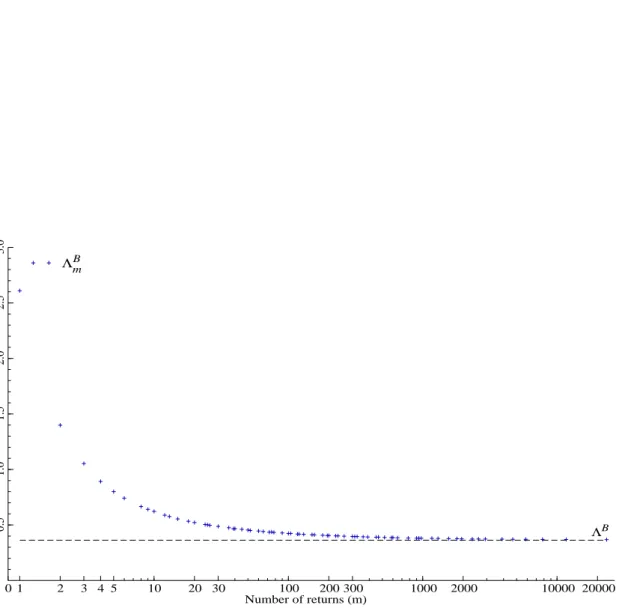
√ n µ RBV₍n,m_r,s₎_,t− Z t 0 |σu|r+sdu ¶ d →M N µ 0,ΛBr,s c Z t 0 |σu|2(r+s)du ¶ . (2.34)

[ INSERT FIGURE 1 ABOUT HERE ]

ΛB m≡Λ

B1,1

m is plotted in Figure 1 for all values ofmthat integer divide 23,400. Asmincreases, there

is less sampling variation, asspi∆,∆,m,i= 1, . . . ,[nt], is based on more increments. A striking result is

that ΛB m → ¡ λ2 2+ 2λ21λ2−3λ41 ¢ /λ4

1 '0.3631 asm → ∞, which is lower than the asymptote ofΛRmof

about0.4073. The break-even point,ΛR

m'ΛBm, is a stunning lowm= 3. This means thatRBVtn,mis

more efficient than RRV_b,tn,m for almost every m under H0, which contradicts both the comparison of

(RVn

t , BVtn)and our intuition. Note thatΛ1B = 2.6091 is the constant appearing in the CLT ofBVtn.

Hence,RBV_tn,mis up to 7.2 times more efficient than BVn

t (asm→ ∞). 2.2.3. A Range-Based Theory for Jump Detection

Now, the univariate convergence in distribution from Proposition 1 and Theorem 3 is extended to the bivariate distribution of³RRV_b,tn,m, RBV_tn,m´. This result is used to propose a new test ofH0.

(13)

Theorem 4 If p∈BSM and(V) holds, then asn→ ∞andm→c∈N∪ {∞} √ n      RRV_b,tn,m− Z t 0 σ2 udu RBV_tn,m− Z t 0 σ2 udu      d →M N    0, Z _t 0 σ4udu     ΛR c ΛRBc ΛRB c ΛBc        , (2.35) with ΛRBc = 2λ3,cλ1,c−2λ2,cλ21,c λ2,cλ21,c . (2.36)

The proof of Theorem 4 is a simple extension of Equation (2.21) and (2.34), so we omit it. By the delta-method, it follows that underH0 (note the subscripting):

√ n(RRV_s tn,m−RBVtn,m) νm Z _t 0 σu4du d →N(0,1), (2.37) whereνm=λ22,m ¡ ΛR m+ ΛBm−2ΛRBm ¢ .

We noticed in Equation (2.31) that RRV_tn,m → hp pi_t. The next theorem shows that, under Ha,

RBVtn,m p

→R₀tσ2

uds. Thus, to implement a feasible range-based test, we need only to substitute Rt

0σu4ds

with a consistent estimator that is robust to jumps. As notedRRQn,m_t is not a suitable choice, because it explodes underHa.

Theorem 5 If p satisfies (2.1), then:

RBV₍n,m_r,s₎_,t→p                    Z t 0 |σu|r+sdu, max (r, s)<2, X∗ t, max (r, s) = 2, ∞, max (r, s)>2, (2.38) whereX∗

t is some stochastic process.

The proof follows the logic of Theorem 5 in BN-S (2004) and is omitted. Note thatRRQn,mt p

→ ∞as n→ ∞ under Ha and RBV₍n,m_r,s₎_,t fails to estimate

Rt

0σu4du, as max (r, s)<2 restricts thatr+s < 4.

It is straightforward, however, to define range-based multipower variation analogous to Equation (2.7). Provided thatmax (r1, . . . , rk)<2, such estimators are robust to the jump component and can estimate

higher-order integrated power variation. We postpone an in-depth treatment of these concepts to later work. In this paper, we only introducerange-based quad-power quarticity:

RQQn,mt = n λ4 1,m [nt_X]−3 i=1

(14)

Now, both underH0 andHa: RQQn,mt p →R₀tσ4 udu, so zRRVn,m t ,RBVtn,m,RQQn,mt = √ n(RRV_p tn,m−RBVtn,m) νmRQQn,mt d →N(0,1). (2.40)

This constitutes our new jump detection test. The intuition is exactly as for realized multipower variation. Based on the above, we would expect a transformation of the t-statistic to improve the size properties in finite samples.9 _{Here we adopt the modified ratio-statistic:}

zar RRVn,m t ,RBVtn,m,RQQn,mt = √ n(1−RBVtn,m/RRVtn,m) r νmmax n RQQn,m_t /(RBV_tn,m)2,1/to d →N(0,1). (2.41)

3. Monte Carlo Simulation

In this section, a Monte Carlo simulation is used to inspect the small sample properties of the asymp-totic results. We untangle the two parts of hpi_t with RBV_tn,m and evaluate the new t-statistic for jump detection, zar

RRVtn,m,RBVtn,m,RQQn,mt . We also compare our test with the return-based t-statistic

zar RVn

t ,BVtn,QQnt. The simulated Brownian semimartingale is given by:

dpu=σudWu

dlnσ2

u=θ(ω−lnσ2u)du+ηdBu,

(3.1)

whereW andB are independent Brownian motions. In this model, the log-variance evolves as a mean reverting Orstein-Uhlenbeck process with parameters(θ, ω, η). We use estimates from Andersen, Benzoni & Lund (2002), setting(θ, ω, η) = (0.032,−0.631,0.374).

To produce a discontinuous sample path forp, we follow BN-S (2006) and allocatejjumps uniformly in each unit of time, j = 1, 2. Hence, the reported power is the conditional probability of rejecting the null, given j jumps. We generate jump sizes by drawing independent N(0, σ2

J) variables and set

σ2

J= 0.05,0.10, . . . ,0.25to uncover the impact on power of varying this parameter.

The remaining settings are: T = 100,000replications of (3.1)are made for allσ2

J. The proportion

of trading each day amounts to 6.5 hours, or 23,400 seconds. This choice reflects the length of regular trading at NYSE, from which our empirical data are collected. We setp0= 0, lnσ02=ω and generate

a realization of (3.1) such that a new observation of p is recorded every 20th second (mn = 1170). Again, this is calibrated to match our real data. RRVtn,m, RBVtn,mand RQQn,mt are then computed

forn= 39,78,390(m= 30,15,3), corresponding to 10-, 5-, and 1-minute sampling.

9_{In unreported simulations, we found that the t-statistic is Equation (}_2.40)_{is highly oversized for sampling frequencies}

(15)

3.1. Simulation Results

In the first row of Figure 2, we plotRBV_tn,mand the integrated variance for 200 iterations of the model with j = 1 and σ2

J = 0.10. The second row shows(RRVtn,m−RBVtn,m) +

against the squared jump, where (x)+ = max (0, x). The maximum correction applied to RRVtn,m−RBVtn,m was suggested by

BN-S (2004) in the context of realized variance, and as RRV_tn,m−RBV_tn,m→p Nt X i=1 J2 i ≥0, (3.2)

we also expect a better finite sample behavior here, although the modified estimator has the disadvantage of being biased.

Asnincreases, both statistics converge to their population counterparts. Atn= 78, they are usually quite accurate, although RBV_tn,m has a larger RMSE relative to (RRV_tn,m−RBV_tn,m)+. According to the CLT, the conditional variance of RBVtn,m is ΛBm

Rt

0σu4dufor Brownian semimartingales. There

is some indication that the errors bounds ofRBV_tn,m increase withσ- most pronounced at n= 390 -but, of course, in our setting jumps are interacting.

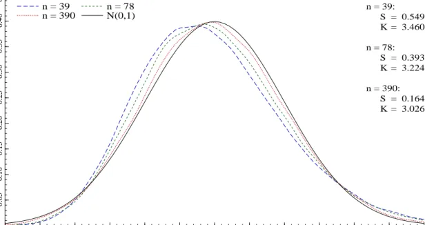
[ INSERT FIGURE 3 ABOUT HERE ] The distribution of zar

RRVtn,m,RBVtn,m,RQQn,mt is plotted in Figure 3 withσ

2

J = 0.00. From Equation

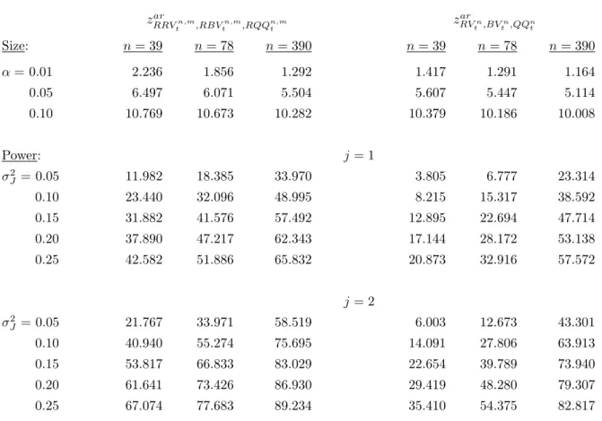
(2.41), the t-statistic then converges to theN(0,1)asn→ ∞, which the kernel-based densities confirm. The approximation is not impressive for moderate n, but the focal point is the right-hand tail, where the rejection region is located. Testing at a nominal level ofα= 0.01with critical valuez1−α= 2.326,

for example, yields actual sizes of 2.236, 1.856 and 1.292 percent, respectively. At α = 0.05 - or z1−α = 1.645 - the type I errors are 6.497, 6.071 and 5.504 percent, in both situations leading to a

modest over-rejection. This finding is consistent with the Monte Carlo studies on zar RVn

t ,BVtn,QQnt in

Huang & Tauchen (2005) and BN-S (2006).

[ INSERT TABLE 1 ABOUT HERE ] The bottom part of Table 1 shows the power ofzar

RRVn,m

t ,RBVtn,m,RQQn,mt across the jump variances

σ2

J = 0.00,0.05, . . . ,0.25with j= 1 andj = 2. The numbers reflect the proportion of t-statistics that

exceededz1−α= 2.326(i.e. no size-correction).

There is a substantial type II error for j= 1 and smallσ2

J, but it diminishes as we depart from the

null. Atσ2

(16)

more quickly forj = 2, reflecting the increase in the jump variation. Consistent with BN-S (2006), we find that power is roughly equal forσ2

J =xandj = 1compared toσJ2 =x/2 andj = 2, showing that

the main constituent affecting the properties of zar RRVn,m

t ,RBVtn,m,RQQn,mt under the alternative is the

variance of the jump process: jσ2

J. As an example, considerj = 2and σJ2 = 0.05; here the fraction of

t-statistics abovez1−α= 2.326is 0.218, 0.340 and 0.585.

Note that the relationship is much weaker at n = 390. Across simulations, there is a pronounced pattern that - keeping jσ2

J fixed - the t-statistic tends to prefer a higher value of σJ2 at the expense of

j for low n, while the opposite holds for largen. Intuitively, at higher sampling frequencies two small breaks in p appear more abrupt, while they are drowned by the variation of the continuous part for infrequent sampling.

As the simulation is designed, mis greater than 1. Hence, the range-based t-statistic ought to be more powerful than the return-based version. We constructRVn

t ,BVtn,QQnt and reportzRVar n

t ,BVtn,QQnt

in the right-hand side of Table 1. In general, the range-based t-statistic is more powerful, in particular, has a much higher probability of detecting small jumps at lower sampling frequencies. Interestingly, though, the size ofzar

RVn

t ,BVtn,QQnt is slightly better than the size ofz ar RRVn,m

t ,RBVtn,m,RQQn,mt .

4. Empirical Application

We illustrate some features of the theory for a component of the Dow Jones Industrial Average as of April 8, 2004. Our exposition is based on Merck (MRK).

High-frequency data for Merck was extracted from the Trade and Quote (TAQ) database for the sample period January 3, 2000 to December 31, 2004. A total of 1,253 trading days. We restrict attention to midquote data from NYSE.10 _{The raw data were filtered for outliers and we discarded}

updates outside the regular trading session from 9:30AMto 4:00PMEST.

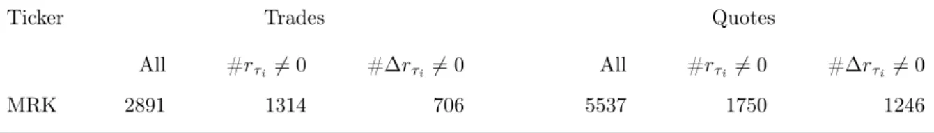
[ INSERT TABLE 2 ABOUT HERE ]

Table 2 reports the amount of tick data. We exclude zero returns - rτi = 0 - and non-zero returns

that are reversals - rτi 6= 0 but ∆rτi = 0 - when computing mn. Here rτi =pτi−pτi−1 and τi is the

arrival time of the ith tick. There is a lot of empirical support for adopting this convention, because counting such returns induce an upward bias inmn- due to transaction price/midquote repetitions and bounces - thus a downward bias in the range-based estimates. Hence, for price changes to affectmn, we require that both rτi 6= 0 and ∆rτi 6= 0. On average, this reduces themn numbers by one-third

(one-half) for the quote (trade) data relative to usingrτi6= 0.

(17)

To account for the irregular spacing of high-frequency data, we usetick-time sampling (e.g., Hansen & Lunde (2006)). We set the sampling timestiat every 15th new quotation (m= 15), which corresponds

to 5-minute sampling on average for our sample and stock. This procedure has the advantage, apart from end effects, of fixing the number of returns in each interval[ti−1, ti]. Tick-time sampling is irregular in

calendar-time, but this is not a problem provided that we also use a tick-time estimator of the conditional variance. Finally, following the recommendation of Huang & Tauchen (2005), we calculate the jump robust estimators by staggering ranges and returns using a "skip-one" approach.

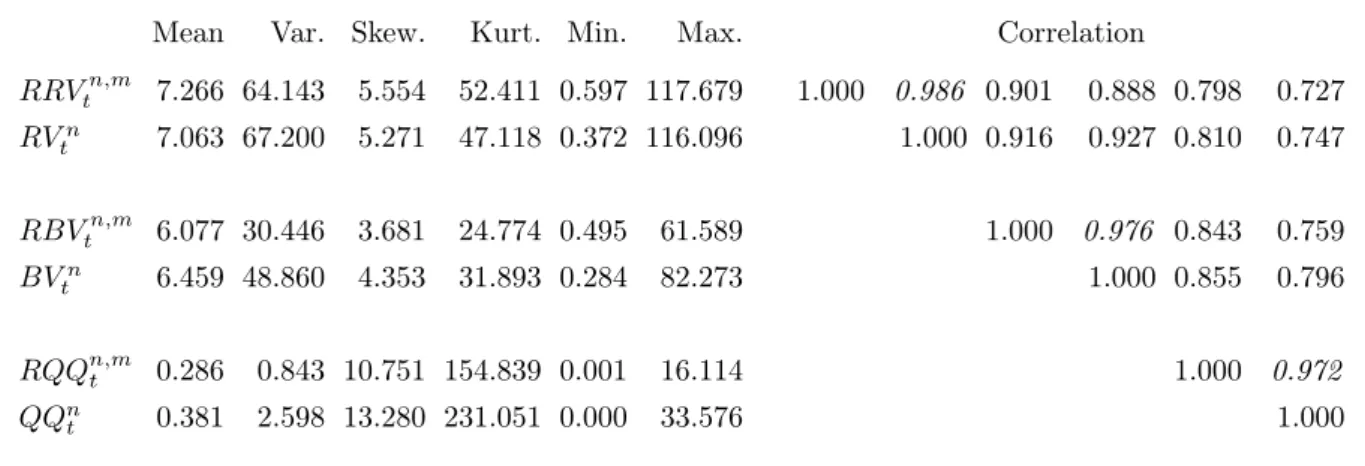
[ INSERT TABLE 3 ABOUT HERE ]

In Table 3, we report some sample statistics of the time series used here. The variance of the realized range-based estimators are smaller compared to the return-based statistics. The reduction is most pronounced for the robust RBV_tn,m and RQQn,m_t . There is a high positive correlation between

(RRVtn,m, RVtn), (RBVtn,m, BVtn) and (RQQn,mt , QQnt), which reflects that they are estimating the

same part of p. Note the large differences in the mean and variance of RQQn,m_t and QQn t. The

maximumQQn

t is twice that ofRQQn,mt . We return to this below.

Figure 4 plotsRRVtn,m (RBVtn,m) against the left (right) y-axis. Both series are reported as

annu-alized standard deviations. The correlation coefficient of the two series is a high 0.901. Moreover, they exhibit a strong own serial dependence, reflecting the volatility clustering in the data. The first five autocorrelations ofRRVtn,m are 0.523, 0.461, 0.383, 0.361 and 0.383, compared to 0.722, 0.644, 0.564,

0.539 and 0.563 forRBV_tn,m. Intuitively,RBV_tn,m is the most persistent process, because it is robust against the (less persistent) jump component. The most important feature of this graph is that some of the spikes appearing inRRV_tn,mare not matched byRBV_tn,m. Here the estimators associate a large proportion ofhpi_tto the jump process, which we now review in more detail.

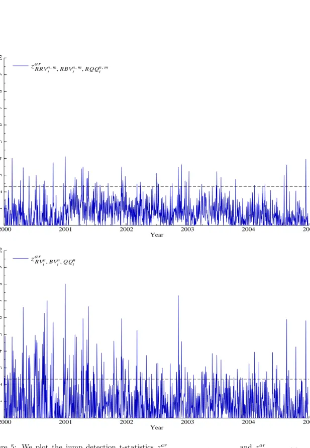
[ INSERT FIGURE 5 ABOUT HERE ] In Figure 5, we plot zar

RRVtn,m,RBVtn,m,RQQn,mt and z ar RVn

t ,BVtn,QQnt. The y-axis is truncated at 0, as

negative outcomes never go againstH0. The horizontal line represents a critical value of z1−α= 2.326,

which is the 0.99 quantile of the N(0,1) density. Figure 5 shows that there is a significant difference betweenzar RRVn,m t ,RBVtn,m,RQQn,mt andz ar RVn t ,BVtn,QQnt.

(18)

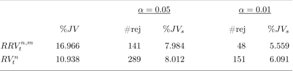
This is underscored in Table 4, where the number of rejections at the 5- and 1% level is shown. We also compute the fraction ofhpi_texplained by the jump process. At the 5% level,zar

RRV_tn,m,RBV_tn,m,RQQn,m_t

rejectsH0 141 times, whilezRVar n

t ,BVtn,QQnt does so 289 times (out of 1,253). Without any jumps at all

in the data, we would expect the t-statistics to reject 63 times. At the 1% level, the numbers are down to 48 and 151 rejections, as opposed to the 13 expected underH0.

Nonetheless, RRVtn,m−RBVtn,m induces a higher proportion of hpit - 16.9% - when all positive,

also insignificant, jump terms are counted. This is because the means ofRRV_tn,m and RBV_tn,m differ more than those ofRVn

t andBVtn. RVtn−BVtn explains 10.9% ofhpit. Taking sampling variation into

account the numbers are aligned, as the range-based t-statistic regards many more of the small jump contributions to be insignificant. At the 1% level,RRVtn,m−RBVtn,m(RVtn−BVtn) accounts for 5.6%

(6.1%) ofhpi_t.

4.1. Estimation of Integrated Quarticity

How much the jump process induces ofhpi_tempirically is an open question. It is unlikely, though, that zar

RVn

t ,BVtn,QQnt picks out so many small jumps z ar RRVn,m

t ,RBVtn,m,RQQn,mt fails to detect. Our simulations

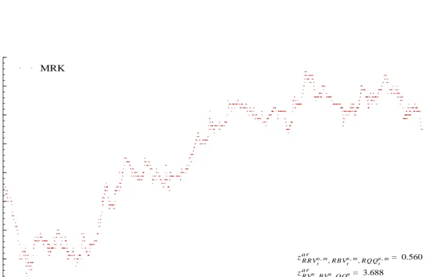
reveal that the latter has higher power to unearth these. To conclude our paper, we therefore inspect this finding a little further. In Figure 6, we draw the data for Thursday, August 24, 2000.

There are several downticks at the beginning of trading, after which the price slopes upward until trading stops. This day has some rapid changes inp, but there is no jump. Stillzar

RVn

t ,BVtn,QQnt = 3.688,

which is a huge rejection. By contrast,zar RRVn,m

t ,RBVtn,m,RQQn,mt = 0.560. Thus, the t-statistics lead to

opposite conclusions about the sample path. We studied Merck’s price at the days in our sample, where zar

RVn

t ,BVtn,QQnt rejected at the 1% level. A majority has slides as in Figure 6 and almost none were

falsely rejected by zar

RRVtn,m,RBVtn,m,RQQn,mt , pointing to more robustness here. This feature, of course,

is relevant to empirical work, because specialists at NYSE are charged with maintaining a smooth price sequence and to avoid large changes between transactions.

We believe that estimation of integrated quarticity is key here. Because of sampling variation,QQn t

is going to deviate somewhat fromR₀tσ4

udurelative toRQQn,mt . Notice from Table 3 that, compared to

RQQn,m_t , the variance of QQn

t is three times larger. Indeed, the asymptotic variance ofQQnt is more

than 9.7 times bigger than that of RQQn,mt (as m → ∞). On days where 1−BVtn/RVtn is small, a

too lowQQn

t can still move the t-statistic into the rejection region, although the lower bound1/tdoes

provide some protection here. We tried to replace QQn

(19)

and, in fact, found that the number of jumps were almost equal.

Recently, Barndorff-Nielsen, Hansen, Lunde & Shephard (2006) proposed an estimator of integrated quarticity that is more robust to microstructure noise, which may enable researchers to further reduce the sampling errors of such return-based estimators by helping to increase the sampling frequency. But realized range-based estimation offers a simple, efficient framework for conducting such inference.

5. Conclusions and Directions for Future Research

This paper proposes using realized range-based estimators to conduct inference about the quadratic variation of asset prices and derives a new test for jump detection. The Monte Carlo study indicates that these estimators are quite efficient at sampling frequencies normally used in applied work, and our empirical results confirm this.

The theory developed here casts new light on the properties of the price range, but there are still several problems left hanging for ongoing and future research. First, the realized range-based estimators were somewhat informally motivated by appealing to the sparse sampling of realized variance caused by microstructure noise. It is not clear how severely microstructure noise affects the range, and we are currently pursuing a paper on this topic. Second, Garman & Klass (1980), among others, construct estimators of a constant diffusion coefficient by combining the daily range and return. Their procedure extends to general semimartingales and intraday data, which suggests that further efficiency gains are waiting. Indeed, other (non-standard) functionals of the sample path could be more informative about the quadratic variation. Third, it will be interesting to connect non-parametric historical volatility measurements using the intraday high-low statistics with model-based forecasting. Fourth, it is also worth considering bootstrap methods to refine the asymptotic normality approximation, as recently suggested by Gonçalves & Meddahi (2005) in the context of realized variance.

(20)

A. Appendix

Note that ast7→σtis càdlàg, all powers ofσare locally integrable with respect to the Lebesgue measure,

so that for anyt ands >0, R₀tσs

udu <∞. Moreover, we can restrict the functions µ,σ, µ0,σ0,v0 and

σ−1 _{to be bounded, without loss of generality (e.g., Barndorff-Nielsen, Graversen, Jacod, Podolskij &}

Shephard (2006)).

A.1. Proof of Lemma 1

The assertion is trivial for r ≥ 0 and is a consequence of Burkholder’s inequality (e.g., Revuz & Yor (1998, pp. 160)). Now, assume−m < r <0and note that:

where φi, i = 1, . . . , m, are IID standard normal random variables. Then, we have the inequality

λr,m≤E ¡ Mr φ ¢ <∞(for−m < r <0). ¥

A.2. Proof of Theorem 1

This theorem is proved by decomposing RRV_b,tn,minto a continuous, jump and mixed part. We adopt the additional notation:

pb t=p0+ Z _t 0 µudu+ Z _t 0 σudWu, pjt=p0+ Nt X i=1 J2 i.

Then, using the finite-activity property ofNt, it follows that:

[nt] X i=1 s2_pj i∆,∆,m p → Nt X i=1 Ji2, [nt] X i=1 s2_pb i∆,∆,m p →λ2,m Z _t 0 σ2udu, 2 [nt] X i=1 spb i∆,∆,mspji∆,∆,m p →0, uniformly inm, where the second convergence is from Christensen & Podolskij (2006). ¥

In the upcoming theorems, we first prove the result withm=∞ and then extend this tom < ∞. To simplify notation, we make the replacements:

g(x) = 1

λr,m

xr_, _h₍_x_{) =} 1

λs,m

xs_,

forx∈R+. We also fix some notation before proceeding. For the processesXn and X, we denote by

Xn p_→_{X, the uniform convergence:}

sup s≤t|X n s −Xs| p →0,

(21)

for allt >0. When Xn _{has the form:} Xn t = [nt] X i=1 ζn i, for an array (ζn i) and Xn p → 0, we say that (ζn

i ) is asymptotically negligible (AN). The constants

appearing below are denoted byC, orCp if they depend on an external parameterp. Finally, to prove

our asymptotic results some technical preliminaries are required.

A.3. Preliminaries I First, we define: βni = √ n|σi−1 n |sWi∆,∆, β 0n i = √ n|σi−1 n |sW(i+1)∆,∆, (A.1) and ρx(f) =E[f(|x|sW)], wheresW = sup{Wt−Ws} 0≤s,t≤1

andf is a real-valued function. Note that ρx(g) =|x|r.

We consider an adapted càdlàg and bounded processν, and the functionf(x) =xp_{, for}_{p >}₀_{. Then,}

we prove a central limit theorem for the quantities Un t = 1 √ n [nt] X i=1 νi−1 n µ f(βn i)−ρσi−1 n (f) ¶ , (A.2) U0n t = 1 √ n [nt] X i=1 µ g(βn i)h(βi0n)−ρσi−1 n (g)ρσi−1 n (h) ¶ . (A.3) Lemma 2 If p∈BSM: Un t ds →Ut= q λ2p−λ2p Z t 0 νuσpudBu, (A.4)

where B = (Bt)t≥0 is a standard Brownian motion, defined on an extension of the filtered probability

space¡Ω,F,(Ft)t≥0,P

¢

and independent from theσ-fieldF.

Lemma 3 If p∈BSM: Ut0n ds → s λ2rλ2s+ 2λrλsλr+s−3λ2rλ2s λ2 rλ2s Z _t 0 |σu|r+sdBu.

Here we prove Lemma 3, leaving Lemma 2 that can be shown with similar techniques. But before doing so, note that the following estimate holds underp∈BSM:

E[|βn

(22)

for allq >0. Lemma 2 and 3 also imply that 1 n [nt] X i=1 νi−1 n f(β n i) p → Z _t 0 νuρσu(f)du, (A.6) and 1 n [nt] X i=1 g(βin)h(β0in) p → Z _t 0 ρσu(g)ρσu(h)du. (A.7) Proof of Lemma 3 We decomposeU0n t into Ut0n= [nt_X]+1 i=2 ζin+γ1n−γ[nnt]+1, with ζn i = 1 √ n µ g¡βn i−1 ¢µ h¡β0n i−1 ¢ −ρσi−2 n (h) ¶ + µ g(βn i)−ρσi−1 n (g) ¶ ρσi−1 n (h) ¶ , γin= 1 √ n µ g(βin)−ρσi−1 n (g) ¶ ρσi−1 n (h). Now, we set ρni−2,i−1(g, h) = Z g ³ σi−1 n x ´ h ³ σi−2 n x ´ δ(dx), where δ(x) = 8 ∞ X j=1 (−1)j+1j2φ(jx),

is the density function ofsW (e.g., Feller (1951)), and we note the identity

Eh|ζn i|2| Fi−1 n i = 1 n µ g¡βn i−1 ¢2µ ρσi−2 n ¡ h2¢₋_ρ2 σi−2 n (h) ¶ +ρ2 σi−1 n (h) µ ρσi−1 n ¡ g2¢₋_ρ2 σi−1 n (g) ¶ + 2g¡βin−1 ¢ ρσi−1 n (h) µ ρni−2,i−1(g, h)−ρσi−2 n (h)ρσi−1 n (g) ¶¶ . Since sup i≤[nt]+1 ¯ ¯_ρn i−2,i−1(gh)−ρσi−2 n (gh)¯¯→p 0, it holds by (A.6) that

[nt_X]+1 i=2 Eh|ζn i|2| Fi−1 n i _p → λ2rλ2s+ 2λrλsλr+s−3λ2rλ2s λ2 rλ2s Z t 0 |σu|2(r+s)du, and sup i≤[nt] |γni| p →0, for anyt. Moreover:

E h ζin| Fi−1 n i = 0.

(23)

AsW =d −W, we also get Ehζn i ³ Wi n−Wi−n1 ´ | Fi−1 n i = 0. Next, assume that N is a bounded martingale on ¡Ω,F,(Ft)t≥0,P

¢

, which is orthogonal to W (i.e. with quadratic covariationhW, Ni_t= 0, almost surely). Asg(βn

i)is a functional ofW times|σi−1 n |

r_{, it}

follows from Clark’s representation theorem (e.g., Karatzas & Shreve (1998, Appendix E)): g(βin)−ρσi−1 n (g) = 1 λr|σ i−1 n | r Z i n i−1 n HundWu,

for some predictable functionHn

u. This also holds forh ¡ β0n i−1 ¢ −ρσi−2 n (h). Hence, E ·³ g(βn i)−ρσi−1 n (g)´ ³Ni n −Ni−n1 ´ | Fi−1 n ¸ = 0, E ·³ h¡β0in−1 ¢ −ρσi−2 n (h) ´ ³ Ni n−Ni−n1 ´ | Fi−1 n ¸ = 0, asN is orthogonal toW. Finally E h ζin ³ Ni n−Ni−n1 ´ | Fi−1 n i = 0. (A.8)

Now, Lemma 3 follows from Theorem IX 7.28 in Jacod & Shiryaev (2002). ¥

A.4. Preliminaries II

We define the process

U(g, h)n_t =√1 n [nt] X i=1 ½ g¡√nspi∆,∆ ¢ h¡√nsp(i+1)∆,∆ ¢ −E h g¡√nspi∆,∆ ¢ h¡√nsp(i+1)∆,∆ ¢ | Fi−1 n i¾ , (A.9)

In this subsection, we show that

U(g, h)n_t −U0n t p →0, (A.10) and, therefore, U(g, h)n_t ds → s λ2rλ2s+ 2λrλsλr+s−3λ2rλ2s λ2 rλ2s Z t 0 |σu|r+sdBu. We begin with: ξn i = √ nspi∆,∆−β n i, ξi0n = √ nsp(i+1)∆,∆−β 0n i , (A.11)

and note that

ξn i ≤ √ n Ã sup| Z t s µudu (i−1)/n≤s,t≤i/n |+ sup| Z t s ³ σu− (i−1)/n≤s,t≤i/n −σi−1 n ´ dWu| ! . A similar inequality holds forξ0n

(24)

Lemma 4 If p∈BSM, it holds that 1 n [nt] X i=1 E£|ξn i|2+|βin+1−βi0n|2 ¤ →0, (A.12) for allt >0. Proof of Lemma 4

The boundedness ofµand Burkholder’s inequality yield

C µ t n+ Z _t 0 E h |σu−−σ[nu] n | 2₊_|_σ u−−σ[nu]+1 n | 2i_du ¶ .

Asσis càdlàg, the last expectation converges to0for almost alluand is bounded by a constant. Thus,

the assertion follows from Lebesgue’s theorem. ¥

To prove the convergence in Equation (A.10), we need the univariate version of Lemma 6.2 and 4.7 from Barndorff-Nielsen, Graversen, Jacod, Podolskij & Shephard (2006). These are reproduced here.

Lemma 5 Let (ζn

i) be an array of random variables satisfying

[nt] X i=1 E h |ζn i|2| Fi−1 n i p →0, (A.13)

for allt. If further eachζn

i isFi+1 n -measurable: [nt] X i=1 ³ ζin−E h ζin| Fi−1 n i´ _p →0.

Lemma 6 Assume that for all q >0

1. f andk are functions on Rof at most polynomial growth.

2. γn

i,γi0n,γ00in areR-valued random variables.

3. The process Zin= 1 + ¯ ¯_γn i ¯ ¯₊_|_γ0n i |+|γi00n|,

(25)

satisfies E[(Zn i)q]≤Cq. If kis continuous and 1 n [nt] X i=1 E h |γ0n i −γi00n|2 i →0, (A.14)

then for allt >0

1 n [nt] X i=1 E h f2₍_γn i) (k(γ0in)−k(γi00n)) 2i →0. (A.15)

Now, we prove (A.10). We define: ζn i = 1 √ n µ g¡√nspi∆,∆ ¢ h¡√nsp(i+1)∆,∆ ¢ −g(βn i)h(βi0n) ¶ , (A.16)

and note thatζn

i isFi+1 n -measurable and U(g, h)n_t −U0n t = [nt] X i=1 ³ ζn i −E h ζn i | Fi−1 n i´ . Appealing to Lemma 5, it is enough to show that:

[nt] X i=1 E h |ζn i |2 i →0. (A.17)

Recall the identity:

√ nspi∆,∆ =β n i +ξni, and, therefore, |ζn i |2≤ C n ³ h2¡√_ns p(i+1)∆,∆ ¢ (g(βn i +ξin)−g(βin))2 +g2₍_βn i) ¡ h¡βn i+1+ξin+1 ¢ −h¡βn i+1 ¢¢2 +g2₍_βn i) ¡ h¡βn i+1 ¢ −h(β0n i ) ¢2´ .