Low-complexity DCD-based sparse recovery algorithms

algorithms

.

White Rose Research Online URL for this paper:

http://eprints.whiterose.ac.uk/117809/

Article:

Zakharov, Yuriy, Nascimento, Vitor, Caiado De Lamare, Rodrigo et al. (1 more author)

(2017) Low-complexity DCD-based sparse recovery algorithms. IEEE Access. 12737 -

12750. ISSN 2169-3536

promoting access to

White Rose research papers

Low-complexity DCD-based sparse recovery

algorithms

Yuriy Zakharov

,

Senior Member

,

IEEE

, V´ıtor Nascimento

,

Senior Member

,

IEEE

,

Rodrigo de Lamare

,

Senior Member

,

IEEE

, and Fernando Goncalves de Almeida Neto

Abstract— Sparse recovery techniques find applications in many areas. Real-time implementation of such techniques has been recently an important area for research. In this paper, we propose computationally efficient techniques based on dichoto-mous coordinate descent (DCD) iterations for recovery of sparse complex-valued signals. We first consider ℓ₂ℓ₁ optimization that can incorporate a priori information on the solution in the form of a weight vector. We propose a DCD-based algorithm for ℓ₂ℓ₁ optimization with a fixed ℓ₁-regularization, and then efficiently incorporate it in reweighting iterations using a warm start at each iteration. We then exploit homotopy by sampling the regularization parameter and arrive at an algorithm that, in each homotopy iteration, performs the ℓ₂ℓ₁ optimization on the current support with a fixed regularization parameter and then updates the support by adding/removing elements. We propose efficient rules for adding and removing the elements. The performance of the homotopy algorithm is further improved with the reweighting. We then propose an algorithm for ℓ₂ℓ₀

optimization that exploits homotopy for the ℓ_{0 regularization;}

it alternates between the least-squares (LS) optimization on the support and the support update, for which we also propose an efficient rule. The algorithm complexity is reduced when DCD iterations with a warm start are used for the LS optimization, and, as most of the DCD operations are additions and bit-shifts, it is especially suited to real time implementation. The proposed algorithms are investigated in channel estimation scenarios and compared with known sparse recovery techniques such as the matching pursuit (MP) and YALL1 algorithms. The numerical examples show that the proposed techniques achieve a mean-squared error smaller than that of the YALL1 algorithm and complexity comparable to that of the MP algorithm.

Index Terms— coordinate descent, DCD, homotopy, sparse recovery

I. INTRODUCTION

Sparse recovery techniques find applications in many areas, including channel estimation [1]–[8], array beamforming [9]– [12], adaptive filtering [13]–[17], and many others that require low-complexity algorithms suitable for real-time implementa-tion. Real-time implementation of sparse recovery techniques, particularly on Field Programmable Gate Arrays (FPGAs), has been recently an important area for research [18]–[25]. There

†_{Department of Electronic Engineering, University of York, UK,} [email protected], [email protected]. ††Dept. of Electronic Systems Eng., University of S˜ao Paulo, Brazil, [email protected]. ‡_{CETUC, PUC-Rio, Rio de Janeiro, Brazil,} [email protected]. ⋆_{Federal Rural University of Pernambuco,} Brazil, [email protected]. The work of Y. V. Zakharov was partly supported by FAPESP-York-2015 grant. The work of V. H. Nascimento was partly supported by CNPq 0306268/2014-0 and FAPESP 2014/50765-6 grants. The work of R. de Lamare was partly supported by FAPESP-York-2015, FAPERJ, and CNPq grants. A part of the material on the ℓ2ℓ1

optimization was presented in the conference Asilomar-2012.

are two families of techniques for finding sparse represen-tations: convex optimization and greedy methods. Generally, greedy techniques have lower complexity and require lower numerical precision [22]. Therefore, when it comes to hard-ware (such as FPGA) implementation, the matching pursuit (MP) algorithm [18], [20], [22] or other greedy algorithms such as CoSaMP [21], [26] or OMP [23], [27] are considered as the most suitable candidates. The MP is a popular greedy technique that possesses especially low complexity and there-fore finds many practical applications [3], [13], [22], [28]– [30]. However, in the accuracy performance, it is inferior to many other techniques.

In the family of convex optimization techniques, there are many algorithms possessing high performance, and recently the YALL1 algorithm implementing the alternating direction method [31], has become popular due to its high accuracy [5], [10]. We will consider the MP complexity and the YALL1 recovery performance as benchmarks when analyzing the algo-rithms that we propose in this paper. The MP, YALL1 as well as our algorithms can deal with complex-valued problems. Often, applications such as channel estimation, beamforming, equalization and many others also require solving complex-valued problems [7], [11], [32]. The family of algorithms capable of dealing with complex-valued problems is scarcer than the family of algorithms for real-valued problems. Impor-tantly, it is not always straightforward to transform real-valued algorithms into complex-valued counterparts [7], [33]–[35]. A complex-valued algorithm can exploit the coupling (common support) of the real and imaginary parts of a signal [35] and potential non circularity of a signal, whereas the real-valued counterpart does not have such a feature. Here we will focus on sparse recovery algorithms for complex-valued problems.

It has been previously recognized that the coordinate descent (CD) search has an inherent property of being low complexity when signals are sparse [36]–[40]. We derive our algorithms applying CD iterations for solvingℓ2ℓ1andℓ2ℓ0optimization

problems. Specifically, we exploit dichotomous CD (DCD) iterations [36] that minimize the use of multiplications, thus resulting in algorithms especially well suited to real-time implementation, e.g. using FPGAs [41]–[44].

In the family of greedy techniques, algorithms based on

ℓ1-homotopy [45] demonstrate high accuracy for recovering

sparse signals and are of lower complexity in comparison with many other techniques [7], [46], [47]. It is important to note that even if the homotopy approach requires solving a sequence of optimization problems for a corresponding sequence of values of a regularization parameter, due to the

iterative nature of the DCD algorithm, if we use the current estimate as the initial condition for the next homotopy iteration (warm initialization), the complexity is in fact reduced, since only a few updates are necessary at each homotopy iteration. We will be using this approach to derive our algorithms.

A prioriinformation on the support of sparse signals can

sig-nificantly improve the algorithm performance. In the extreme case, when the support is perfectly known, the performance of the oracle algorithm is achieved. We will use the oracle

performance as another benchmark for comparison with the performance of the proposed algorithms. However, such a knowledge of the support is most often unavailable. There have previously been proposed techniques for estimating and further refining the information on the support in a set of reweightening iterations and incorporating these estimates in the cost function [48]–[51]. We will exploit this idea to improve the recovery performance of the proposed algorithms. In this paper, we first derive DCD-based algorithms for the weighted ℓ1 penalized regression. Theℓ1-DCD algorithm

updates all elements of the unknown vector. As the vector length can be high, the complexity can also be high. The alternative is a greedy-like algorithm that only deals with a relatively small number of elements within the currently identified support. Therefore, we develop a greedy algorithm that is based on homotopy with respect to theℓ1regularization,

and the ℓ1-DCD iterations are used for updating the solution

within the support. We formulate optimal rules for adding and removing elements from the support. The performance of the homotopy algorithm is further improved with the reweighting. Note that after publishing the initial version of the ℓ2ℓ1

homotopy algorithm in the Asilomar conference [52], it was further developed in [53]–[55] for application in radar imaging and in [56] for application in adaptive filtering.

We then propose an algorithm for ℓ2ℓ0 minimization that

exploits homotopy for the ℓ0 regularization (denoted as Hℓ0

direct-LS algorithm). It alternates between the least-squares (LS) optimization on the support and the support update, for which we also propose efficient rules. We then apply the DCD iterations to solve the sequence of LS problems and arrive at a computationally efficient (Hℓ0-DCD) algorithm.

The paper is organized as follows. Section II describes the signal model. In Section III, we derive the ℓ1-DCD algorithm

forℓ2ℓ1minimization. In Section IV, we present the homotopy

DCD (Hℓ1-DCD) algorithm. Section V presents homotopy

algorithms for ℓ2ℓ0 minimization: Hℓ0 direct-LS and Hℓ0

-DCD algorithms. Section VI contains numerical examples and, finally, Section VII presents conclusions.

Notation: We use capital and small bold fonts to denote

matrices and vectors, respectively; e.g.Ais a matrix andxa vector. Elements of the matrix and vector are denoted asAn,p

and xn, respectively. We use I and Ic to denote a support

(indexes of non-zero elements) and its complement, respec-tively; the cardinality of I is denoted as_|I_|. We also denote: A(q) the qth column of A; AH the Hermitian transpose of A; trace[R] the trace of R;AI the matrix obtained fromA

keeping only columns corresponding to support I; RI,I the

|I|×|I|matrix obtained fromRextracting elements from rows and columns with indexes in the support I; xI the subset of

xthat contains non-zero entries from xcorresponding to the supportI;_ℜ{·}and_ℑ{·}are the real and imaginary parts of a complex number, respectively.

II. SIGNAL MODEL

We consider the linear model

y=Ax+n (1)

whereA_∈CM×N

is the observation matrix,n_∈CM×1 _the

noise vector, y_∈CM×1 _{the observed signal, and x∈C}N×1

the unknown signal. We are especially interested in the case, in whichM < N and all variables in (1) are complex-valued. We also assume that only K < M elements of vector x are non-zero, i.e. the vector x is sparse, and the support (index set of non-zeros) is unknown.

Applications of sparse recovery algorithms differ in the possibility of precomputing the matrix R = AH_{A. If R}

cannot be precomputed, the complexity of algorithms may be dominated by the on-line computation ofRor its submatrices. In other applications, R can be precomputed or updated in real-time with low complexity, e.g. as in adaptive filtering [3], [14], [41], [57], channel estimation [22], beamforming [9]– [11], etc. Here we are interested in applications where R is available.

III. DCDALGORITHM FORℓ2ℓ1OPTIMIZATION WITH FIXED REGULARIZATION

We consider the minimization of theℓ2ℓ1 cost function Jw,τ(x) =

1

2||y−Ax||

2

2+τwT|x| (2)

with a fixed regularization parameterτ, where |x_|is a vector of element-wise magnitudes of entries in x, and w is a weight vector. We now present a direct (non-homotopy) DCD approach for minimization of the cost function in (2), starting with the weight selection and support estimation.

Ifwk = 1for k= 1, . . . , N, this problem is also known as

basis pursuit denoising (BPDN) [58]. We use as benchmark in our simulations anoraclealgorithm, which knows the true location of the nonzero entries. Theoracle algorithm can be obtained by choosingwk= 0forkwithin the support,wk= 1

otherwise, and with τ very large. See other examples of the weight vector in [40], [48], [50].

The weight vector can also be updated in Ns reweighting

iterations and in each iteration, a new problem (2) is solved [7], [49]. We will be using the following updating mechanism. In every reweighting iteration with indexs= 1, . . . , Ns, a weight

supportΓw is identified using hard thresholding:

Γw= n k: _|xk|>(µw)sTwmax n {|xn|} o (3) whereµw∈[0,1]andTw are adjusted parameters. Within the

support Γw, the weight entries are set to a value βs, where

β _∈ [0,1) is an adjusted parameter. In the case of β = 0

andµw = 1, we arrive at the weights in [49]. In the case of

Tw= 1,β = 0andµw= 1/2, we obtain the weights in [59].

The threshold is reduced with every reweighting iteration and (if β > 0) the weights are also reduced. This is reasonable

TABLE I

GENERAL STRUCTURE OF SPARSE RECOVERY ALGORITHMS BASED ON

ℓ2ℓ1OPTIMIZATION WITH REWEIGHTING ITERATIONS

Initialization:c=b=AH_y,x=0,w=1

N,R=AHA

Cu= 0,Ci= 0,Tc=µcmaxk|ck|2 1: fors= 1, . . . , Ns do

2: Solve (2) usingℓ1-DCD or Hℓ1-DCD algorithm

3: For algorithms usingiDCD iterations,

of whichuiterations aresuccessful, compute: Cu←Cu+u,Ci←Ci+i

ifCu≥Nuthenthe algorithm stops (CuandCiare used in the analysis of the algorithm complexity)

4: Update the weight vectorwon the supportΓwusing (3) 5: Debiasing according to (5)

since, in general, the estimation accuracy improves with every reweighting iteration. The term(µw)sprovides an exponential

reduction of the threshold, while βs _{provides an exponential}

reduction of the weights. The parameterµwdefines the rate of

reducing the threshold, whereas the productµwTwdefines the

initial threshold. Note that by choosingβ= 1/2and all initial weights equal to one, the application of the weights does not require multiplications, but only bit-shifts (that are much less costly to implement in hardware).

We are interested in applications where the objective is a low mean squared error (MSE) on the estimated support, e.g. such as estimation of sparse multipath communication channels [1]–[4], [7]. Therefore, after a sparse recovery al-gorithm identifies the support and terminates, a debiasing on the support should be done. The final support I can be the output of the sparse recovery algorithm itself or it can be identified, e.g. using hard thresholding, as a set of elements in the solutionx, satisfying the condition

I=nk : _|xk|> µdmax n {|xn|}

o

(4) where µd ∈ [0,1) is a predefined parameter. Using the finally estimated support I, the debiasing stage computes the minimum MSE (MMSE) estimate of the vector x as the solution to the equation:

(RI,I+νI|I|)xI =AHI y, (5)

whereν =σ2_|I|/trace[R

I,I],σ2is the noise variance andI|I|

is the _|I| × |I| identity matrix.

The general structure of sparse recovery algorithms pro-posed in this paper is shown in Table I. For minimizing the cost function (step 2) at each reweighting iteration s, i

DCD iterations are used among which there are usuccessful

iterations (that is, u iterations in which the solution vector is updated, see [36], [42], [60]; note that the term successful

iterations was introduced in [60]). We set an upper limit Nu

to the total number Cu of successful iterations (considering

all reweighting iterations); the algorithm stops as soon as

Cu=Nu. The parameterTcis used as a threshold to stop the

minimization at step 2; this is checked within the algorithm performed at step 2 (see step 10 in Table II). The total number of DCD iterationsCi and the total number ofsuccessfulDCD

iterationsCu determine the algorithm complexity, as detailed

later in this section.

The function in (2) is convex and we use DCD iterations to minimize it. One difference between our DCD-based al-gorithms and previously proposed CD alal-gorithms [37]–[39], [61] is that we do not optimize the step-size for every CD iteration, but instead we use a set of step-sizes defined by the fixed-point representation of the solution. Thus, our CD search is an inexact line search [62], [63] as opposed to the exact line search in most previously proposed CD algorithms. Although, for a particular iteration, the exact line search achieves a higher reduction of the cost function, with an inexact line search the convergence to the true solution in a sequence of iterations can be even faster. In [41] and [42], this was demonstrated when comparing the exact CD search and the DCD search for solving the LS problem. Importantly, the DCD search allows a large reduction in the number of operations; in many cases, the algorithm complexity is dominated by the complexity of

successful iterations, which typically represent a small part

of all DCD iterations, especially for sparse solutions [36]. Moreover, most of the operations are additions and bit-shifts which, together with the fixed-point representation of the solution, make DCD iterations attractive for implementation on real-time design platforms, such as FPGAs [42].

Consider DCD iterations for minimizing the cost func-tion (2). At every iterafunc-tion, only the p-th element of the solution vector x may be updated as x˜ = x+αep, where

α is a complex-valued scalar and the vector ep has the p-th

element equal to one and the others zero. The update should only be done if the cost function is reduced, i.e. if

∆J=Jw,τ(x+αep)−Jw,τ(x)<0

This can be written in the form

∆J =1

2|α|

2_R

p,p − ℜ{α∗(bp−R(p)Hx)}

+ τ wp(|xp+α| − |xp|) (6)

whereb=AHy. Defining the residual vectorc=b₋Rx, we obtain

∆J = 1

2|α|

2_R

p,p− ℜ{α∗cp}+τ wp(|xp+α| − |xp|) (7)

Starting from x =0 and c= b, the residual vector can be recursively updated at every coordinate descent iteration as c_←c₋αR(p)_{. Ifαis a power-of-two number, the update of}

crequiresM complex additions and no multiplications. Note also that if∆J _≥0, then no update is necessary - we call this low-cost case anunsuccessfuliteration. If∆J <0, an update is necessary - this is a successfuliteration.

When using DCD iterations, it is assumed that elements of the solution vector have a fixed-point representation withMb

bits within an amplitude interval [₋H, H]. The choice of H

may be defined from the maximum magnitude of elements in x. Note that the choice of H is not unique for DCD; in any system with fixed-point representation of signals, one has to decide on the maximum possible amplitude of the signals. It is preferable to choose H as the smallest power-of-two number satisfying H ≥maxq{|ℜ[xq]|,|ℑ[xq]|}. However, the choice

is not very critical; see discussion on the choice ofH in [42]. The DCD iterations start updates from the most significant bits

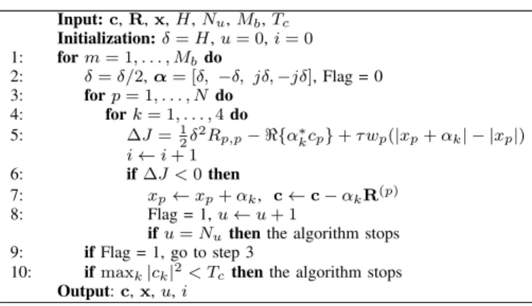
TABLE II ℓ1-DCDALGORITHM Input:c,R,x,H,Nu,Mb,Tc Initialization:δ=H,u= 0,i= 0 1: form= 1, . . . , Mbdo 2: δ=δ/2,α= [δ, −δ, jδ,−jδ], Flag = 0 3: forp= 1, . . . , Ndo 4: fork= 1, . . . ,4do 5: ∆J=1 2δ2Rp,p− ℜ{α∗kcp}+τ wp(|xp+αk| − |xp|) i←i+ 1 6: if∆J <0then 7: xp←xp+αk, c←c−αkR(p) 8: Flag = 1,u←u+ 1

ifu=Nuthenthe algorithm stops 9: ifFlag = 1, go to step 3

10: ifmaxk|ck|2< Tcthenthe algorithm stops

Output:c,x,u,i

of coordinates towards less significant bits. This is controlled by a step-sizeδ >0that starts withδ=H and is reduced as

δ_←δ/2for less significant bits.

In a DCD algorithm for complex-valued problems, for every coordinate, there are four possible directions on the complex plane for updating: 1, ₋1, j and ₋j, where j = √₋1. Consequently, there are four values by which a coordinate can be updated. These are the scalar valuesαk,k= 1, . . . ,4,

defined by these four directions and the step-sizeδas elements of the vector α= [δ, −δ, jδ, −jδ].

There can be different strategies for selecting coordinates for updates. The most often used are cyclic and leading [41] (also called greedy [61]) selections. Leading CD iterations require costly computations for selection of the best coordinate for updating. With cyclic DCD iterations, we do not need to find the minimum of the cost function over all possible updates. The cyclic DCD algorithm for minimizing Jw,τ is shown in Table II. [We have also developed a leading DCD algorithm for minimizing the cost function in (2) that provides an accuracy similar to that of the cyclic DCD algorithm. However, its complexity is somewhat higher than the complexity of the cyclic DCD algorithm. Therefore, here, we only present the cyclic DCD algorithm.] In addition to the parameters of the algorithm described above (Mb and H), we also introduce

the maximum number of successful iterations (i.e. iterations where the solution is updated) Nu and a parameter µc that

defines the threshold Tc for residual magnitudes; µc ∈[0,1)

is a predefined parameter (see Table I). If all the magnitudes are smaller than the threshold, the algorithm stops.

The complexity of the cyclic DCD (we call it ℓ1-DCD)

algorithm in (real-valued) flops is given by

Pℓ1-DCD ≈ 8M N+ 4N+ 11Ci+ 2N Cu

+ 4N Mb+ 2NdebLg (8)

The first and second terms in (8) are for computing c and

Tc at the initialization stage (see Table I); these operations are

multiplications and additions. The term11Ciis the complexity

of Ci tests at steps 5 and 6 in Table II; each computation

involves analysis of one direction on the complex plane for one element, which can be done with 11 real-valued operations, including multiplications, additions, and square-roots (required

to compute the absolute values_|xp|and|xp+αk|). The exact

value ofCi, the number of times the test at step 6 is evaluated,

is difficult to predict; Ci ≥Nu and tends to increase as the

vector length N increases. The term 2N Cu is for updating c in the overall Cu successful (i.e. when ∆J < 0) DCD

iterations (step 7); each update requires only 2N real-valued additions, as multiplications by αk are bit-shift operations.

The next term in (8),4N Mb, is the complexity of computing

square magnitudes_|ck|2 of the residual vector and search for

the maximum to check the termination condition at step 10; this is done for every bitm, thus the factorMb, and involves

multiplications and additions. The debiasing (last term) can be efficiently done by using extra Ndeb DCD iterations at the finally fixed support of cardinality Lg using the previously

found estimate of x as a warm start. The DCD iterations for debiasing are similar to that in Table VI below and only involve additions.

The complexity for theℓ1-DCD algorithm in (8) and other

algorithms below are given in terms of flops. We are using this measure because of the difficulty in estimating complexity for the YALL1 algorithm (which we use here as a benchmark) and the proposed ℓ0 direct-LS algorithm, and because the

true complexity will depend on the particular hardware imple-mentation (e.g., DSPs, which have one-cycle multiplication units, or FPGAs). This way of measuring complexity tends to overestimate the complexity for DCD-based algorithms in FPGA implementations, because DCD avoids multiplications and divisions, which are complicated to implement in hard-ware [64].

Although theℓ1-DCD algorithm demonstrates a high

recov-ery performance and relatively low complexity (as will be seen in Section VI), the complexity can be further reduced. Note that for high N, Ci can be high, and in this case the main

contribution to the ℓ1-DCD complexity are computations at

step 5 in Table II, which are repeated Ci times. Moreover,

these (and only these) computations involve the square-root operation. Although such an operation can be efficiently imple-mented using DCD iterations [65], it is still more complicated for hardware implementation than addition and multiplication. The number of these computations can be significantly reduced if they are only performed on the currently identified support with a size _|I_| that is typically significantly lower than N. This can be done using the homotopy approach as described in the next section.

IV. HOMOTOPYDCDALGORITHM FORℓ2ℓ1 OPTIMIZATION

For minimization ofJw,τ in (2) with further reduced com-plexity, we now use homotopy with respect to the regulariza-tion parameterτ. Ifτis high, the second term in (2) dominates the cost function and forces the cardinality of the presumed support to zero. The strategy is to select the minimum possible value (τmax) for the regularization parameter τ, for which the solution is still all-zeros, and, in homotopy iterations, generate a decreasing sequence of values ofτ using uniform sampling in the log scale; this is similar to the strategy in [40]. We will start withτ =τmax and empty supportI =∅. For every

τ, we will update the support and, on the updated support, minimize the cost functionJw,τ. The algorithm will terminate if τ _≤ τmin, where τmin = µττmax and µτ ∈ [0,1] is a

predefined parameter, or if another termination condition is met. Starting with zero support enables us to work always with a small support, keeping the dimension of the problem at each step low and significantly reducing the complexity.

We need to find rules for adding and removing elements into/from the support.

Proposition 1: Let I be the support at some homotopy iteration and the current solution to the ℓ2ℓ1 minimization be

x. Letb=AHy,R=AHA, andc=b₋Rx. Adding the

t-th element,t∈Ic

, into the support according to the rule

t= arg max

k∈Ic

(_|ck| −τ wk)2

Rk,k

s.t. _|ct|> τ wt (9)

leads to reduction of the cost function (2) for a properly chosen

xt. The value xt= ct Rt,t 1₋τ wt |ct| (10) minimizes the cost function.

Proof. To prove this proposition, we analyze the change

of the cost function due to the update x˜ = x+αet, where

t _∈ Ic_{, i.e. x}

t = 0. The cost function will be changed by

∆J =Jw,τ(x+αet)−Jw,τ(x). We need to check if anα exists that results in∆J <0. We rewrite∆J as

∆J = 1 2|α| 2_R t,t− ℜ{α∗ct}+τ|α|wt = 1 2|α| 2_R t,t− |α|ℜ{e−jarg(α)ct}+τ|α|wt

It is seen that a minimum of ∆J over arg(α) is achieved if

arg(α) =arg(ct)and, in this case, we have

∆J =1

2|α|

2_R

t,t− |α||ct|+τ|α|wt (11)

To find _|α_| minimizing (11), we solve

∂∆J

∂_|α_| =|α|Rt,t− |ct|+τ wt= 0 (12)

and obtain that the minimum of ∆J over _|α_| is achieved at

|α_| = (_|ct| −τ wt)/Rt,t > 0. Thus, ∆J is minimized and

negative if _|ct|> τ wtand α= 1 Rt,t (_|ct| −τ wt)ejarg(ct)= ct Rt,t 1₋τ wt |ct|

In this case, the largest decrement of the cost function Jw,τ is given by ∆J = ₋(1/2)(_|ct| −τ wt)2/Rt,t. Thus, the rule

for adding a new element into the support can be formulated as in (9) and (10).

Note that we are computing the minimum here just to show that adding a new element to the support would lead to a reduction of the cost function. In order to keep computational complexity low, and to keep the fixed-point structure of the solution, we do not actually update the solution using the optimal value of xt in (10); see Table III and the discussion

further below.

This proposition also determines the starting value τmax of

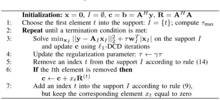
TABLE III Hℓ1-DCDALGORITHM

Initialization:x=0,I=∅,c=b=AH_y,R=AH_A 1: Choose the first elementtinto the support:I={t}; computeτmax

2: Repeatuntil a termination condition is met: 3: SolveminxI||y−AIxI||

2

2+τwIT|xI|on the supportI and updatecusingℓ1-DCD iterations

4: Update the regularization parameter:τ←γτ

5: Remove an indextfrom the supportI according to rule (14) 6: Ifthetth element is removedthen

c←c+xtR(t)

7: Add an indextinto the supportIaccording to rule (9), but keep the corresponding elementxtequal to zero

the regularization parameter τ. If I =_∅, the first element to be added into the support should be the one that maximizes

(_|bt| −τ wt)2/Rt,tover t= 1, . . . , N. Ifwt=const>0 and

Rt,t = 1, we arrive at the rule: t = arg maxk|bk|2. In the

general case,τmax is chosen according to:

τmax= max

k∈Γw |bk|

wk

, where Γw={k:wk >0} (13)

Proposition 2: Let I be the support at some homotopy iteration and the current solution to theℓ2ℓ1 minimization be

x. Let b=AH_{y, R=A}H_{A, and c=b}

−Rx. Removing thet-th element,t_∈I, from the support according to the rule

t= arg min k∈I 1 2|xk| 2_R k,k+ℜ{x∗kck} −τ wk|xk| s.t. 1 2|xt| 2_R t,t+ℜ{x∗tct} −τ wt|xt|<0 (14)

reduces the cost function.

Proof.To prove this proposition, we note that when

remov-ing an element xt from the support, the solution is updated

as x˜ = x₋xtet. The change of the cost function ∆J =

Jw,τ(˜x)−Jw,τ(x)due to this update can be written as

∆J= 1

2|xt|

2_R

t,t+ℜ{x∗tct} −τ wt|xt| (15)

With the condition that ∆J < 0, from (15), the rule (14) follows.

The homotopy DCD (we call it Hℓ1-DCD) algorithm for

solving the ℓ2ℓ1 minimization problem is now presented in

Table III. This algorithm is similar to the algorithm presented in [11] with the difference that the algorithm in [11] does not have a mechanism for removing elements from the support. At each homotopy iteration, the Hℓ1-DCD algorithm first

mini-mizes the cost function on the supportI for the current value of the regularization parameterτ. Then the algorithm updates the support by removing and/or adding elements from/into the support with further reduction of the cost function.

The order of first removing and then adding elements is chosen due to the following reasons. The intention here is to keep the fixed-pointMb-bit format of elements in the solution

vector x. If we first add an element into the support, we have to update the element as defined in (10), and this would change the format as there is no guarantee that the update will provide exactly anMb-bit word. If we do the adding last, then

we do not need to do the assignment (10) and we can keep the element equal to zero since afterward we solve the ℓ2ℓ1

minimization on the support by using DCD iterations and this element will be properly updated within the fixed-point format. When removing an element from the support, we assign to this element a zero-value which is exactly described within the Mb-bit fixed-point format. Moreover, with this order of

updating the support, we avoid the division operations in (10) that are complicated for hardware implementation. Note that computations in (9) do require division by Rk,k. However, if

the dictionaryAis normalized so thatRk,k= 1 or if1/Rk,k

is precomputed, the divisions are avoided.

The regularization parameterτis reduced at each homotopy iteration starting from the maximum valueτmaxfound at step 1 down to a predefined value τmin using the update τ ← γτ. The parameter γ _∈ (0,1) determines how finely we sample the regularization parameter. The closer γ to one, the more accurate the sampling is, but more computations will be required. The algorithm will terminate if τ _≤ τmin, where

τmin =µττmax andµτ ∈[0,1]is a predefined parameter. We

will also set a limitLmaxto the number of homotopy iterations after which the algorithm terminates.

In this algorithm, we have to solve the minimization prob-lem at every homotopy iteration as the parameterτ affects the optimization result. For this purpose we can use the ℓ1-DCD

algorithm as described above with the following modification. The optimization is now performed on the currently identified supportIonly (and not the entire vectorx). This significantly speeds up the computation as the support size is usually smaller than N. However, we keep updating all elements of the residual vector c as they are required for updating the support after the ℓ2ℓ1 optimization step is finished.

The complexity of the Hℓ1-DCD algorithm in terms of

real-valued flops is given by

PHℓ1-DCD = 8M N + 4N+ 11Ci+ 2N Cu

+ 4N L+ 2NdebLg (16)

This is similar to the complexity of the ℓ1-DCD algorithm

given by (8), but there are two differences. The term 4N Lis the complexity of computing square magnitudes _|ck|2 of the

residual vector for checking for termination of DCD iterations; now this is checked for every homotopy iteration, thus the factor L(L is the total number of homotopy iterations). The total number of DCD iterationsCi(with the complexity11Ci)

is now significantly reduced since solving the problem in (2) in each homotopy iteration is performed only on the currently identified support that in general is significantly smaller than the problem size N. The difference in complexity will be demonstrated in Section VI.

V. HOMOTOPY DIRECT-LSALGORITHM AND HOMOTOPY

DCDALGORITHM FORℓ2ℓ0OPTIMIZATION

Consider the minimization of the cost function

Jλ(x) =

1

2||y−Ax||

2

2+λ||x||0 (17)

This is a non-convex problem and its solution is NP-hard. For finding an approximate solution to this problem, we will use homotopy in the regularization parameter λ. If λis high, the second term in (17) dominates the cost function and, at very

highλ, the supportIof the solution must be empty, i.e.,I=_∅. Therefore, it is intuitive to start the homotopy iterations with a highλand zero support. We need to find a minimum value

λmax of the regularization parameter λfor which stillI =_∅. Starting fromλ=λmax in the homotopy iterations,λwill be gradually reduced using the updateλ_←γλ, whereγ_∈[0,1), so that new elements can be added into the support and/or removed from the support. Thus we need to derive rules for updating the support.

For fixed λ and I, the second term of the cost function

Jλ(x)in (17) is also fixed asλ|I|, and minimizing Jλ(x) is

equivalent to minimizing the first term, i.e., solving the LS problem on the supportI. We can alternate between updating the support, which affects the second term in (17), and solving the LS problem on the fixed support, which affects the first term in (17). Adopting this strategy will allow arriving at a low complexity greedy algorithm.

Proposition 3: Let I be the support at some homotopy iteration and the current solution to theℓ2ℓ0 minimization be

x. Letb=AHy,R=AHA, andc=b₋Rx. Adding the

t-th element,t∈Ic

, into the support according to the rule

t= arg max

k∈Ic |ck|2

Rk,k

s.t. _|ct|2>2λRt,t (18)

and assigning to xt the value ct/Rt,t reduces the cost

function (17). The value of the regularization parameter λ

for starting the homotopy iterations is given by λmax =

(1/2) maxk|bk|2/Rk,k.

Proof.(The proof is similar to the proof of Proposition 1)

We notice thatxt= 0and we want to assign to this element a

new value˜xt=α, i.e., obtain a new solutionx˜ =x+αet, so

that the cost function is reduced. Denoting ∆Jλ =Jλ(˜x)−

Jλ(x), we need to check if an α exists that can reduce the

cost function, i.e., make∆Jλ<0. We can write

∆Jλ=

1

2|α|

2_R

t,t− |α|ℜ{e−jarg(α)ct}+λ (19)

The minimum of ∆Jλ over arg(α) is achieved at arg(α) =

arg(ct). The value of the minimum is given by

∆Jλ=

1

2|α|

2_R

t,t− |α||ct|+λ (20)

Minimizing (20) over _|α_| we arrive at _|α_|=_|ct|/Rt,t. Thus,

∆Jλ is minimized atα=ct/Rt,tand the minimum is given

by

∆Jλ=−|

ct|2

2Rt,t

+λ (21)

Rule (18) follows from the greedy strategy of adding to the support only the entry for which the cost reduction is biggest.

This is not the optimal way of finding an element to be added into the support, however it is simple and efficient as shown below.

This rule also determines the starting value ofλ. At the start of the homotopy iterations, the support is empty, i.e.,I =∅, andx=0. Therefore, the first element to be added intoI is

TABLE IV ℓ0HOMOTOPY ALGORITHM

Initialization:x=0,I=∅, b=AH_{y, R=A}H_A 1: t= arg maxk|bk|2/Rk,k, λ= 0.5|bt|2/Rt,t, I={t} 2: Repeatuntil a termination condition is met:

3: Ifthe supportI has been updatedthen

4: SolveRIxI=fI, whereRI=AHIAI andfI=AHIy 5: c←b−RIxI

6: Update the regularization parameter:λ←γλ

7: Remove fromIelements satisfying the rule (23) and, for every removed element, updatec←c+xtR(t) and setxt= 0 8: Add intoI elements satisfying the rule (18) and

(in theℓ0 direct-LS algorithm) setxt=ct/Rt,tand update c←c−xtR(t)or (in the Hℓ0-DCD algorithm) setxt= 0

defined as t= arg max k |bk|2 Rk,k and |bt|2= 2λmaxRt,t (22)

Thus, the maximum value of λ at the start of the homotopy iterations is given by λmax = (1/2) maxk|bk|2/Rk,k. The

optimal value of the first added element is xt=bt/Rt,t.

This rule is similar to the rule of adding new elements into the support in the MP and OMP algorithms, except that in these two algorithms the condition _|ct| > 2λRt,t is not

checked, as if it had been assumed that λ = 0. Besides, in the MP and OMP algorithms, elements cannot be removed from the support. We now introduce a rule for removing an element from the support, which can be important to improve performance in some situations.

Proposition 4: Let I be the support at some homotopy iteration and the current solution to the ℓ2ℓ0 minimization be

x. Letb=AH_y,R=AH_{A, andc=b}

−Rx. Removing thet-th element,t_∈I, from the support according to the rule

t= arg min k∈I ₁ 2|xk| 2_R k,k+ℜ{x∗kck} s.t. 1 2|xt| 2_R t,t+ℜ{x∗tct}< λ (23)

reduces the cost function.

Proof.To prove Proposition 4, we notice that when

remov-ing the t-th element xt from the support and making it zero,

the cost function changes by the value

∆Jλ=

1

2|xt|

2_R

t,t+ℜ{x∗tct} −λ (24)

From (24), we obtain that the condition ∆Jλ < 0 and the

highest decrement of the cost function is achieved for the element defined in (23).

Note that when adding and removing elements from the support, several elements can satisfy the conditions in (18) and (23). Thus, several elements can be simultaneously added and/or removed from the support.

The general structure of the proposed algorithm for solving the ℓ2ℓ0 minimization problem is now presented in Table IV.

For comparison purposes, we present two options for solving the least-squares problems that appear in Table IV: recursive matrix inversion, as described in Table V, and DCD iterations, as described in Table VI. As our simulations show, the per-formance of the two algorithms is similar, but the complexity

TABLE V

SOLVING THEk-THLSPROBLEM

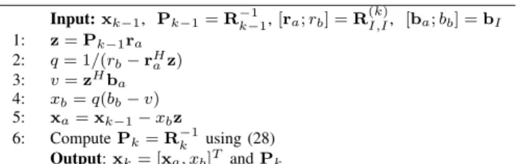
Input:xk−1, Pk−1=R−k−11,[ra;rb] =R(I,Ik), [ba;bb] =bI 1: z=Pk−1ra 2: q= 1/(rb−rHaz) 3: v=zH_b a 4: xb=q(bb−v) 5: xa=xk−1−xbz 6: ComputePk=R−_k1 using (28) Output:xk= [xa, xb]T andPk TABLE VI

DCDITERATIONS FORLSMINIMIZATION

Input:x,c,I,R

Initialization:s= 0,δ=H

1: forform= 1, . . . , Mbdountils=Nu: 2: δ=δ/2,α= [δ, −δ, jδ,−jδ]_{, Flag = 0} 3: forn= 1, . . . ,|I|do:p=I(n) 4: fork= 1, . . . ,4do 5: ifℜ{αkc∗p}> Rp,pδ2/2then 6: xp←xp+αk,c←c−αkR(p) 7: Flag = 1,s←s+ 1 8: ifFlag = 1go tostep 3

of the latter is much smaller.

The complexity of the ℓ0 homotopy algorithm in terms of

real-valued operations is given by

Pℓ2ℓ0 ≈ 8M N+ 4N+PLS+ 4N Lg(Lg+ 1)

+ 12N Lg+ 4L3g (25)

The first and second terms in (25) are the complexity of computing the vector b and selecting the first element into the support at step 1 in Table IV. The termPLS is for solving the LS problems at step 4. The LS problem can be solved using a direct approach that would result in a complexity of

O(L4_{). This can be reduced using the Cholesky factorization}

or conjugate-gradient iterations [33], [66], [67]. A low com-plexity can also be achieved using a recursive inversion of the matrix RI,I; in this case, we have PLS ≈ 4L3g, where

Lg denotes the cardinality of the finally identified support.

Details of the LS recursion are given in Appendix and the recursion is summarized in Table V; here, it is assumed that Rk = RI,I. The term 4N Lg(Lg + 1) is for updating the

residual c at step 5 in Table IV. Adding new elements into the support (step 8) has the complexity12N Lg. The last term

in (25) is the complexity of the debiasing after the support is identified. Removing elements from the support does not involve significant computations and it is not included inPℓ2ℓ0.

Similarly with the Hℓ1-DCD algorithm, the ℓ0 homotopy

algorithms have a combination of stopping criteria. The algo-rithms will terminate if λ≤λmin, where λmin =µλλmax and

µλ∈[0,1]is a predefined parameter. We will also set a limit

Lmax to the number of homotopy iterations after which the algorithm terminates.

For a computationally efficient solution for the sequence of LS problems in theℓ0 homotopy algorithm we can use DCD

iterations as shown in Table VI. The algorithm in Table VI should replace steps 3, 4 and 5 in Table IV. With a limited

number of DCD iterations, one cannot guarantee obtaining the exact LS solution at each homotopy iteration. Therefore, the DCD iterations will be used even when the support is not updated, i.e., step 4 and 5 in Table IV are performed in all homotopy iterations. See more discussion on this matter in [67]. When the DCD iterations start, the vectors x andc are not zeros; here, a warm start of the iterations is used. It is beneficial to use the LS solution found at the previous homotopy iteration as initialization of the DCD algorithm at the current homotopy iteration. As a result, a few DCD iterations may be enough to obtain an accurate LS solution at each homotopy iteration. Elements of x are only updated within the support, whereas all elements ofcare updated. This is necessary for the support update stage of theℓ0 homotopy

to decide on new elements to be added into the support. The algorithm requires a parameter Nu defining the maximum

number of successful DCD iterations, i.e., iterations where the solution is updated. This is necessary for controlling the complexity since the main contribution to the complexity is due to the successfuliterations.

The complexity of the resulting Hl0-DCD algorithm,

per-forming theℓ0homotopy and using DCD iterations for solving

the LS problems, is given by

PHl0-DCD ≈ 8M N+ 4N+ 2CuN+Ci

+ 4N Lg+ 2NdebLg (26)

The first and second terms are for computation of the vector b and selection of the first element in the support at step 1 in Table IV. The term 2CuN is for updating c in the Cu

successful DCD iterations (step 6 in Table VI). The termCi

takes into accountCi(total number of DCD iterations) tests at

step 5 of Table VI to decide if the DCD iteration is successful. Adding new elements into the support (step 8 in Table IV) has a complexity given by the term 4N Lg. Note that, in the

ℓ0-DCD algorithm, we do not set xt = ct/Rt,t to keep the

fixed-point representation of the solution, but instead setxtto

zero; thus, the complexity of this step is reduced comparing to the case of theℓ0direct-LS algorithm. The debiasing (the last

term) is now done by using extra Ndeb DCD iterations at the finally identified support. Note that, in theℓ0-DCD algorithm,

solving the LS problems, which is the most computationally demanding part of the algorithm, is performed using only addition operations. This makes the ℓ0-DCD algorithm very

attractive for hardware design, e.g. on FPGA. VI. NUMERICAL RESULTS

In this section, we compare the MSE performance and complexity of the proposed ℓ1-DCD, Hℓ1-DCD, direct-LSℓ0

-homotopy, and Hℓ0-DCD algorithms with the MP and YALL1

algorithms.

In the YALL1 algorithm, we adjust parameters to guarantee the highest performance and low complexity. The complexity of the YALL1 algorithm is counted based on the number of matrix-vector products, assuming that these are general-type products without using fast transforms, i.e., every such product involves 8M N real-valued operations; when implementing algorithms on FPGAs, it is sometimes preferable to avoid

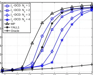
5 10 15 20 25 30 35 40 −40 −35 −30 −25 −20 −15 −10 −5 0 Number of non−zeros MSE (dB) l₁−DCD: N_s = 1 l₁−DCD: N_s = 2 l₁−DCD: N_s = 3 l₁−DCD: N_s = 4 MP YALL1 Oracle

Fig. 1. MSE performance of the ℓ1-DCD algorithm. Parameters of the

scenario: M = 64, N = 256, σ = 0.01. Parameters of the algorithms: Lmax = 80, µd = 0.02, µc = 0.02, µτ = 0.02,γ = 0.9, β = 0.5,

Tw= 1,µw= 0.5,Mb= 8,H= 4,Nu= 4096.

using FFTs, but instead directly compute the products [22]. However, we will also present an example when the FFT can be used. The MP algorithm terminates on achieving the maximum residual magnitude equal to µcmaxk|bk|, where

µc∈[0,1], or a maximum number of greedy iterationsLmax.

For both the YALL1 and MP algorithms, the threshold for debiasing is set to µd = 0.02 [see equation (4)]. On all the plots below, we will also show the MSE performance of an

oracle algorithm that, in each simulation trial, performs the

debiasing on the true support.

We consider simulation scenarios corresponding to channel estimation in communication systems. The channel output is given by y = Ax0+n, where A is a matrix defined by

pilot symbols and x0 is the channel impulse response. The

matrix A is an M ×N circulant matrix generated from an

N×1vector of pilot symbols; for more details on generating the matrixAin channel estimation scenarios see e.g. [1], [4], [7]. The pilot symbols are independent zero-mean Gaussian random numbers. In each simulation trial, a new pilot signal, new channel impulse responsex0, and new realization of noise

are generated. The positions of the K non-zero elements in x0 are chosen randomly, the non-zero elements are generated

as independent complex-valued Gaussian zero-mean random numbers of unit variance and thenx0is normalized to energy K. The noise vector n contains complex-valued random Gaussian entries of varianceσ2_{. For a fixed K, we run1000}

simulation trials and average the MSE MSE=||x−x0||

2 2 ||x0||22

obtained in the trials, where x0 is the true vector (channel

impulse response to be estimated) and xis its estimate. In the proposed DCD-based algorithms, for debiasing, we use extraNdeb= 256DCD iterations.

We consider the case ofN= 256 andM = 64. Fig. 1 and Fig. 2 show the MSE performance and complexity of the

pro-5 10 15 20 25 30 35 40 105 106 107 Number of non−zeros Operations l 1−DCD: Ns = 1 l 1−DCD: Ns = 2 l₁−DCD: N_s = 3 l₁−DCD: N_s = 4 MP YALL1

Fig. 2. Complexity of theℓ1-DCD algorithm. Parameters of the scenario:

M = 64,N = 256,σ= 0.01. Parameters of the algorithms:Lmax = 80,

µd= 0.02,µc= 0.02,µτ= 0.02,γ= 0.9,β= 0.5,Tw= 1,µw= 0.5, Mb= 8,H= 4,Nu= 4096. 5 10 15 20 25 30 35 40 −40 −35 −30 −25 −20 −15 −10 −5 0 Number of non−zeros MSE (dB) Hl 1−DCD: Nu = 1 Hl 1−DCD: Nu = 2 Hl 1−DCD: Nu = 8 Hl 1−DCD: Nu = 32 MP YALL1 Oracle

Fig. 3. MSE performance of the Hℓ1-DCD algorithm. Parameters of the

scenario: M = 64,N = 256,σ = 0.01. Parameters of the algorithms: Lmax= 80,µd= 0.02,µc= 0.02,µτ = 0,γ= 0.9,Ns= 1,Mb= 8,

H= 4.

posed ℓ1-DCD algorithm. When solving the BPDN problem

(i.e., wk = 1 for k = 1, . . . , N, and Ns = 1), the YALL1

algorithm outperforms the ℓ1-DCD algorithm. However, the

reweighting iterations allow significant improvement in the

ℓ1-DCD performance. With one weight update (Ns= 2), the

ℓ1-DCD performance matches the YALL1 performance. With

extra reweighting iterations up to Ns= 4, the performance is

further improved almost reaching its best atNs= 4; additional

iterations do not bring significant improvement. Note that the ℓ1-DCD complexity does not increase considerably with

increasingNs(due to thewarm startof the reweighting

itera-tions) and it is considerably lower than the YALL1 complexity. However, the complexity of sparse recovery can be reduced when using the Hℓ1-DCD algorithm, as shown in Fig. 4.

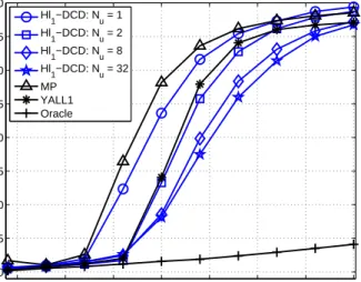
Fig. 3 and Fig. 4 show the MSE performance and com-plexity of the Hℓ1-DCD algorithm without reweighting for

5 10 15 20 25 30 35 40 104 105 106 107 Number of non−zeros Operations Hl 1−DCD: Nu = 1 Hl 1−DCD: Nu = 2 Hl₁−DCD: N_u = 8 Hl₁−DCD: N_u = 32 MP YALL1

Fig. 4. Complexity of the Hℓ1-DCD algorithm. Parameters of the scenario:

M = 64,N = 256,σ= 0.01. Parameters of the algorithms:Lmax= 80,

µd= 0.02,µc= 0.02,µτ= 0,γ= 0.9,Ns= 1,Mb= 8,H= 4. 5 10 15 20 25 30 35 40 104 105 106 Number of non−zeros Operations Hl 1−DCD: Nu = 1 Hl 1−DCD: Nu = 2 Hl₁−DCD: N_u = 8 Hl₁−DCD: N_u = 32 MP YALL1

Fig. 5. Complexity of the Hℓ1-DCD algorithm. Here, it is assumed that

the FFT is used for fast computation of the matrix-vector products in all the algorithms. In the MP and Hℓ1-DCD algorithms, there is one such a product

at the initialization stage. Parameters of the scenario:M = 64,N = 256, σ= 0.01. Parameters of the algorithms:Lmax= 80,µd= 0.02,µc= 0.02,

µτ= 0,γ= 0.9,Ns= 1,Mb= 8,H= 4.

different limitsNuto the number ofsuccessfulDCD iterations.

It is seen that the Hℓ1-DCD algorithm achieves the YALL1

performance with as few asNu= 2successfulDCD iterations

per one homotopy iteration. In this case, the complexity of the Hℓ1-DCD algorithm is close to the MP complexity or even

lower. WithNu>2, the Hℓ1-DCD algorithm outperforms the

YALL1 algorithm and its complexity is significantly lower than the YALL1 complexity. It is interesting to notice that the ℓ1-DCD algorithm (which is a member of the convex

optimization family as all elements of the solution vector are updated) could not achieve the YALL1 performance without the reweighting iterations, whereas the Hℓ1-DCD algorithm

(which belongs to the family of greedy algorithms) can. Fig. 5 shows complexity of the algorithms when the FFT is used for computation of the matrix-vector products. It can be seen

5 10 15 20 25 30 35 40 −40 −35 −30 −25 −20 −15 −10 −5 0 Number of non−zeros MSE (dB) Hl₁−DCD (no remove): N_u = 2 Hl 1−DCD (no remove): Nu = 32 Hl 1−DCD: Nu = 2 Hl₁−DCD: N_u = 32 MP YALL1 Oracle

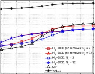
Fig. 6. MSE performance of the Hℓ1-DCD algorithm with and without

the procedure for removal of elements from the support. Parameters of the scenario: M = 64,N = 256,σ = 0.01. Parameters of the algorithms: Lmax= 80,µd= 0.02,µc= 0.02,µτ = 0,γ= 0.9,Ns= 1,Mb= 8, H= 4. 5 10 15 20 25 30 35 40 104 105 106 107 Number of non−zeros Operations Hl 1−DCD (no remove): Nu = 2 Hl 1−DCD (no remove): Nu = 32 Hl₁−DCD: N_u = 2 Hl₁−DCD: N_u = 32 MP YALL1

Fig. 7. Complexity of the Hℓ1-DCD algorithm with and without the

procedure for removal of elements from the support. Parameters of the scenario: M = 64,N = 256,σ = 0.01. Parameters of the algorithms: Lmax= 80,µd= 0.02,µc= 0.02,µτ = 0,γ= 0.9,Ns= 1,Mb= 8,

H= 4.

that the difference in complexity is now smaller, but still the Hℓ1-DCD algorithm is significantly faster than the YALL1

algorithm.

Fig. 6 and Fig. 7 compare two versions of the homotopy al-gorithm. The first one is the Hℓ1-DCD algorithm as described

in Table III, and the other one is the Hℓ1-DCD algorithm,

but without removing elements from the support, i.e., without steps 5 and 6 in Table III. It is seen that, for Nu = 2,

the effect of removing the elements is significant in both the improvement in the MSE performance and reducing the complexity. This can be explained by the fact that, with a small number of DCD iterations, due to inaccurate solving theℓ2ℓ1

problem in every homotopy iteration, there are wrong elements added into the support, which, when removed, improve the

5 10 15 20 25 30 35 40 −40 −35 −30 −25 −20 −15 −10 −5 0 Number of non−zeros MSE (dB) Hl₁−DCD: N_s = 1 Hl₁−DCD: N_s = 2 Hl₁−DCD: N_s = 3 Hl₁−DCD: N_s = 4 MP YALL1 Oracle

Fig. 8. MSE performance of the Hℓ1-DCD algorithm with reweighting

iterations. Parameters of the scenario: M = 64,N = 256, σ = 0.01. Parameters of the algorithms:Lmax= 80,µd= 0.02,µc= 0.02,µτ= 0,

γ= 0.9,β= 0.5,Tw= 1,µw= 0.5,Mb= 8,H= 4,Nu= 8. 5 10 15 20 25 30 35 40 104 105 106 107 Number of non−zeros Operations Hl 1−DCD: Ns = 1 Hl 1−DCD: Ns = 2 Hl₁−DCD: N_s = 3 Hl₁−DCD: N_s = 4 MP YALL1

Fig. 9. Complexity of the Hℓ1-DCD algorithm with reweighting iterations.

Parameters of the scenario:M= 64,N= 256,σ= 0.01. Parameters of the algorithms:Lmax= 80,µd= 0.02,µc= 0.02,µτ = 0,γ= 0.9,β= 0.5,

Tw= 1,µw= 0.5,Mb= 8,H= 4,Nu= 8.

performance. With the largerNu (Nu = 32in this case), the

ℓ2ℓ1problem is accurately solved at every homotopy iterations

and the removal is not that necessary; even if some wrong elements are added into the support, the large number of DCD iterations would drive them to zero and they are removed at the hard thresholding of the debiasing stage.

The reweighting iterations (see Fig. 8 and Fig. 9) result in further improvement of the MSE performance of the Hℓ1-DCD

algorithm and the final performance is close to that achieved by theℓ1-DCD algorithm (compare with Fig. 1). Notice that

with increase inNsbeyondNs= 3, the Hℓ1-DCD MSE curve

departs from the oracle MSE curve. This can be explained by the less reliable support detection with higher Ns as the

threshold for support detection is reduced and thus wrong elements are picked up in the support. Comparing Fig. 9 with

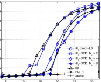
5 10 15 20 25 30 −40 −35 −30 −25 −20 −15 −10 −5 0 Number of non−zeros MSE (dB) Hl 0 direct−LS Hl 0−DCD: Nu = 2 Hl₀−DCD: N_u = 4 Hl₀−DCD: N_u = 8 MP YALL1 Oracle

Fig. 10. MSE performance of theℓ0 direct-LS and Hℓ0-DCD algorithms.

Parameters of the scenario:M= 64,N= 256,σ= 0.01. Parameters of the algorithms:Lmax= 80,µd= 0.02,µc= 0.02,µλ= 0,γ= 0.9,Mb= 8, H= 4. 5 10 15 20 25 30 104 105 106 107 Number of non−zeros Operations Hl 0 direct−LS Hl₀−DCD: N_u = 2 Hl 0−DCD: Nu = 4 Hl₀−DCD: N_u = 8 MP YALL1

Fig. 11. Complexity of theℓ0direct-LS and Hℓ0-DCD algorithms.

Param-eters of the scenario: M = 64,N = 256, σ = 0.01. Parameters of the algorithms:Lmax= 80,µd= 0.02,µc= 0.02,µλ= 0,γ= 0.9,Mb= 8,

H= 4.

Fig. 2, it is seen that the complexity of the Hℓ1-DCD algorithm

is significantly lower than that of theℓ1-DCD algorithm.

Fig. 10 and Fig. 11 show MSE performance and complexity of the Hℓ0 direct-LS and Hℓ0-DCD algorithms. The Hℓ0

direct-LS algorithm shows an MSE performance similar to that of the YALL1 algorithm. The Hℓ0-DCD algorithm matches the

YALL1 performance and the Hℓ0 direct-LS performance with Nu= 8, i.e., with at most 8 DCD iterations per one homotopy

iteration. The complexity of the Hℓ0-DCD algorithm is lower

than complexities of the other proposed algorithms. It is comparable to the MP complexity or even lower. Note that the LS optimization in the Hℓ0-DCD algorithm and debiasing

are multiplication-free. Thus the number of multiplications is only a small part of the whole complexity. E.g., forNu = 8,

only about 20% of operations are multiplications. Thus, this

algorithm is well suited to hardware implementation, e.g. on FPGAs.

VII. CONCLUSIONS

In this paper, we have proposed a family of computationally efficient algorithms for recovery of complex-valued sparse signals. The algorithms are based on solving either the ℓ2ℓ1

or ℓ2ℓ0 optimization problem using dichotomous coordinate

descent (DCD) iterations. We have first derived an algorithm (ℓ1-DCD algorithm) for solving theℓ2ℓ1optimization problem

with a fixedℓ1-regularization term. This algorithm has shown

a high recovery performance and relatively low complexity; specifically, its performance is better and the complexity is lower than that of the YALL1 algorithm. The complexity has been further reduced when combining this algorithm with homotopy with respect to the regularization term. The combined algorithm (Hℓ1-DCD algorithm) has demonstrated a

performance similar to that of theℓ1-DCD algorithm. We have

then derived an algorithm (direct-LS homotopy algorithm) for solving the ℓ2ℓ0 optimization problem using homotopy with

respect to the ℓ0 regularization term. Although the recovery

performance of the algorithm is somewhat inferior to that of the ℓ2ℓ1 based algorithms, its complexity is lower and

comparable to that of the matching pursuit (MP) algorithm. We have then incorporated DCD iterations into the direct-LS

ℓ0homotopy algorithm and arrived at another algorithm (Hℓ0

-DCD algorithm) that has especially low complexity that is comparable or even lower that that of the MP complexity. Moreover, most operations required for implementation of the Hℓ0-DCD algorithm are additions, which makes it very

attractive for real-time implementation, e.g. on FPGAs. APPENDIXI

RECURSIVE SOLUTION OF THE SEQUENCE OFLSPROBLEMS

Let at (k ₋ 1)-th iteration a system of equations Rk−1xk−1 = ba be solved and the solution be xk−1 =

R−_k−1₁ba, where Rk−1 ∈ C(k−1)×(k−1) and xk−1,ba ∈

C(k−1)×1_{. At thek-th iteration, we need to solve an augmented}

systemRkxk =b, where Rk = Rk−1 ra rHa rb and b= ba bb (27) The solution can be found using the formula for inversion of a block matrix as follows:

xk=R−k1b= R−_k−1₁+qzzH ₋qz −qzH _q ba bb (28) wherez=R−_k−1₁ra andq= 1/(rb−rHa z). We represent the

solution in the form:

xk= xa xb (29) Then, noticing thatxk−1=R−k−11ba, we can write:

xa = xk−1+qzzHba−qzbb

Thus, we arrive at the algorithm presented in Table V. Complexity of the technique is mostly defined by steps 1 and 6, each of complexity _O(k2_{). The matrix-vector}

multipli-cation at step 1 involves about8(k₋1)2_{real-valued operations,}

and generating Pk=R−k1 at step 6, taking into account that

the matrix Rk is Hermitian, involves about2(2k+ 1)(k−1)

operations. Complexity of the other steps is O(k). Thus, the complexity of the LS solution update at the k-th iteration is approximately 6(2k−1)(k−1) real-valued operations. If k

varies from1 toLg, the total complexity of theLg updates is

about 4L3

g real-valued operations.

REFERENCES

[1] S. F. Cotter and B. D. Rao, “Sparse channel estimation via matching pursuit with application to equalization,” IEEE Transactions on Com-munications, vol. 50, no. 3, pp. 374–377, 2002.

[2] G. Z. Karabulut and A. Yongacoglu, “Sparse channel estimation using orthogonal matching pursuit algorithm,” inIEEE 60th Vehicular Technology Conference, VTC2004-Fall, 2004, vol. 6, pp. 3880–3884. [3] W. Li and J. C. Preisig, “Estimation of rapidly time-varying sparse

channels,” IEEE J. Oceanic Engineering, vol. 32, no. 4, pp. 927–939, 2007.

[4] C. R. Berger, Z. Wang, J. Huang, and S. Zhou, “Application of com-pressive sensing to sparse channel estimation,” IEEE Communications Magazine, vol. 48, no. 11, pp. 164–174, 2010.

[5] J. Huang, C. R. Berger, S. Zhou, and J. Huang, “Comparison of basis pursuit algorithms for sparse channel estimation in underwater acoustic OFDM,” inin Proceedings IEEE OCEANS 2010, Sydney, 2010, pp. 1–6.

[6] A. Hormati and M. Vetterli, “Compressive sampling of multiple sparse signals having common support using finite rate of innovation principles,” IEEE Signal Processing Letters, vol. 18, no. 5, pp. 331– 334, 2011.

[7] C. Qi, X. Wang, and L. Wu, “Underwater acoustic channel estimation based on sparse recovery algorithms,” IET Signal Processing, vol. 5, no. 8, pp. 739–747, 2011.

[8] E. Panayirci, H. Senol, M. Uysal, and H. V. Poor, “Sparse channel estimation and equalization for OFDM-based underwater cooperative systems with amplify-and-forward relaying,” IEEE Transactions on Signal Processing, vol. 64, no. 1, pp. 214–228, 2016.

[9] D. Malioutov, M. Cetin, and A. S. Willsky, “A sparse signal reconstruc-tion perspective for source localizareconstruc-tion with sensor arrays,”IEEE Trans. on Signal Processing, vol. 53, no. 8, pp. 3010–3022, 2005.

[10] G. F. Edelmann and C. F. Gaumond, “Beamforming using compressive sensing,”J. Acoust. Soc. Am., vol. 130, no. 4, pp. EL232–EL237, 2011. [11] C. Liu, Y. V. Zakharov, and T. Chen, “Broadband underwater localization of multiple sources using basis pursuit de-noising,”IEEE Transactions on Signal Processing, vol. 60, no. 4, pp. 1708–1717, April 2012. [12] F. G. Almeida Neto, R. de Lamare, V. Nascimento, and Y. Zakharov,

“Adaptive reweighting homotopy algorithms applied to beamforming,” IEEE Transactions on Aerospace and Electronic Systems, vol. 51, no. 3, pp. 1902–1915, 2015.

[13] S. Cotter and B. Rao, “The adaptive matching pursuit algorithm for estimation and equalization of sparse time-varying channels,” inProc. 34th Asilomar Conf. Signals Syst. Comput., 2000, vol. 2, pp. 1772–1776. [14] D. Angelosante, J. A. Bazerque, and G. B. Giannakis, “Online adaptive estimation of sparse signals: Where RLS meets the l1-norm,” IEEE

Transactions on Signal Processing, vol. 58, no. 7, pp. 3436–3447, 2010. [15] E. M. Eksioglu and A. K. Tanc, “RLS algorithm with convex regular-ization,” IEEE Signal Processing Letters, vol. 18, no. 8, pp. 470–473, 2011.

[16] Y. Zakharov and V. Nascimento, “DCD-RLS adaptive filters with penal-ties for sparse identification,”IEEE Transactions on Signal Processing, vol. 61, no. 12, pp. 3198–3213, 2013.

[17] J. Liu and S. L. Grant, “Proportionate adaptive filtering for block-sparse system identification,” IEEE/ACM Transactions on Audio, Speech, and Language Processing, vol. 24, no. 4, pp. 623–630, 2016.

[18] Y. Meng, A. Brown, R. Iltis, T. Sherwood, H. Lee, and R. Kastner, “MP core: algorithm and design techniques for efficient channel estimation in wireless applications,” inProc. 42nd Design Automation Conf., June 2005, pp. 297–302.

[19] Y. Meng, W. Gong, R. Kastner, and T. Sherwood, “Algo-rithm/architecture co-exploration for designing energy efficient wireless channel estimator,”ASP J. of Low Power Electronics, vol. 1, no. 3, pp. 1–11, 2005.

[20] B. Benson, A. Irturk, J. Cho, and R. Kastner, “Survey of hardware platforms for an energy efficient implementation of matching pursuits algorithm for shallow water networks,” inProc. 3rd ASM Int. Workshop on Underwater Networks, 2008, pp. 83–86.

[21] J. Lu, H. Zhang, and H. Meng, “Novel hardware architecture of sparse recovery based on FPGAs,” in2nd IEEE Int. Conf. on Signal Processing Systems (ICSPS), 2010, pp. V1–302–V1–306.

[22] P. Maechler, P. Greisen, N. Felber, and A. Burg, “Matching Pursuit: Evaluation and implementation for LTE channel estimation,” in Pro-ceedings of IEEE Int. Symp. Circuits and Systems (ISCAS), 2010, pp. 589–592.

[23] F. Ren, R. Dorrace, W. Xu, and D. Markovi´c, “A single-precision compressive sensing signal reconstruction engine on FPGAs,” in23rd IEEE International Conference on Field Programmable Logic and Applications (FPL), 2013, pp. 1–4.

[24] Y. Quan, Y. Li, X. Gao, and M. Xing, “FPGA implementation of real-time compressive sensing with partial Fourier dictionary,”International Journal of Antennas and Propagation, vol. 2016, 2016.

[25] Z. Yu, J. Su, F. Yang, Y. Su, X. Zeng, D. Zhou, and W. Shi, “Fast com-pressive sensing reconstruction algorithm on FPGA using Orthogonal Matching Pursuit,” inIEEE International Symposium on Circuits and Systems (ISCAS), 2016, pp. 249–252.

[26] F. Huang, J. Tao, Y. Xiang, P. Liu, L. Dong, and L. Wang, “Parallel compressive sampling matching pursuit algorithm for compressed sens-ing signal reconstruction with OpenCL,” Elsevier Journal of Systems Architecture, vol. 72, pp. 51–60, 2017.

[27] D. Yang, H. Li, G. D. Peterson, and A. Fathy, “Compressed sensing based UWB receiver: Hardware compressing and FPGA reconstruction,” in43rd Annual Conference on Information Sciences and Systems, CISS 2009, 2009, pp. 198–201.

[28] S. Mallat and Z. Zhang, “Matching pursuits with time-frequency dictionaries,” IEEE Transactions on Signal Processing, vol. 41, no. 12, pp. 3397–3415, Dec. 1993.

[29] J. A. Tropp, “Greed is good: Algorithmic results for sparse approxima-tion,” IEEE Trans. Inf. Theory, vol. 50, no. 10, pp. 2231–2242, 2004. [30] J. A. Tropp and A. C. Gilbert, “Signal recovery from random

mea-surements via orthogonal matching pursuit,” IEEE Transactions on Information Theory, vol. 53, no. 12, pp. 4655–4666, 2007.

[31] Y. Zhang, “User’s guide for YALL1: Your algorithms forℓ1

optimiza-tion,”downloaded at http://www.caam.rice.edu/optimization/, July 2012. [32] Z. Yang and C. Zhang, “Sparsity-undersampling tradeoff of compressed sensing in the complex domain,” in Proceedings IEEE Int. Conf. Acoustic, Speech, and Signal Processing, ICASSP, 2011, pp. 3668–3671. [33] S. J. Wright, R. D. Nowak, and M. A. T. Figueiredo, “Sparse reconstruction by separable approximation,” IEEE Transactions on Signal Processing, vol. 57, no. 7, pp. 2479–2493, 2009.

[34] J. J. Fuchs, “Convergence of a sparse representations algorithm applica-ble to real or complex data,”IEEE Journal of Selected Topics in Signal Processing, vol. 1, no. 4, pp. 598–605, 2007.

[35] S. Yu, K. Shaharyar, and J. Ma, “Compressed sensing of complex-valued data,” Signal Processing, vol. 92, pp. 357–362, 2012.

[36] Y. V. Zakharov and T. C. Tozer, “Multiplication-free iterative algorithm for LS problem,” Electonics Letters, vol. 40, no. 9, pp. 567–569, 2004. [37] J. Friedman, T. Hastie, H. H¨ofling, and R. Tibshirani, “Pathwise coordinate optimization,” The Annals of Applied Statistics, vol. 1, no. 2, pp. 302–332, 2007.

[38] T. T. Wu and K. Lange, “Coordinate descent algorithms for Lasso penalized regression,” The Annals of Applied Statistics, vol. 2, no. 1, pp. 224–244, 2008.

[39] M. Garcia-Magarinos, R. Cao, A. Antoniadis, and W. Gonzalez-Manteiga, “Lasso logistic regression, GSoft and the cyclic coordinate descent algorithm: Application to gene expression data,” Statistical Applications in Genetics and Molecular Biology, vol. 9, no. 1, Article 30, pp. 1–28, 2010.

[40] J. Friedman, T. Hastie, and R. Tibshirani, “Regularization paths for generalized linear models via coordinate descent,” J. Stat. Software, vol. 33, no. 1, pp. 1–22, 2010.

[41] Y. Zakharov, G. White, and J. Liu, “Low complexity RLS algorithms using dichotomous coordinate descent iterations,”IEEE Transactions on Signal Processing, vol. 56, no. 7, pp. 3150–3161, July 2008. [42] J. Liu, Y. V. Zakharov, and B. Weaver, “Architecture and FPGA design

of dichotomous coordinate descent algorithms,”IEEE Trans. on Circuits and Systems I: Regular Papers, vol. 56, no. 11, pp. 2425–2438, 2009.