White Rose Research Online URL for this paper:
http://eprints.whiterose.ac.uk/146023/
Version: Accepted Version
Article:
Guo, Y. orcid.org/0000-0002-8588-5172, Wang, L. orcid.org/0000-0001-7129-434X, Li, Y.
orcid.org/0000-0002-1751-1742 et al. (4 more authors) (2019) Neural activity inspired
asymmetric basis function TV-NARX model for the identification of time-varying dynamic
systems. Neurocomputing. ISSN 0925-2312
https://doi.org/10.1016/j.neucom.2019.04.045
Article available under the terms of the CC-BY-NC-ND licence
(https://creativecommons.org/licenses/by-nc-nd/4.0/).
[email protected] Reuse
This article is distributed under the terms of the Creative Commons Attribution-NonCommercial-NoDerivs (CC BY-NC-ND) licence. This licence only allows you to download this work and share it with others as long as you credit the authors, but you can’t change the article in any way or use it commercially. More
information and the full terms of the licence here: https://creativecommons.org/licenses/
Takedown
If you consider content in White Rose Research Online to be in breach of UK law, please notify us by
Accepted Manuscript
Neural Activity Inspired Asymmetric Basis Function TV-NARX Model for the Identification of Time-Varying Dynamic Systems
Yuzhu Guo , Lipeng Wang , Yang Li , Jingjing Luo , Kailiang Wang , S.A. Billings , Lingzhong Guo
PII: S0925-2312(19)30630-7
DOI: https://doi.org/10.1016/j.neucom.2019.04.045
Reference: NEUCOM 20759
To appear in: Neurocomputing
Received date: 5 September 2018
Revised date: 4 March 2019
Accepted date: 22 April 2019
Please cite this article as: Yuzhu Guo , Lipeng Wang , Yang Li , Jingjing Luo , Kailiang Wang ,
S.A. Billings , Lingzhong Guo , Neural Activity Inspired Asymmetric Basis Function TV-NARX
Model for the Identification of Time-Varying Dynamic Systems, Neurocomputing (2019), doi:
https://doi.org/10.1016/j.neucom.2019.04.045
This is a PDF file of an unedited manuscript that has been accepted for publication. As a service to our customers we are providing this early version of the manuscript. The manuscript will undergo copyediting, typesetting, and review of the resulting proof before it is published in its final form. Please note that during the production process errors may be discovered which could affect the content, and all legal disclaimers that apply to the journal pertain.
A
CCE
P
T
E
D
M
A
N
U
S
CRIP
T
Neural Activity Inspired Asymmetric Basis Function
TV
-
NARX Model for the Identification of Time
-Varying Dynamic Systems
Revised 03-03-2019
Yuzhu Guo, Lipeng Wang, Yang Li, Jingjing Luo, Kailiang Wang, S. A. Billings, and Lingzhong Guo
Abstract
Inspired by the unique neuronal activities, a new time-varying nonlinear autoregressive with exogenous input (TV-NARX) model is proposed for modelling nonstationary processes. The NARX nonlinear process mimics the action potential initiation and the time-varying parameters are approximated with a series of postsynaptic current like asymmetric basis functions to mimic the ion channels of the inter-neuron propagation. In the model, the time-varying parameters of the process terms are sparsely represented as the superposition of a series of asymmetric alpha basis functions in an over-complete frame. Combining the alpha basis functions with the model process terms, the system identification of the TV-NARX model from observed input and output can equivalently be treated as the system identification of a corresponding time-invariant system. The locally regularised orthogonal forward regression (LROFR) algorithm is then employed to detect the sparse model structure and estimate the associated coefficients. The excellent performance in both numerical studies and modelling of real physiological signals showed that the TV-NARX model with asymmetric basis function is more powerful and efficient in tracking both smooth trends and capturing the abrupt changes in the time-varying parameters than its symmetric counterparts.
1. Introduction
Nonlinear time-varying processes exist universally in numerous science and engineer problems, including physical, chemical, biological, physiological, neurobiological, aerospace systems, to name a few. Detection of the model structure and estimation of the associated time-varying parameters are much more challenging than counterparts in the time-invariant cases. Available methods for modelling and identifying time-varying systems include piecewise linear models, recursive least squares, least mean squares, Kalman filtering and so on. Among them, the multi-wavelet basis function based time-varying nonlinear autoregressive with exogenous input (TV-NARX) model has been proved to be powerful in representing complex nonlinear time-varying systems and identifying complex nonstationary processes in both time and frequency domains [1-4]. The new system identification methods for time-invariant systems, such as Multi-step-length gradient iterative algorithm and the Variational Bayesian Approach [5, 6] may be modified and applied to identify time-invariant systems.
The multi-wavelet basis function TV-NARX model expands time-varying parameters with multiple wavelet basis functions and the time-varying system identification can then be transferred into identifying a model with time-invariant coefficients. The orthogonal forward regression algorithms were employed to identify a parsimonious model structure and estimated the associated parameters [7].
One of the main advantages of the TV-NARX method lies in that the time-varying parameters are approximated with an over-complete basis function. Under an over-complete basis, the decomposition of a signal is not unique but this offers some advantages. Firstly, there is greater flexibility in capturing the structure in the data. Instead of a small set of general basis functions, a larger set of
A
CCE
P
T
E
D
M
A
N
U
S
CRIP
T
more specialized basis functions can be employed such that any particular signal can be reproduced with relatively few functions producing more compact representations. Additionally, over-complete representations increase the stability of the representation in response to small perturbations of the signal. The basis function widely used to construct multi-resolution decompositions includes B-spline, Chebyshev polynomials, Legendre polynomials, wavelets, curvelets and so on [4, 8, 9]. For the diverse forms of structure that occur in natural signal it is difficult to know a priori what class of functions is most appropriate. Although over-complete bases can be more flexible in terms of how the signal is represented, there is no guarantee that the hand-selected basis vectors will well match the data structure. Ideally, we would like the basis itself to adapt to the data, so that for signal class of interest, the basis function captures the maximal amount of structure in the data.
On the one hand, the over-complete dictionary can be optimised from signal statistics using evolutionary algorithms that are of limited relevance to biology [10-12]. However, the process can be time-consuming and the results depend on the signals used in the optimisation. On the other hand, the neural system has evolved over millions of years to effectively cope with stimulations in the natural environment. Since using resources efficiently is important in the competition for survival, it is reasonable to think that the neural system has discovered efficient coding strategies for representing natural signals. Therefore, the challenge is to develop approaches for deducing computational principles relevant to biological systems.
As the fundamental units of communication between neurons, action potentials which promote the interaction of chemical or electrical signals, allow neurons to encode information by generating action potentials with a wide range of shapes, frequencies, and patterns [13]. The action potential transfers from neuron to neuron through synapses and produces postsynaptic currents (PSC), including excitatory PSC and inhibitory PSC. Neuronal communication is regulated as a balance between excitatory and inhibitory influences. Different from the action potential, the postsynaptic current is graded and can approximately be described as alpha functions [14]. Action potentials occur when the
sum total of all of the excitatory and inhibitory inputs pushes the neuron’s membrane potential reach
the firing threshold spiking and propagating as a wave along the axon to synapses of nerve terminals. The dynamics demonstrate how changes in the membrane can constitute a signal. Similar activities have also been observed in the excitation-contraction pathway of skeletal muscle. The contraction force is controlled by a group of motion units. The generated muscle force depends on the number of motion unit involved and the fire rate, that is, the temporal spike train from motor neurons [15]. In summary, the neuron dynamics possesses the following characteristics: the connection is over-complete, one neuron can connect with many other neurons; the PSCs are of a similar alpha function shape; a nonlinear dynamic process determines how the neuron burst an action potential under the effects of EPSCs and IPSCs.
Based on the above observation, a new time-varying model inspired by the neuron activity is proposed. The new model mimics the single neuron dynamics which govern the initiation and propagation of action potential. The model is of a general nonlinear NARX structure with time varying parameters. The time varying parameters are approximated by an alpha function train to mimic the PSC based neuron interactions. In the practice, the TV-NARX model can be identified from nonstationary observations and the time varying parameter can be learned from the over-completed basis dictionary just as in reservoir computing [16].
One of the main objectives is to improve the sparse representation of the TV-NARX model. The parameters in the model can change smoothly or abruptly in real systems. Inspired by the unique shape of the post-synaptic currents, a new type of basis functions which consist of an over-complete frame is proved capable of adapting to different parameter varying. Using the novel and more powerful alpha basis function, a sparse model structure can be obtained. Compared with the
A
CCE
P
T
E
D
M
A
N
U
S
CRIP
T
which bridges the gap between mathematical models and biological system and provide a new pathway for the design of new generation spike coding neural networks. Additionally, our results give a new possible interpretation of the post-synaptic currents (PSC). Results showed that the specific PSC shape can help the neurons transmit information more efficiently, that is, transmit the same amount of information using fewer action potentials.
Unlike artificial neural networks, the new TV-NARX model is capable of giving explicit model structure and how each of the nonlinear terms and coefficients affects the system behaviours can then be analyzed, for example, frequency domain interpretation or bifurcation analysis.
The remainder of the paper is organized as follows: the biological synaptic dynamics and neuron spiking are briefly reviewed and the new TV-NARX model is proposed by generalising the mathematical model in Section 2. The identification of the TV-NARX model using the locally regularised orthogonal forward regression algorithm is discussed in Section 3. Section 4 demonstrates the system identification methods and illustrates the efficiency of the new system identification method. Conclusions are finally drawn in Section 5.
2. Neuronal dynamics and the associated PSC TV-NARX model
There are plenty of studies in both anatomy and functional mechanism of single excitable neurons, to reveal the underlining reason for their firing or the action potential (AP). As the fundamental mechanism for communication between neurons, AP transfers information predominantly through synapses, where electrical particles exchange dynamically between intracellular and extracellular environment to change the membrane potential of the post-synaptic neuron. Multiple synaptic inputs and integration mechanism are essential for the robust and precise characteristic of neuronal firing and encoding information with APs of a wide range of temporal or rate patterns [13]. Neuronal communication is exquisitely regulated as balanced between excitatory and inhibitory influences [17], and essentially it is the integration of many excitatory and inhibitory inputs with different amplitudes and phases in a nonlinear framework. Active dendritic integration as a mechanism for robust and precise grid cell firing, nonlinear dendritic processing determines angular tuning of barrel cortex neurons in vivo. Contributions of generated post-synaptic conductances and post-synaptic currents are often models as ensembles for computational implementation of the kinetics of membrane potential, such as the single-neuron paradigm of neural mass model [18].
The mechanisms of neuronal dynamics will be briefly reviewed in this section and the new TV-NARX model will be proposed by generalising the signal neuron model.
2.1 Neuronal dynamics
Action potentials are the basic currency of the brain and allow neurons to communicate with each other, computations to be performed, and information to be processed. The computation performed by single neurons can be defined as the mapping from afferent spike trains to the output spike train which is communicated to their postsynaptic targets. Single neuron dynamics essentially includes two elementary mechanisms: the synaptic dynamics based interneuron interaction and the neuron firing dynamics, namely, the initiation and propagation of action potential.
The neuronal dynamics are often described by voltage-controlled ion channels which integrate the effects of action potentials through dendrites and synapses. Ion channels are also key components in a wide variety of biological processes that involve rapid changes in cells, such as cardiac, skeletal, and smooth muscle contraction, epithelial transport of nutrients and ions, T-cell activation and pancreatic beta-cell insulin release.
A
CCE
P
T
E
D
M
A
N
U
S
CRIP
T
Synaptic conductance can be mostly described as rapid binding followed by slow unbinding of the transmitter, and alpha function [19, 20]. An approximate model of synaptic transmission is to assume that each spike evokes a change in the conductance of the postsynaptic membrane with a characteristic time course which can be described with the alpha function [14].
exp 1 peak peak t t t t t (1)Voltage-gated ion channels are represented by electrical conductance. For a train of spikes, the postsynaptic conductance change of the i-th ion channel is given by the superposition of time-shifted alpha functions:
, ,
,
i i j i j i jj
g t
tt (2)where
t
i j, are the spike times. The postsynaptic conductance changes are graded, weight
i j, represents the peak conductance change evoked by spikej
.Electrical input-output membrane voltage models produce a prediction for membrane output voltage as a functional electrical stimulation at the input stage. The various models in this category differ in the exact functional relationship between the input current and the output voltage and in the level of details. The membrane equation can then be described by combining the effects of each ion channel as the following ordinary differential equation
0
m i m i idV
C
g V
E
dt
(3)where
V
m is the membrane potential, C membrane capacitance. Termsg V
i
m
E
i
represent the postsynaptic current from the i -th ion channel with the postsynaptic conductanceg
i . The postsynaptic conductance is represented as the superposition of the alpha function train as in (2);E
i is the reverse potential of the corresponding ion channel. The alpha functions represents the PSC from different synapses and reflect the inter-neuron interaction. The connections through synapse are highly over-complete. For example, a typical neuron in the mammalian central nervous system may receive several thousands of synaptic inputs from other neurons but not all the neurons are excited and generate an action potential.The synaptic dynamics is followed by a spike generation process at the soma or axonal initial segment. The neuron produces an action potential when the membrane potential is over the threshold value under the effects of EPSC and IPSC. The differential equation explains the ionic mechanisms underlying the initiation and propagation of action potentials.
2.2 Generalization of the synaptic model
According to the discussion above, the neuronal model possesses following three characteristics: the connection is over-complete; the post-synaptic conductance is of a special alpha wave shape; the firing of the neuron is governed by a nonlinear dynamic process. A TV-NARX model which has all these features will be proposed for time-varying system identification by generalizing the neuronal model.
A discrete time model has computational advantages than the continuous dynamical system. The existing discrete time model for the neural dynamics include the Rulkov map [21]. However, the Rulkov map describes the spiking activity of biological neurons without considering the synaptic dynamics. Two neurons are symmetrically coupled with each other through a simplistically defined
A
CCE
P
T
E
D
M
A
N
U
S
CRIP
T
[22, 23]. These results show that the neural excitation process can be described by nonlinear difference equations. Combining with the synaptic dynamics, a nonlinear difference equation with time-varying coefficients can be used to describe basic single neuron behaviours.
Equation (3) represents a time-varying model whose coefficients are composed of a series of alpha functions which are sparsely expanded by an over-complete basis dictionary which reflects the connections in a neuron network and the sparse expansion reflects the dynamical neuron modulation.
Discretizing the equation (3) yields a NARX model with time-varying parameters. A general form of NARX model can be given as
1 ,
,
y
,
1 ,
,
u
, ( ),
y k
F y k
y k n
u k
u k n
e k
c
k
(4) wherey k u k
( ), ( )
denote observed and measured system output, input, and noise signals with the maximum delaysn
y,
n
u respectively,e k
( )
is the model error that can often be assumed as an independent identical distributed white noise sequence with zero mean and a certain variance.F
is any nonlinear function of the output and input with time varying parametersc
k
[1, 7].In order to mimic the neuronal dynamics, the time varying coefficients
c
k
is a superposition of a series of alpha functions and the nonlinear function F
is designed to capable of describing the firing of the action potential. The obtained model originates from the neuron dynamics but of a much general form. In this study, the model will be used as a general model for system identification of nonstationary dynamic systems rather than only the single neuron behaviours.A polynomial form TV-NARX model is often used, which is defined as
1 1 , 1 0 , , 1 , , 0 1
( )
( ,
,
, )
(
)
(
)
( )
y u p p p q n n p p q L p q p q i i l p q l d d d d d i i py k
c
d
d
k
y k d
u k d
e k
(5) where
, ( ,1 , , ) , 1, , p q p q j j j c d d k
k j n r r r r r (6)where the multiple subscript r:
p q d, , 1, ,dp q
,n
r represents the number of PSC’s whichconsist of the time varying coefficients of process term
0 1 ( ) ( ) p p q i i i i p y k d u k d
.Model (6) gives a generalised model of a single neuron. Combining a group of models yields a new NARX Spiking Neural Network (NSNN) model which considers the spatiotemporal interactions between neurons. The NSNN model can be given as follows.
0 1 ( ) ( ) ( ) ( ) n n n n n n n n n n n p p q n n n n n n j j i i j i i p y k
k y k d u k d e k
r r r r (7)where the superscript represents the
n
-th subsystems and:
,
,
1,
,
n n
n
p q d
n nd
p qr
.The use of this map to study neural networks has computational advantages because the map is easier to iterate than a continuous dynamical system. This saves memory and simplifies the computation of large neural networks. This study focuses on the system identification of the single neuron model, that is, the TV-NARX model (5) used to modelling nonstationary nonlinear processes where the alpha function train is determined using a system identification method which is discussed in the next section.
A
CCE
P
T
E
D
M
A
N
U
S
CRIP
T
The new proposed model has two important features which are different from both biological single neuron models and general TV-NARX models. On the one hand, the new model is of a NARX model form. This enables the model to describe much wider types of nonstationary processes than biological neuron models do. On the other hand, different from general TV-NARX model, the time-varying parameters are represented as subscription of alpha basis functions. This enhances the flexibility and adaptive ability of the TV-NARX model, which will be shown in Section 4.
Remarks:
i) Model generalised the neuron activity model. The model differs from the ion model in several ways: the new model is a discrete time model which is better suited for simulation than the differential equations;
ii) In the ion channel model, the changing of the conductions in different ion channels may not be independent. For example, both sodium and potassium channels will response to the input when a neuron action potential is injected through synapses.
iii)Model (5) may be used as a general model for the system identification of nonstationary nonlinear dynamics because of the powerful NARX model structure. The time-varying coefficients may have a different physical meaning in real applications, especially when it is used to describe the phenomena in macroscopic scales.
iv) The proposed model has a similar form as the multiple basis function TV-NARX models [1, 4]. Therefore, the system identification methods used in the references can also be used for the new model.
2.3 Smooth compactly supported alpha basis function
Compact support is an important property of wavelet functions and the associated scale function. A smooth compactly supported wavelet function has a better approximation ability. For example, an arbitrary polynomial of degree N - 1 can be written as a linear combination of integer shifts of the scaling function of a compactly supported wavelet with N vanishing moment [24]. Therefore, a smooth compactly supported basis function is expected in building a good model.
A compactly supported Beta wavelet has been proposed [25]. The associate scale function of the Beta wavelet is compactly supported and has a similar asymmetric shape as the alpha function. Thus, in the paper, we utilized the time shifted scale function, named as alpha basis function, to replace the alpha function to approximate the time-varying parameters. According to the original definition given by the author Araújo et.al, the new alpha basis function is defined as:
1 1 ( 1)/ 2 1 A ( 0) (1 ) 0 1 ( , ) 0, ( ) ( ) 1 ( ) ( )( ) a b a b a b k k k k a b otherwise a b a b a b A a b a b
(8)where 1 a b,
a b
,
are the parameters which control the shape of the alpha basis function. With the increase in the difference between the parametersaandb, the asymmetricity of the alpha basis function will increase, that is, the first half wave will be sharper and the second half flatter.
( )
is the generalized factorial function of Euler. According to the definition (8), the alpha basis function( | , )
k a b
only has a nonzero value in the interval0
k
1
, so it is compactly supported, and the length of the support set is 1. An example of the alpha basis function is shown in Fig 1.A
CCE
P
T
E
D
M
A
N
U
S
CRIP
T
Figure 1. An example of Alpha basis function with a3,b7Although the alpha basis function is not a wavelet because it doesn’t integrate to zero. However, the scale function is more flexible as basis function to fit a curve because different wavelet functions can easily be constructed by calculating the difference between two scale functions with time delay. Wavelets which are generated from alpha basis functions with different time delay is shown in Fig 2. Actually, this mimics the supposition of EPSC and IPSC in intracellular potentials. Zheng et al. showed that local field potential (LFP) can be modelled as the combination of EPSC and IPSC [17].
Figure 2. Generation of Beta wavelet with
1 2An over-complete frame
,
( , ,k a b, )
can be constructed by varying the translation and scale parameters
and of the scale function, where
( , ,
k
a b
, )
(
k
, , )
a b
Thecorresponding discrete time version wavelet function is
( , ,
k m
a b
, )
(
k m
, , )
a b
,k m
,
.
The time-varying coefficients can then be expanded under the frame as, ( ,1 , , ) , j p q p q j j j j j k m c d d k
a b
r r r r r r (9)where the multiple subscript r:
p q d, , 1, ,dp q
.Substituting (9) for the time varying coefficients in model (5) yields the new TV-NARX model
0 1 ( ) , ( ) ( ) ( ) p p q j j j j i i j j i i p k m y k
a b y k d u k d e k
r
r r r r r r (10)A
CCE
P
T
E
D
M
A
N
U
S
CRIP
T
3. Identification of the new TV-NARX model
The identification of the proposed model (10) from observations involves three related processes: the detection of the polynomial process terms, determination of the wavelet basis function set which consists the time-varying parameters, and estimation of the associated parameters.
Denote the term on the right hand side of the equation as
0 1
,
(
)
(
)
p p q j j j j i i i i p jk m
a
b
y k d
u k d
r r r r r . Model (10) becomes ( ) j j ( ) j y k
e k r r r r (11)Denote the number of process term
0 1
(
)
(
)
p p q i i i i py k
d
u k
d
asR
: #
r
, and each time varying coefficient consists of nr alpha basis functions forr
1,
,
R
. The model can be rearranged as 1 2 , , 1 1 1( )
( )
( )
r R r r r n n n n R j j j j r j jy k
e k
e k
(12)Hence, the system identification of the TV-NARX model (10) becomes the detection of the model terms
11
R
n n j j
and estimation of the time invariant parameter
j’s. The problem reduces to the identification of a time invariant model (12).The problem that identifies the non-stationary nonlinear system represented by the formula (10) involves selecting the most significant terms from a pre-defined candidate dictionary to build a model which is sufficient to describe the observed system behaviours and estimating corresponding parameters depended on a certain model structure. Note that some excellent algorithms, such as orthogonal forward regression (OFR) algorithm and its variants, could have been applied to solve this issue if the parameters are time-invariant. Combining the alpha basis functions with the process term transfers the time-varying model into a model with time invariant coefficients. The principle and steps of standard OFR algorithm is briefly introduced in Section 3.1 and the pseudocode of OFR algorithm is given in Appendix A.
The system identification process can then be summarised as:
a) Construct the dictionary of the process terms
0 1 , ,
(
)
(
)
i p p q n i n i i i p p q dy k d
u k d
, anddenote the cardinality of the set as Np ;
b) Construct the over-complete alpha basis function basis
0 1 , ,
(
)
(
)
i p p q n i n i i i p p q dy k d
u k d
( , , , )
, , , m a b k m a b A
CCE
P
T
E
D
M
A
N
U
S
CRIP
T
c) Combine the two dictionaries by the Kronecker product
, , , 1 ( , , , ) 2 m a b k m a b to produce
the associated time invariant system term dictionary
1p b
N N j j
, where denote the Kronecker product, for example,
a a a
1,
2,
3
b b
1,
2
a b a b a b a b a b a b
1 1,
1 2,
2 1,
2 2,
3 1,
3 2
. d) Using the OFR algorithm to select significant terms from the dictionary
1 p b N N j j
andestimate the associated parameters;
e) Collect all the alpha basis functions with the same process term to reproduce the time varying parameters as the weighted sum of the alpha basis functions;
f) Validate the obtained model.
3.1 LROFR algorithms for TV-NARX model identification
Once the time-varying nonlinear model (5) is reduced to the associated time-invariant linear-in-the-parameter form (12) by expanding the time-varying coefficients with alpha basis functions, the system identification methods for time invariant system can be applied. Since both the structures of the NARX model and the spike train of the alpha basis functions consisting the parameters are not known a prior, an over-complete term dictionary is constructed as the candidates for the model term selection. However, the detection of the model structure is entwined with the estimation of the associated parameter. Tedious trial-and-error processes for a parsimonious model structure needs to re-estimate the parameters for each trial. The combinations can be enormous and the process is computationally infeasible.
The OFR algorithm family which decouples the model structure detection and the parameter estimation by orthogonalizing the model terms and selecting model terms stepwise, has successfully used for the identification of different kinds of model. Based on the Error Reduction Ratio (ERR) significance criterion, a parsimonious model can be constructed in an efficient model selection process [26]. OFR with the assistance of local regularization, that is, the LROFR algorithm may further enhance the capacity for model selection to produce a sparser model with good generalization performance [27]. The LROFR algorithm will be used for the identification of the proposed model. The LROFR algorithm is briefly reviewed as follows.
Collecting the observation and the alpha basis function, model (12) can be written in a matrix form as:
y
e
(13)where y is the output vector, is the regression matrix and is associated parameter vector to be determined.
In model (13), y denotes output data. The column vectors in [ 1, 2 , nm] are candidate dictionary consisted of delay of y k( ) ( )u k and alpha basis function according to (10)-(12). Parameter vector
=[ ,
1 2,
,
]
m
T n
. Let an orthogonal decomposition of the regression matrix :WA
(14)where [ 1, , ]
m
n
W w w denotes an orthonormal matrix by column, A is an upper triangular matrix with unit diagonal elements:
A
CCE
P
T
E
D
M
A
N
U
S
CRIP
T
1,2 1, 1,1
0
1
A=
0
0
1
m m m n n na
a
a
The regression model (14) can alternatively be expressed as:
y Wg
e
(15)where
[ ,
1,
]
m
T n
g
g
g
is the orthogonal regression weight vector satisfy:g
A
(16)The set is commonly superfluous and over-complete, so we need to choose some important terms and reckon the coefficients adapted to terms chosen. Follow [27], in order to select the l th regressor from all
n
m candidates, what we should do first at l th stage is setting a small positive numberT
z to specify the zero threshold and automatically avoid any ill-conditioning or singular problem. That is to say, forl
j
n
m, if(
(jl1))
T
(jl1)
T
z, thej
th candidate is not considered. Then calculate:
( ) ( 1) ( 1) ( 1) ( 1) ( ) ( ) j l T l l T l l j j j j g y
(17)
( ) (j) 2 ( 1) ( 1) [err] ( ) ( ) l j l T l T l j j j g
y y (18)where denotes the regularization coefficient and err presents the error reduction ratio which is defined in [26], Next find:
( )
[
]
[
]
jlmax{[
] ,
j}
l l l m
err
err
err
l
j
n
(19) and swap the jlth and l th column each other in
(l1), A and respectively. At last, perform the orthogonalization and computation as indicated below to obtain the l th row of A as well as update( ) ( )
,
,
l l lg y
, specially
(0)j j,
y
(0)
y
,1
j
n
m : ( 1) ( 1) ( ) ( 1)1
1
1
l l l T l T lj l j l l m m l l j j lj lw
a
w
w w
l
n
l
j
n
a w
(20) ( 1) ( ) ( 1)(
),
1
,
T l T l l l l l m l l l lg
w y
w w
l
n
y
y
g w
(21)Once the stop criterion (22) is reached, the selection will be stopped with a subset model which is composed of ns significant regressors.
1
1-
[
]
s n l lerr
(22)where
0
1
is a chosen tolerance. It should be noted that the selection of
is very significant. In the paper, we applied the optimal number of regression terms determined by the APRESS criterion [2] to obtain an optimal threshold
based on formula (22) indirectly. Specifically, the model selection will stop when the model structure is the best. After that, we used the optimal thresholdA
CCE
P
T
E
D
M
A
N
U
S
CRIP
T
determined by APRESS to stop the model selection. The parameter can then be derived by rearranging equation (16).
The process demonstrated above actually is a standard OFR method if 0, if not, can be renewed by two steps:
Step 1: assign the same small enough positive value such as 0.001 to all and a tolerant number, and use the procedure described in (17)-(22) to select a subset model with ns terms.
Step 2: renew using (23) with nmns as follow. If remains sufficiently unchanged in two successive iterations or a pre-set maximum iteration number is reached, stop; otherwise, go to Step 1. 2 1 , ( ), 1 m T new i i i T T old i i i i i i m n i i e e N g w w w w i n
(23)Combined with wavelet basis function decomposition, the system identification method for the new TV-NARX model can be summarized as follow:
Step 1: The output and input data of TV-NARX model should be expressed as model (4) first.
Step 2: Complete the candidate dictionary definition and expand the time-varying coefficients with alpha basis function according to (10)-(12), finally get the model (13) to be identified.
Step 3: Initialize the and select the significant ns terms and corresponding parameters to represent the system to be decided employing (14)-(23).
4. Numerical studies and application to real nonstationary signal
In this section, a numerical experiment is first employed to demonstrate the advantages of asymmetric basis function in fitting arbitrary changing signals over their symmetric counterparts. Linear and nonlinear numerical examples and real applications in modelling of physiological signals were used to demonstrate the efficiency of the new TV-NARX model and the associated system identification algorithms. In the numerical studies, a modified 10-fold cross validation method and the model prediction output of the system were applied to validate the obtained model and the performance of the proposed model is compared with state-of-the-art time-varying system identification methods. The model sparsity and prediction error of the time-varying coefficients are used to evaluate the new time-varying system identification method. Modelling of real EMG signal showed that the new model is powerful to characterize real physiological signals and can also provide spike train as the extra information for explaining muscle activation. The application of the new TV-NARX method in the clinical detection of freezing of gait of Parkinson’s disease showed that the new method provides an explicit model structure and can be used for further model based analysis. This is the advantage of the new method over traditional neural networks which only provide the input-output description.
4.1 Example 1: A numerical example
In the part, we performed a numerical experiment to prove that the asymmetric alpha basis function inspired by the neural dynamic has a better performance than the symmetric basis function in fitting randomly changing signals. We constructed a set of basis functions with different asymmetricities using the formula (8) with the two parameters a and b ranging from 1 to 70 to control the
A
CCE
P
T
E
D
M
A
N
U
S
CRIP
T
asymmetricity of the basis. Shifting each basis function yielded a term dictionary for signal fitting, where all the terms in the dictionary are of same shape/asymmetricity but different phases. One hundred uniform random signals were generated and the empirical mode decomposition (EMD) was applied to smoothen the signals. The denoised signals were used as the signal set for evaluating the descriptive ability of the basis functions with different asymmetricities. For computational simplicity, we used the OFR rather than the LROFR algorithm to fit the signals. For each dictionary, fixed the model size were used and the average R squared value [28] over the 100 signals were used to evaluate the efficiency of the basis function in tracking the sequence. The results are shown in Fig 3.
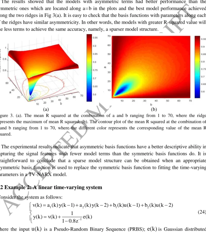
The results showed that the models with asymmetric terms had better performance than the symmetric ones which are located along a= b in the plots and the best model performance achieved along the two ridges in Fig 3(a). It is easy to check that the basis functions with parameters along each of the ridges have similar asymmetricity. In other words, the models with greater R-squared value will use less terms to achieve the same accuracy, namely, a sparser model structure.
(a) (b)
Figure 3. (a). The mean R squared at the combination of a and b ranging from 1 to 70, where the ridge represents the maximum of mean R squared; (b). The contour plot of the mean R squared at the combination of a and b ranging from 1 to 70, where the different color represents the corresponding value of the mean R squared.
The experimental results indicate that asymmetric basis functions have a better descriptive ability in capturing the signal features with fewer model terms than the symmetric basis functions do. It is straightforward to conclude that a sparse model structure can be obtained when an appropriate asymmetric basis function is used to replace the symmetric basis function to fitting the time-varying parameters in a TV-NARX model.
4.2 Example 2: A linear time-varying system
Consider the system as follows:
1 2 1 2 1 ( ) ( ) ( 1) ( ) ( 2) ( ) ( 1) ( ) ( 2) 1 ( ) ( ) ( ) 1 0.8 v k a k y k a k y k b k u k b k u k y k v k e k z (24)
where the input
u k
( )
is a Pseudo-Random Binary Sequence (PRBS);e k
( )
is Gaussian distributed noise with zero mean and variance 0.001, namely, with a 20dB SNR. The time-varying parameters are defined as:A
CCE
P
T
E
D
M
A
N
U
S
CRIP
T
1 2 1 0.32 cos(1.5 cos(4 )),1 4, ( ) 0.32 cos(3 cos(4 2)), 4 1 3 4, 0.32 cos(1.5 cos(4 )), 3 4 , ( ) 0.4 cos(4 ),1 , 0.65,1 4, 0.5, 4 1 2, ( ) 0.65, 2 1 3 4, 0.5, 3 4 1 , k N k N a k k N N k N k N N k N a k k N k N k N N k N b k N k N N k N 2( ) 0.6,1 , b k k N (25)respectively, where N2048 is the number of samples.
In order to identify a sparse model structure, an over-complete dictionary which consists of time-shifted alpha basis function is constructed. Assuming the support length of the basic alpha basis
function
( , 0,
k
a b
, )
, then the dictionary is defined as
1 1( , ,
, )
s m sD
k m
a b
,1,
,
k
N
is s,where, for simplicity, all the basis functions are set to have the same shape parameters a 3, b7, and scale . The scale was optimised in the identification by comparing the model performance under different scale parameters. This dictionary composes of an over-complete frame because there are a total number of Ns 1 N vectors in the dictionary.Dictionaries with more basis functions with different scales and shape parameters can be constructed. However, in this and following examples we restricted the dictionary to the simplest setting to illustrate the powerful descriptive ability of the new asymmetric basis function. The dictionary of process terms is constructed as
41
p d
D
y k d
. Therefore, the dictionary for the associated time invariant problem will be
,
, , ,
d m
D
k m
a b y k d , 1 d 4, s 1 m s1.Collecting the data and system (24) is identified using both OFR and LROFR algorithms. Results are shown in Fig 4 (c) and (d). The model performance is evaluated using the mean absolute error of the reconstructed time varying parameters, which is defined as
1 1 N ˆ k MAE c k c k c k N
(26)where
c k
andc k
ˆ
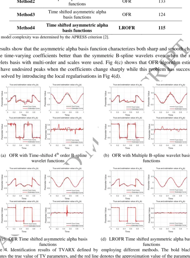
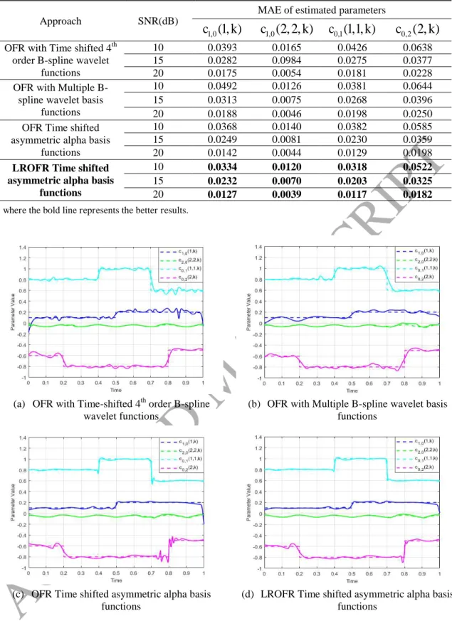
represent the original and identified model parameters, respectively.In order to illustrate the efficiency of the new proposed model. The results are compared with those of state-of-the-art methods [1, 4]. System (24) was also identified using multiple wavelet TVNAX model where the coefficients were approximated using symmetric B-spline wavelet basis function. The model dictionaries were organized in two different ways. In the first case, the wavelet basis functions constructed by time-shifting a basis 4th order B-spline wavelet as we did in the new proposed method. The results for this kind of model is shown in Fig 4 (a). Secondly, a multiple discrete B-spline wavelet basis was constructed including 3rd, 4th, and 5th B-spline wavelets with different scales. For more details, please refer to [4]. The results of this kind of model are shown in Fig 4(b). The four methods are summarized in Tab 1 and a comprehensive comparison of these four methods under different SNR levels are given in Tab 2.
Table 1. Summary of four TVNARX identification methods
Methods Basis functions Algorithm Model
A
CCE
P
T
E
D
M
A
N
U
S
CRIP
T
Method1 Time shifted 4th order B-spline
wavelet functions OFR 172 Method2 Multiple B-spline wavelet basis
functions OFR 133 Method3 Time shifted asymmetric alpha
basis functions OFR 124 Method4 Time shifted asymmetric alpha
basis functions LROFR 115
* The model complexity was determined by the APRESS criterion [2].
Results show that the asymmetric alpha basis function characterizes both sharp and smooth changes in the time-varying coefficients better than the symmetric B-spline wavelets even when the multi-wavelets basis with multi-order and scales were used. Fig 4(c) shows that OFR algorithm estimates may have undesired peaks when the coefficients change sharply while this problem has successfully been solved by introducing the local regularisations in Fig 4(d).
(a) OFR with Time-shifted 4th order B-spline wavelet functions
(b) OFR with Multiple B-spline wavelet basis functions
(c) OFR Time shifted asymmetric alpha basis functions
(d) LROFR Time shifted asymmetric alpha basis functions
Figure 4. Identification results of TVARX defined by employing different methods. The bold black line indicates the true value of TV parameters, and the red line denotes the approximation value of the parameters.
In order to validate the robustness and effectiveness of the new method, the four system identification approaches are compared under three different noise level, that is, SNR equals 20dB, 15dB, and 10dB. The simulations were run 100 times for each case with random noise. The mean MAE value over the 100 simulations is shown in Tab 2. The hyper-parameters, such as the model complexity and the wavelet scales, in each method, were optimised to produce the best performance.
A
CCE
P
T
E
D
M
A
N
U
S
CRIP
T
It can be observed that the proposed method with asymmetric alpha basis functions and LROFR algorithm is superior to the other methods using fewer terms and single wavelet scale. It is reasonable to believe that the new method may characterise the time-varying process better when multi-scale alpha basis function is used.
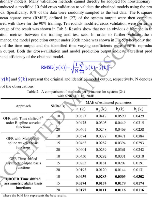
Model validation is essential and has been widely used for evaluating the efficiency of models or system identification algorithms. However, there are limited results on the model validation of nonstationary models. Many validation methods cannot directly be adopted for nonstationary cases. We conducted a modified 10-fold cross validation to validate the obtained models using the proposed methods. Specifically, 10% of the data were randomly sampled as the test data. The R squared and root mean square error (RMSE) defined in (27) of the system output were then computed and compared with those for the 90% training. Ten rounds modified cross validation were performed and the average of the result was shown in Tab 3. Results show that not an obvious difference in the two evaluation metrics between the training and test sets. In order to further validate the model performance, the model prediction output under 20dB noise was shown in Fig 5, where only the initial values of the time output and the identified time-varying coefficients were used to reproduce the system output. Both the cross-validation and model prediction output indicate excellent prediction power and efficiency of the obtained model.
2 11
Nˆ
kRMSE y k
y k
y k
N
(27)where
y k
andy k
ˆ
represent the original and identified model output, respectively. N denotes the length of the observations.Table 2. A comparison of methods performance for system (24) with SNR=10, 15, 20dB
Approach SNR(dB)
MAE of estimated parameters 1( )
a k a2( )k b k1( ) b k2( ) OFR with Time shifted 4th
order B-spline wavelet functions
10 0.0627 0.0412 0.0590 0.0429 15 0.0475 0.0305 0.0449 0.0315 20 0.0401 0.0248 0.0469 0.0258 OFR with Multiple
B-spline wavelet basis functions
10 0.0574 0.0377 0.0471 0.0384 15 0.0462 0.0287 0.0394 0.0293 20 0.0404 0.0239 0.0361 0.0242 OFR Time shifted
asymmetric alpha basis functions
10 0.0450 0.0292 0.0331 0.0310 15 0.0283 0.0181 0.0207 0.0191 20 0.0192 0.0120 0.0144 0.0131 LROFR Time shifted
asymmetric alpha basis functions
10 0.0439 0.0283 0.0303 0.0302
15 0.0274 0.0174 0.0179 0.0174
20 0.0177 0.0111 0.0116 0.0116
where the bold font represents the best results.
Table 3. Average model prediction error by cross validation for Example 2
SNR(dB) Train dataset Test dataset R squared RMSE R squared RMSE
A
CCE
P
T
E
D
M
A
N
U
S
CRIP
T
10 0.9570 0.1118 0.9346 0.1324 15 0.9843 0.0659 0.9731 0.0832 20 0.9946 0.0386 0.9794 0.0716Figure 5. The origin output and model prediction output under SNR = 20 dB in linear Example 2.
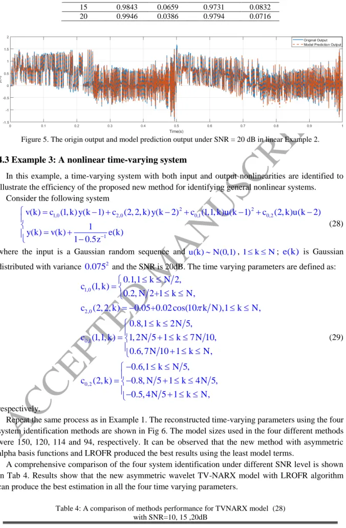
4.3 Example 3: A nonlinear time-varying system
In this example, a time-varying system with both input and output nonlinearities are identified to illustrate the efficiency of the proposed new method for identifying general nonlinear systems.
Consider the following system
2 2 1,0 2,0 0,1 0,2 1 ( ) (1, ) ( 1) (2, 2, ) ( 2) (1,1, ) ( 1) (2, ) ( 2) 1 ( ) ( ) ( ) 1 0.5 v k c k y k c k y k c k u k c k u k y k v k e k z (28)
where the input is a Gaussian random sequence and u k( )N(0,1), 1 k N; e k( ) is Gaussian distributed with variance 0.0752 and the SNR is 20dB. The time varying parameters are defined as:
1,0 2,0 0,1 0,2
0.1,1
2,
(1, )
0.2,
2+1
,
(2, 2, )
0.05+0.02 cos(10
),1
,
0.8,1
2
5,
(1,1, )
1, 2
5 1
7
10,
0.6, 7
10 1
,
0.6,1
5,
(2, )
0.8,
5 1
4
5,
0.5, 4
5 1
,
k
N
c
k
N
k
N
c
k
k N
k
N
k
N
c
k
N
k
N
N
k
N
k
N
c
k
N
k
N
N
k
N
(29) respectively.Repeat the same process as in Example 1. The reconstructed time-varying parameters using the four system identification methods are shown in Fig 6. The model sizes used in the four different methods were 150, 120, 114 and 94, respectively. It can be observed that the new method with asymmetric alpha basis functions and LROFR produced the best results using the least model terms.
A comprehensive comparison of the four system identification under different SNR level is shown in Tab 4. Results show that the new asymmetric wavelet TV-NARX model with LROFR algorithm can produce the best estimation in all the four time varying parameters.
A
CCE
P
T
E
D
M
A
N
U
S
CRIP
T
Approach SNR(dB)MAE of estimated parameters 1,0
(1, )
c
k
c
1,0(2, 2, )
k
c
0,1(1,1, )
k
c
0,2(2, )
k
OFR with Time shifted 4thorder B-spline wavelet functions
10 0.0393 0.0165 0.0426 0.0638 15 0.0282 0.0984 0.0275 0.0377 20 0.0175 0.0054 0.0181 0.0228 OFR with Multiple
B-spline wavelet basis functions
10 0.0492 0.0126 0.0381 0.0644 15 0.0313 0.0075 0.0268 0.0396 20 0.0188 0.0046 0.0198 0.0250 OFR Time shifted
asymmetric alpha basis functions
10 0.0368 0.0140 0.0382 0.0585 15 0.0249 0.0081 0.0230 0.0359 20 0.0142 0.0044 0.0129 0.0198 LROFR Time shifted
asymmetric alpha basis functions
10 0.0334 0.0120 0.0318 0.0522
15 0.0232 0.0070 0.0203 0.0325
20 0.0127 0.0039 0.0117 0.0182
where the bold line represents the better results.
(a) OFR with Time-shifted 4th order B-spline wavelet functions
(b) OFR with Multiple B-spline wavelet basis functions
(c) OFR Time shifted asymmetric alpha basis functions
(d) LROFR Time shifted asymmetric alpha basis functions
Figure 6. Identification results of TVNARX defined by (28) using four approaches. The dotted line with different color indicates the true value of TV parameters and the real line with the corresponding color denotes the approximation value of the parameters.
The same model validation processes as Example 2 have been performed and the results were shown in Tab 5 and Fig 7. It can clearly be observed that the proposed model has excellent performance in both identifying the model structure and capturing the changes in parameters.
A
CCE
P
T
E
D
M
A
N
U
S
CRIP
T
Table 5. Average model prediction error by cross validationfor Example 3
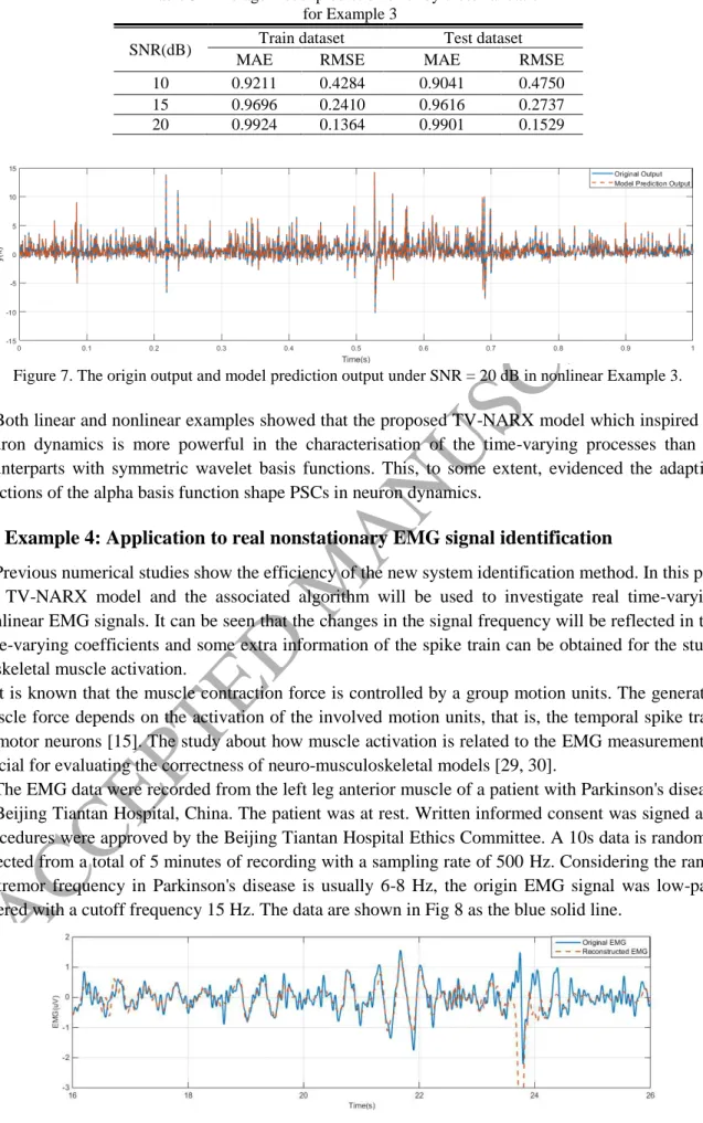
SNR(dB) Train dataset Test dataset MAE RMSE MAE RMSE 10 0.9211 0.4284 0.9041 0.4750 15 0.9696 0.2410 0.9616 0.2737 20 0.9924 0.1364 0.9901 0.1529
Figure 7. The origin output and model prediction output under SNR = 20 dB in nonlinear Example 3.
Both linear and nonlinear examples showed that the proposed TV-NARX model which inspired by neuron dynamics is more powerful in the characterisation of the time-varying processes than its counterparts with symmetric wavelet basis functions. This, to some extent, evidenced the adaptive functions of the alpha basis function shape PSCs in neuron dynamics.
4.4 Example 4: Application to real nonstationary EMG signal identification
Previous numerical studies show the efficiency of the new system identification method. In this part, the TV-NARX model and the associated algorithm will be used to investigate real time-varying nonlinear EMG signals. It can be seen that the changes in the signal frequency will be reflected in the time-varying coefficients and some extra information of the spike train can be obtained for the study of skeletal muscle activation.
It is known that the muscle contraction force is controlled by a group motion units. The generated muscle force depends on the activation of the involved motion units, that is, the temporal spike train of motor neurons [15]. The study about how muscle activation is related to the EMG measurement is crucial for evaluating the correctness of neuro-musculoskeletal models [29, 30].
The EMG data were recorded from the left leg anterior muscle of a patient with Parkinson's disease at Beijing Tiantan Hospital, China. The patient was at rest. Written informed consent was signed and procedures were approved by the Beijing Tiantan Hospital Ethics Committee. A 10s data is randomly selected from a total of 5 minutes of recording with a sampling rate of 500 Hz. Considering the range of tremor frequency in Parkinson's disease is usually 6-8 Hz, the origin EMG signal was low-pass filtered with a cutoff frequency 15 Hz. The data are shown in Fig 8 as the blue solid line.
A
CCE
P
T
E
D
M
A
N
U
S
CRIP
T
Figure 8. A comparison of the real EMG data and reconstructed data established by TV-NARX model (31), where the bold black line denotes the original EMG signal while the red line is the fitting line.The initial guess of the TV-NARX model structure was chosen as
4 4 4 1 0 2,0 0,0 1 1 1( )
( , ) (
)
( , , ) (
) (
)
( )
i i jy k
c
i k y k i
c
i j k y k i y k
j
c
k
e k
(30)including 15 candidates process terms. The asymmetric alpha basis functions were used to fit the time-varying parameters. The LROFR algorithm is adopted to select the significant terms. Results showed that only linear terms are significant in the description of the EMG dynamics and the obtained model is given as (31). 4 1 0 1
( )
( , ) ( - )
( )
iy k
c
i k y k i
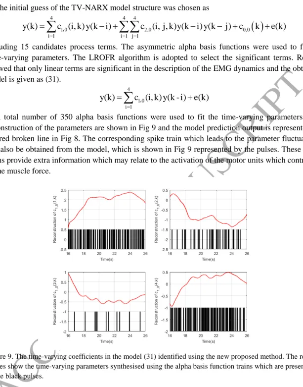
e k
(31)A total number of 350 alpha basis functions were used to fit the time-varying parameters. The reconstruction of the parameters are shown in Fig 9 and the model prediction output is represented by the red broken line in Fig 8. The corresponding spike train which leads to the parameter fluctuations can also be obtained from the model, which is shown in Fig 9 represented by the pulses. These spike trains provide extra information which may relate to the activation of the motor units which contribute to the muscle force.
Figure 9. The time-varying coefficients in the model (31) identified using the new proposed method. The red curves show the time-varying parameters synthesised using the alpha basis function trains which are presented as the black pulses.
4.5 Example 5:
Application in the detection of freezing of gait in Parkinson’s disease
In this part, the proposed TV-NARX model with asymmetric alpha basis function expansion was
used to modelling the nonstationary gait data of Parkinson’s disease where the accelerations in
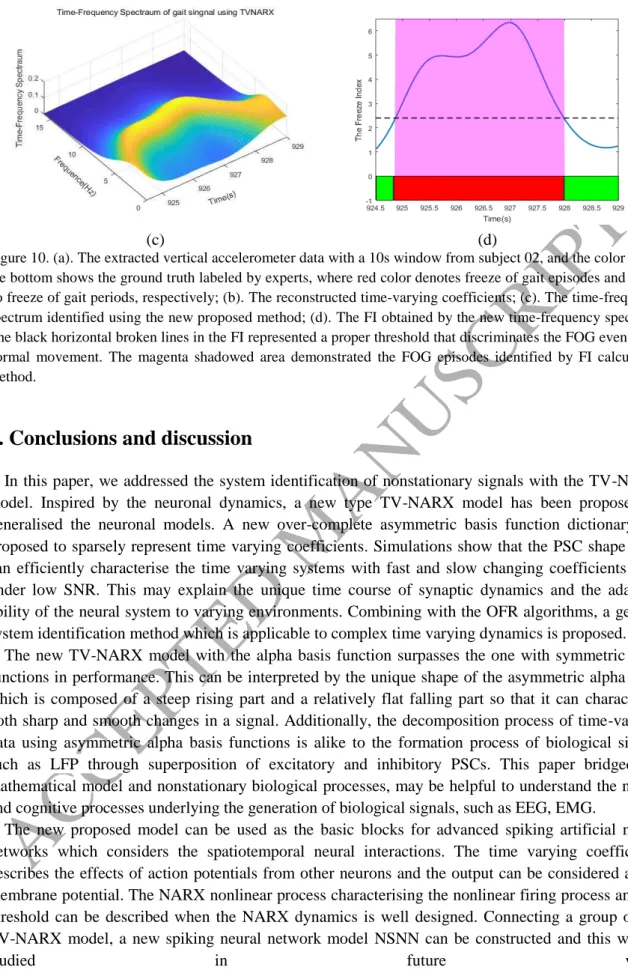
Daphnet Freezing of Gait Dataset were used [31]. A typical 4.5s vertical accelerometion at the ankle including both normal locomotion and freezing of gait were low pass filtered and the preprocessed data are shown in Fig 10(a).
By selecting the significant terms using the LROLR algorithm, a second order linear time varing model of form (32) was obtained
A
CCE
P
T
E
D
M
A
N
U
S
CRIP
T
2 1 0 1 ( ) ( , ) ( - ) ( ) i y k c i k y k i e k
(32)A total number of 89 alpha basis functions were selected to fit the two time-varying parameters and the reconstructed parameters was shown in Fig 10(b).
Unlike purely phenomenological models, TV-NARX models can provide an explicit model structure and can be used for further model based analysis. In this example, the obtained TV-NARX model was then used to estimate the time varying time-frequency spectrum of the gait data according to formula (33): 2 2 2 2 1,0 1
1
( , )
1
( , )
s TDS e j if f iP
k f
c
i k e
(33)where PTDS( , )k f is the time-frequency spectral estimation value at continuous independent variables time k and frequency f, cˆ1,0( , )i k is the estimation of model parameters c1,0( , )i k , 2
e
is the variance of model residual, fs= 64Hz is the sampling frequency and j -1 denotes the imaginary part of a complex number.
Results have shown that the model based method is capable of providing a time-frequency spectrum with high resolution in both time and frequency domain [32]. The obtained time-frequency spectrum which characterises the variation of frequency components over time is shown in Fig 10(c).
A biomarker, namely, Freeze Index (FI) [33] for the detection of FOG can then be defined based on the time-frequency spectrum as the ratio of energy in freezing band (3-8Hz) and normal locomotion band (0.5-3Hz). The calculated FI using formula (34) is shown in Fig 10 (d).
8 3 3 0.5
( , )
( )
( , )
TDS TDSP
k f df
FI k
P
k f df
(34)The results in Fig 10(b,c,d) showed that the FI can accurately detect the occurrence of the FOG. The trend of parameters and time-frequency spectrum is consistent with the occurrence of FOG episodes in Fig 10(b,c). Based on the new proposed method a convenient framework can be constructed for discriminating FOG events easily and accurately.