Managerial Economics 2013, No. 14, pp. 17–38
http://dx.doi.org/10.7494/manage.2013.14.17
Henryk Gurgul*,1Artur Machno*, Robert Syrek**2
The optimal portfolio
in respect to Expected Shortfall:
a comparative study
1. Introduction
Dependence structures in capital markets have recently attracted increasing attention among economists, empirical researchers, and practitioners. In order to control a portfolio for risks, portfolio managers and regulators have to take into account a degree of dependence between international equity markets when studying returns across international financial markets. Therefore, the topic of asymmetric dependence structures, such as high dependence in a bear period of the stock market is very important for both the risk control and the policy man-agement. In addition, the benefits derived from an international diversification of asset allocation are often affected by asymmetric dependence structures.
It is well known and widely discussed in the literature that linkages among international capital markets are mostly asymmetric. From this asymmetry re-searchers draw a conclusion that in a bear phase, returns tend to be more inter-related than they are in a bull phase of capital markets. From this observation serious theoretical consequences for an international portfolio follow. The most important implication is a possible loss of diversification benefits in a bear time due to the rise in the dependence among capital markets. In other words, inter-national portfolios become much more risky in bad times of stock markets that assumed in good times. The observed asymmetric dependence is an essential source of rise in the costs of a diversification with foreign equities.
* AGH University of Science and Technology in Cracow, Department of Applications of Mathematics in Economics, e-mail: [email protected]; [email protected]
Financial support for this paper from the National Science Centre of Poland (Research Grant DEC-2012/05/B/HS4/00810) is gratefully acknowledged by Henryk Gurgul.
In this article we investigate how model selection affects the calculated risk of financial position. The two standard models are mean-variance Markowitz model and multivariate GARCH model. Both models assume symmetric and thin-tailed distributions of returns, in particular they assume the normal distribution. Recently developed models based on copula functions are both flexible and con-venient to model anomalies in distributions, such as an asymmetry or fat-tails. In this article we focus on regime switching copula models. We consider two risk measures: Value at Risk and Expected Shortfall. The expected risk derived on the basis of the regime switching copula model is compared to the expect risks ob-tained by using the Markowitz model and the multidimensional GARCH model.
A model misspecification may cause a number of problems. Incorrect evalua-tion of the expected value of a financial posievalua-tion is one of the most serious draw-backs of the financial models. However, a risk underestimation may cause even worse consequences. Most of risk measures are strongly, or entirely, dependent on distributions of tails. Especially, the dependence of extreme assets’ values substantially affects the distribution of the portfolio value. Therefore, an omis-sion of an asymmetry or a high kurtosis of assets’ distributions may be a reason for a miscalculation of risks.
The remainder of the contribution is organized in the following way: in sec-tion 2 we conduct the literature overview concerning the dependence concepts, including regime switching models and copulas and discuss the recent contribu-tions to the subject; in section 3 the dependence measures and copulas are over-viewed; in the following section the copula regime switching model is described; in the fifth section risk measures based on copula models are discussed; in the sixth section we present the data, report and discuss the results; section 7 con-cludes the paper.
2. Literature overview
Relations among international stock markets have been investigated in many papers, especially in the period of the financial crises. The topic under study is important for market participants, because, due to the globalization process, the global markets are becoming more and more dependent. This observation follows from the liberalization and deregulations in both money and capital markets. In addition, the globalization process diminishes opportunities for international diversification.
Numerous recent studies deal with an asymmetry in dependence structures in international stock markets. They reveal two interesting asymmetries. The de-pendence tends to be high in both highly volatile markets and bear markets.
The optimal portfolio in respect to Expected Shortfall: a comparative study
While in some studies, the evidence of the first type of asymmetry is shown, several other studies found the second asymmetry. In one of the earliest contribu-tion, Hamao, Masulis, and Ng [18] investigated the relations among equity mar-kets across Japan, the U.K., and the U.S. using the daily data of stock indices. The authors estimated the GARCH-M model. Using this model the authors established volatility spillover effects from the U.S. and U.K. stock markets to the Japanese market. King and Wadhwani [23] developed a contagion mechanism model. They detected contagion effects. The contributors stressed that an increase in volatility by using a high frequency data from the stock markets in Japan, the U.K., and the U.S strengthened these effects. These findings were supported to some extent by Lin et al. [26] who analysed two international transmission mechanism models based on the daily returns of stock indices in Japan and the U.S. Erb et al. [14] found that monthly cross-equity correlations among the G7 countries were high-est when any of two countries were in a recession. In addition, the contributors claimed that they are much higher in bear markets. In the paper by Longin and Solnik [27], the monthly data of stock indices for several industrial countries were analyzed. The contributors, using a multivariate GARCH model, found that the correlations between major stock markets raised in periods of a high volatil-ity. On a basis of the multivariate SWARCH model, Ramchand and Susmel [36] found that monthly returns of stock markets in the U.K., Germany, and Canada tended to be essentially more correlated with the U.S. equity market during pe-riods of a high U.S. market volatility. The similar results could be found in King, Sentana, and Wadhwani [22], Ball and Torous [5], Bekaert and Wu [6], Ang and Bekaert [2], and Das and Uppal [10].
Following Davison and Smith [11] and Ledford and Tawn [25], Longin and Solnik [28] derived a method to measure the extreme high correlation by the conditional tail correlation based on extreme value theory. The contributors es-tablished that the conditional correlation between the U.S. and other G5 coun-tries strongly increases in bear markets. In contrary, the conditional correlation does not essentially increase in bull markets.
In more recent studies by Campbell et al. [7], Ang and Bekaert[2], Das and Uppal [10], Patton [34], and Poon et al. [35], the existence of two regimes in international equity markets was suggested: a high dependence regime with low and volatile returns and a low dependence regime with high and stable returns.
Based on this hypothesis, Ang and Bekaert [2] estimated a Markov switch-ing multivariate normal (MSMVN) model usswitch-ing the U.S., the U.K., and German monthly stock indices. The contributors detected some evidence that a bear regime is characterized by low expected returns, high volatility, and high cor-relation, whereas a normal regime is characterized by high expected returns, low volatility, and low correlation. Their model was able to replicate Longin and
Solnik’s [28] results. Referring to Ang and Chen [2], they demonstrated that an asymmetric bivariate GARCH model, widely used in the literature to analyze the international stock markets, cannot replicate them.
In recent times, copulas have become a major tool in the finance for model-ling and analyzing dependence structures between financial variables. In contrast to the linear correlation, the copula reflects the complete dependence structure inherent in a random vector (see [13]). In finance, copulas have attracted much attention in the calculation of the Value-at-Risk (VaR) of market portfolios (see e.g. Junker and May, 2005; Kole et al., 2007 and Malevergne and Sornette, 2003) and the modelling of the credit default risk.
Ball and Torous [5] and Guidolin and Timmermann [17] investigated the economic significance of their empirical findings from a risk management point of view. Rodriguez [37] used copula model with Markov switching parameters. Okimoto [32] stressed that ignoring the asymmetry in bear markets could be costly when risk measures are evaluated. In his contribution, using a copula based regime switching Markov model, he concentrated on the value at risk (VaR) and expected shortfall (ES).
According to his calculation, ignoring such an asymmetry in bear markets significantly affects risk measures, i.e. the 99% VaR is undervalued by about 10%, while the expected shortfall is undervalued by about 5% to 10% consistently over the whole significance level between 90% to 99%. This is essential for the risk management.
The empirical literature on the optimal choice of the parametric copula fam-ily for the VaR-estimation can be clustered into three groups.
The first group of contributors claims that the elliptical copulas are opti-mal. The representative of this stream of papers is e.g. paper by Malevergne and Sornette [29]. This is one of the first empirical studies on the optimality of cop-ula models for the modelling of dependence structures of linear assets. The au-thors, based on the dataset consisting of six FX futures, six commodity prices and 22 stocks listed on the NYSE, demonstrated that the dependence structures of the majority of bivariate portfolios built from these assets can be correctly reflect-ed by a Gaussian copula. However, in the opinion of the contributors, their result can be biased. The reason is that Student’s t copula can easily be mistaken for a Gaussian copula. In addition, Malevergne and Sornette [29] did not include the estimation of a risk measure or Goodness of Fit –tests (abbreviation GoF-tests). Kole et al. [24] found, on the basis of just one trivariate portfolio (one stock-, one bond- and one REITS-index), that the Student’s t copula is the best for modelling the dependence structure of linear assets. DiClemente and Romano [12] using the 20-dimensional portfolio of Italian stocks, demonstrated that a model incor-porating margins following an extreme value distribution and an elliptical copula
The optimal portfolio in respect to Expected Shortfall: a comparative study
can yield much better VaR-estimates than the classical correlation-based model. However, they used neither Archimedean copulas nor copula-GoF- tests. In con-tribution by Fantazzini [15], it is shown that three bivariate portfolios built from stock indices can be well modelled by a constant or dynamic Gaussian copula in order to estimate VaR properly.
The second stream of studies justifies an optimality of Archimedean copu-las. Junker and May [21] argued that a transformed Frank copula with GARCH margins can improve VaR- and ES-estimates in comparison to elliptical copula models. However, their conclusions are based solely on the single bivariate port-folio of German stocks. In addition, they only apply GoF-tests for general distri-butions. They were not adjusted to the characteristics of copulas. Similar results were presented by Palaro and Hotta [33] for the bivariate portfolio based on the S&P 500- and the NASDAQ- index. The authors showed that a symmetrised Joe-Clayton copula joint with GARCH margins performs significantly better than elliptical copula models.
Recent studies, belonging mostly to a third cluster of research, demonstrate that the optimal parametric copula as well as the strength and structure of the dependence between asset returns are not constant over the time. In order to allow the parametric form of the copula to change over time more recent studies like the ones addressed above Rodriguez [37], Okimoto [32], Chollette, Heinen, and Valdesogo [8] and Markwat, Kole, and van Dijk, [31], Weiss [38] apply the convex combinations of copulas. The contributors drew a conclusion that more flexible mixture copula models yield better VaR and ES estimates than uncondi-tional copula models.
The contributors stressed that copula models perform better than correla-tion-based models with respect to the estimation of VaR. This was the case when the optimal parametric copula family was known ex ante.
The main aim of this contribution is a comparison of the expected shortfall for returns derived on the basis of the Markowitz model, the multidimensional GARCH model and the copula regime switching model.
3. Dependence measures based on copulas
The correct evaluation of the dependence between assets’ interest rates is essential for an accurate assessment of an investment risk. In the case of risk management, the dependence between negative values, in particular between extreme negative values plays a key role. Especially, if such a dependence is substantial, then an investor can lower the risk by diversification of a portfolio to less than expected. In this section we present some functions measuring the dependence between
random variables and discuss their intuitive meaning. Moreover, we describe the presented dependence measures’ relationship with copulas.
3.1. Exceedance correlation coefficient
The most traditional dependence measure is Pearson correlation. However, it measures only linear dependence and works only in the range of the spheri-cal and elliptispheri-cal distributions. The exceedance correlation is the generalized Pearson coefficient which measures asymmetric dependence. It is defined as the correlation between two variables, conditional on both variables being below or above some fixed levels. Exceedance correlation coefficients between random variables X and Y are defined as:
T T T T d T d T t T t T 1 2 1 2 1 2 1 2 | | , : , , , , : , , , L U ecorr X Y corr X Y X Y ecorr X Y corr X Y X Y (1) (2) where ecorrT T1 2Lis lower exceedence correlation, T T1 2 U
ecorr is upper exceedence cor-relation and LJ1, LJ2 are fixed thresholds.
Properly calculated exceedance correlation would be an efficient tool in risk management, where negative extreme values of an investment return are crucial. However, this coefficient has some drawbacks. For instance, it is computed only from observations which are below (above) the fixed limit. Therefore, as the limit is further out into the tail as exceedance correlation is computed less precisely. Another inconvenience with the exceedance correlation is that it is dependent on margins, thus it cannot be calculated only from the copula connecting variables.
3.2. Tail dependence
Another tail dependence measure is quantile dependence. For random variables X and Y with distribution functions F and G, respectively, the lower tail dependence at threshold Įis defined as ª¬ 1 D_ 1 D º¼
P Y G X F . Analogously,
the upper tail dependence at threshold Į is defined as m ª¬ ! 1 D_ ! 1 D º¼
P Y G X F .
The dependence measure which is particularly interesting is the tail dependence obtained as the limit of a quantile dependence. We define lower tail dependence NJL of X and Y as: Do ª º O ¬ 1 D 1 D ¼ 0 c L limP Y G _X F , (3)
and upper tail dependence Ưu of X and Y as: Do ª º O ¬ ! 1 D ! 1 D ¼ 1 c U limP Y G _X F . (4)
The optimal portfolio in respect to Expected Shortfall: a comparative study
Variables X and Y are called asymptotically dependent if NJL (0,1] and as-ymptotically independent if NJL = 0For variables connected by the copula C, lower tail dependence NJL and upper tail dependence NJU can be computed as follows:
o O 0 , lim , L u C u u u (5) o O 1 1 , lim , U u C u u u (6)
where C is the survival copula defined by:
, 1 ,1 1 ,
C u v C u v u v u for u,u (0,1] (7) Unlike exceedance correlations, tail dependence is independent ofmargins. In the most cases, for a given copula, one can simply calculate tail dependences using formulas (5) and (6). In Table 1, we present results for the copulas used in the paper.
Table 1
Tail dependencies for Gaussian, BB1, BB4, BB7 copulas
NJL NJU Gauss Ǐ C 0 0 , LJį CBB1 1 2GT 1 2 2 G 4 , BB LJį C 1 1 2 2G T § · ¨ ¸ © ¹ 1 2G 7 , BB LJį C 1 2G 1 2 2 T 3.3. Kendall’s IJ
Another class of dependence measures is based on ranks of variables. The two most popular rank correlations coefficients are Kendall’s IJ and Spearman’s Ǐ Both rely on the notion of the concordance. Let (x1, y1) and (x2, y2) be two observations of the random vector (X, Y). We say that the pair is concordant whenever (y1 – y2)(x1 – x2) > 0 , and discordant whenever (y1 – y2)(x1 – x2) < 0. Intuitively, a pair of random variables are concordant if large values of one vari-able occur more likely with large values of the other varivari-able.
For random variables X and Y, Kendall’s IJ is defined as:
ª º ª º
where (x1, y1) and (x2, y2) are independent observations of (X, Y). In terms of copulas, Kendall’s IJhas concise form. For the pair of random variables X and Y and its copula C, we have:
W
³
2 0 1 4 1 [ , ] , , . C C u v dC u v (8)Since copula is invariant with respect to any monotonic transformation, Kendall’s IJ has also this property. From the formula (8) we see that Kendall’s IJ does not depend on marginal distributions.
4. Compared models
In this section we present the regime switching copula model with GARCH margins and the estimation procedure. Other models used in this article are: the Markowitz model and multivariate Generalized Autoregressive Conditional Heteroscedasticity (mGARCH) model.
The Markowitz model is a standard model introduced by Markowitz. This model is based on a normal distribution assumption and does not include any dynamic changes. There are numerous papers stressing the inadequacy of this model. We believe that there are still individuals using this method. Thus, we decided to compare this method to other in the context of our study. Markowitz model’s parameters can be equivalently estimated using the likelihood function maximization or the least square method.
Switching models were introduced by Hamilton [19] and widely analyzed by Hamilton [20]. Let yt =(y1t, y2t) be a pair of interest rates of analyzed indices, and let Yt =(yt, yt–1, yt–2,...) be the series of observations available at the time t.
We denote the two-state Markov state process by st, which has two possi-ble values, say 1 and 2, we call these states regimes. We choose the first regime copula from copulas with non-zero tail dependencies, namely BB1, BB4 and BB7 copulas. The second copula is the Gaussian copula, which corresponds to sym-metry and tail independence of the investigated variables.
The conditional joint density function f for yt is defined as:
| 1, 1( 1;G1), 2( 2;G 2) 1( 1;G 1) 2( 2 ;G2), jt t t t t t t
f y Y s j c F y F y f y f y (9)
where Fi and fi, for i = 1,2 , are the marginal distribution functions and density functions of corresponding variables, and įi is a parameter vector for the mar-ginal distribution. The probability that the state i precedes the state j is denoted by Sij = P[st = j|st–1 = i].
The optimal portfolio in respect to Expected Shortfall: a comparative study
All four probabilities form transition matrix:
ª º « » ¬ ¼ 11 12 11 21 22 1 S S S S S S P ª« º» ¬ ¼ 11 22 22 1 S S . (10)
The estimation of the regime switching copula model is based on the maximum likelihood estimation. Unfortunately, the computing power need-ed to maximize likelihood function is enormous. To simplify the calculation, the decomposition of likelihood function to margins likelihood functions and the dependence likelihood function is performed. Formally, for a given sample
Y=(Y1, Y2,..., YT) , the log-likelihood function is defined by:
G T¦
1 G T 1 ln ; , ( | ; , ), T t t t L Y f y Yand it is decomposed to Lm and Lc such that:
; ,G T m;G c ; ,G T, L Y L Y L Y where: ª º G
¦
¬ 1 1 1 1 G 1 2 2 2 1 G2 ¼ 1 ln ln | ; | ; ; , T m t t t t t L Y f y Y f y Y (11) G T¦
1 1 11 G1 2 2 21 G T¼2 º 1 ln | ; , [ |( ; , ; ; . T c t t t t t L Y c F y Y F y Y (12)The parameters of the model are estimated as follows. In the first step we estimate the parameters į1 and į2 of the marginal distribution. This step is per-formed by the maximization of the likelihood function defined by (11). In the second step we maximize the likelihood function defined by (12) to estimate parameters LJ1 and LJ2 of copulas c(1)and c(2), and transition matrix given by (10). Note that parameters į1,į2,LJare in fact collections of parameters.
A method of the estimation of marginal distributions depends on the model which is chosen to describe the specific marginal variable. To model the mean of a time series, we use the simple autoregressive model. As we mentioned before, usually for time series of returns hypotheses of normal distribution of residuals are rejected. In particular, investigated time series are fat-tailed, asymmetric and heteroscedastic. Therefore, for every analyzed time series rt, we use the following AR(1)-GARCH(1,1) model: M M0 1 1 H t t t r r (13) Z DH E2 1 1 t t t h h for Z!Dt, Et; (14)
where İt= ht et and et is a white noise. Although, with respect to an asymmetry and a fat tail, et is described by the skewed Student-t distribution. The skewed
Student-t is a two parameter distribution. For v ! 2 and NJ[–1,1], the skewed Student-t density function, denoted by St, is defined by:
Q Q O Q § § · · ° ¨ ¸ ¨ ¸ ° ¨ Q © O ¹ ¸ ° © ¹ ® ° § § · · ° ¨ ¨ ¸ ¸ t ¨ ¸ ° © Q © O ¹ ¹ ¯ 1 2 2 1 2 2 1 1 dla 2 1 1 1 dla 2 1 ( ) , ( ) ( ) , bx a a bc x b St x bx a a bc x b (15) where
Q § · *¨ ¸ Q § · © ¹ O ¨ ¸ O Q § · © ¹ S Q *¨ ¸ © ¹ 2 2 1 2 2 4 1 3 1 2 2 , , , a c b a c vThe second step is the estimation of copulas parameters and transition prob-abilities. To do so, we use Hamilton filter. For the transition matrix P given by (10), we define: [ K [ [ K : : 1 1 1 | | | , ˆ ˆ ˆ ( ) t t t t t T t t t (16) [ 1| [| ˆ Tˆ , t t P t t (17) where [ ˆt t| P s[ t j Y| t; ]T and ˆ[t1|t P s[ t1 j Y| t; ]T the Hadamard’s multipli-cation denoted by : means the multiplication coordinate by coordinate. The vector of copulas’ densities is denoted by džt,
1 1 1 1 2 2 2 1 2 1 1 1 2 2 2 2 ª G G T º « » K G G T « » ¬ ¼ ( ; , ; ; ) . ( ; , ; ; ) t t t t t c F y F y c F y F y (18)The log-likelihood function defined by (12) for the observed data can be written as:
1 1 ln 1 G T¦
[| :K ; , ˆ , T T c t t t t L Y (19)where the initial value[ˆt1|0 is the limit probability vector:
22 11 22 1 0 11 11 22 1 2 1 2 ª º « » « » [ « » « » ¬ ¼ | ˆ p p p p p p (20)
The optimal portfolio in respect to Expected Shortfall: a comparative study
Models based on mGARCH have been recently broadly used and modified. In this article, conditional mean dynamics is described by the VAR(1) model. For details of the recent study we refer to Croux and Joossens [9]. To model condi-tional correlation, we use the Dynamic Condicondi-tional Correlation (DCC) model with normal conditional distributions.
Under this model the conditional mean of the multidimensional time series
y at the time t is computed as follows:
1 1
yt Ayt
[ | ]
( t P HHt, (21)
where Njis constant, ƻt is the information set available at the time t and is a vec-tor auvec-toregressive matrix. The error term İt at the time t is defined by:
Ht Ht zt, ( / )1 2
(22)
where zt is a sequence of N- dimensional, in our case N = 2, i.i.d. random vector
with the following characteristics: E(zt) = 0 and t t T
N
E z z I , therefore zt~N(0, IN).
The dynamic covariance matrix Ht is decomposed to:
Ht = Dt Rt Dt, (23)
where Dtis a dynamic variance matrix and Rt is a dynamic correlation matrix. In
the two-dimensional case, Dt diag
h11,t, h22,t, where1
t t
h Z DH :H Et1 ht1. (24)
The correlation matrix Rt is decomposed as follows:
^
`
1^
`
12 2
diag( ) diag( ) .
t t t t
R Q Q Q (25)
The correlation driving process Qt is defined by:
*1 1
1 ,
t t t
Q D E Q DP EQ (26)
where Q denotes unconditional correlation matrix of the stantarized errors and
^
`
1^
`
1* diag( ) 2 1 1 diag( ) 2.
t t t t t t
P Q D Q D Q (27)
This particular specification of the DCC model has been proposed by Ailelli [1].
5. Portfolio optimization
The portfolio optimization problem is widely analyzed. There are two main goals to achieve in any portfolio optimization problem. The first aim is the maximi-zation of the expected value of the portfolio. The most natural way is to maximize
the expected nominal value, a generalization of this approach is the maximization of an expected utility. In this article, we do not consider utility functions, for more details about a maximizing an expected utility see Föllmer and Schied [16]. The second aim in the portfolio optimization is to minimize a risk. There are numer-ous approaches to a concept of risk. The most standard understanding of a risk is an uncertainty. For any portfolio, its risk may be understood as the variance of the future value of the portfolio. This concept was firstly introduced in [30] and the corresponding portfolio optimization problem was solved in this paper.
In this article, we deal with the concept of risk proposed in [4]. We analyze the risks of the financial positions in the one period case. It means that the value of the financial position under study in the end of the period turns into a random variable.
The function Ǐ: 0 o, where 0 is the family of all attainable financial posi-tions, is called risk measure if it satisfies the following properties for all financial positions X, Y:
1.Monotonicity:
If Xd Y, then Ǐ(X) tǏ(Y). (28)
2.Cash invariance:
If m, then Ǐ(X + m) = Ǐ(X )– m. (29)
The interpretation of monotonicity is clear: The increase of a financial posi-tion’s payoff profile do not increase its risk. The cash invariance is motivated by the interpretation of Ǐ(X) as a capital requirement. If the amount m is added to
the position and invested in a risk-free manner, the capital requirement is re-duced by the same amount.
It is usually assumed that the portfolio diversification should not increase the risk. Convex risk measures has this property, the risk measure Ǐ is called con vex risk measure if it satisfies the following convexity property for all financial positions X, Y:
X 1 YX 1 ( ),Y
U O O d OU O U , for all 0 dNJd. (30) Moreover the convex risk measure Ǐ is called coherent risk measure if it satisfies the following positive homogeneous property:
,
X X
U O d OU , for all 0 dNJ and X 0. (31) Value at Risk (VaR) is an approach to the problem of measuring the risk of a financial position X based on specifying a quantile of the distribution of X un-der the given probability measure. Value at Risk is the smallest amount of capital which, if added to X and invested in the risk-free asset, keeps the probability of a negative outcome below some fixed level.
The optimal portfolio in respect to Expected Shortfall: a comparative study
For X 0 and NJ (0,1) we define Value at Risk at level NJas:
VaRNJ (X) ؔ inf
^
m|P[X d Om 0]`
. (32) In the other words, VaRNJ (X) is (1 – NJ)-quantile of the variable (–X). Clearly,VaR is a positively homogeneous risk measure. Generally, Value at Risk is not a convex risk measure. However, it is convex if it measures a risk of financial posi-tions come from some particular classes. For instance, VaR is convex risk measure if X consists of only normally distributed financial positions.
This risk measure has a clear interpretation and is recommended by numer-ous financial institutions and presented in documents such as the Basel Accords. However, the absence of the convexity is a substantial objection. This disadvan-tage of VaR led researchers to convex risk measures which have similar inter-pretation as Value at Risk. It appears that, so called ([SHFWHG6KRUWIDOO(ES), is a convex risk measure.
For X 0 and NJ (0,1) we define ([SHFWHG6KRUWIDOODWOHYHONJ as:
ESNJ (X) ؔ E[VaRD|D dO] (33) This convex risk measure is also called Conditional Value at Risk (CVaR),
Average Value at Risk (AVaR), Tail Value at Risk (TVaR), Mean Excess Loss or Mean Shortfall. However, there are other risk measures defined in some papers under these names. In this article, the risk measure defined by (33) is called an Expected Shortfall. Clearly, ESNJ(X) tVaRĮ, for any NJ (0,1).
In general case it is difficult or impossible to find an analytical form of
ES. One can notice that there does not exist an analytical form of VaR for normally distributed financial positions. We estimate VaR using the Monte Carlo method. For every analyzed model, we simulate 1,000,000 observations. It is usually rec-ommended to simulate 100,000 observations. However, we are mostly interested in extreme observations, namely those which are below VaRNJ-level. In the formula (33), one can see that ESNJ is determined by a conditional distribution, in particu-lar by the financial position’s distribution in the lower NJ-tail.
6. The data and the estimation results
The database consists of prices of three stock market indices. Namely, the American DJIA, the German DAX and the Austrian ATX. In order to avoid intro-ducing an artificial dependence due to the difference in closing times of stock exchanges around the globe, we work with Wednesday to Wednesday returns. Comparing to daily returns, weekly return processes have lower autocorrelation
and avoid the missing data problem. This gives us a sample of 689 weekly returns from January 2000 to March 2013. We apply continuous (logarithmic) returns:
1 100 log t t t S r S
,
(34)where Stis the price index at the time t.
Firstly, we present some descriptive statistics in Table 2.
Table 2
Logarithmic rates of return time series summary statistics
ATX DAX DJIA
Mean 0.1036 0.0248 0.0335
Median 0.4157 0.3984 0.2140
Std. dev. 3.4646 3.4630 2.5782
Kurtosis 16.7931 5.1127 7.7125
Skewness –1.9245 –0.6643 –0.9464
In the period under study we observe an insignificant positive means in all the three indices. A relatively large absolute value of median suggest asym-metries in the examined time series. Negative skewnesses confirm this con-jecture. These asymmetries suggest that normal distribution should not be used to model these time series, and high kurtosis in all the three time series confirms that.
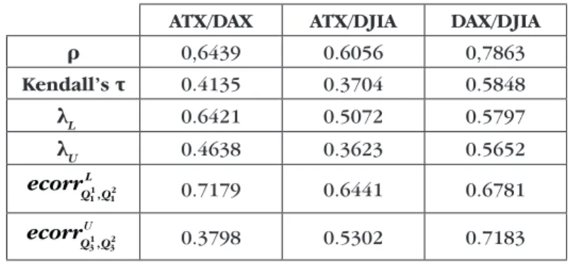
Table 3 presents empirical dependence measures for analyzed pairs of price indices.
Table 3
Empirical dependences between price indices’ time series
ATX/DAX ATX/DJIA DAX/DJIA
Ǐ 0,6439 0.6056 0,7863 Kendall’s IJ 0.4135 0.3704 0.5848 NJL 0.6421 0.5072 0.5797 NJU 0.4638 0.3623 0.5652 1 2 1, 1 L Q Q ecorr 0.7179 0.6441 0.6781 U 1 2 3, 3 Q Q ecorr 0.3798 0.5302 0.7183
The optimal portfolio in respect to Expected Shortfall: a comparative study
Here Ǐ is Pearson’s correlation, QD1 and 2
QD are Į-quartiles of a realized vola-tility series and a daily volume series, respectively. Tail dependencies NJL and NJU are
approximated by P Yª G1 0.1 |X F1 0.1 º
¬ ¼ and P Yª¬ !G1 0.9 |X!F1 0.9 º¼, respectively.
One can observe the strong and significant linear correlation between the indices under consideration. As expected, the strongest dependence is observed for the DAX/DJIA pair. Despite the many drawbacks of linear correlation, it is worth to mention that a portfolio construction is very sensitive to the degree of dependence.
Asymmetries in tails are observed for the ATX/DAX and ATX/DJIA pair. For the DAX/DJIA pair, the lower and the upper estimated tail dependence are at similar levels. The same result is observed for exceedence correlations.
A multidimensional GARCH(1,1) model with conditional mean described by the VAR(1) is supposed to eliminate the incorrect assessments of the foregoing model. Table 4 presents A matrices and constants Njfrom equation (21) for the three pairs of analysed time series:
Table 4
Vector autoregressive parameters
ATX DAX ATX DJIA DAX DJIA
ATX –0.0738 0.0855 ATX –0.1274 0.2409 DAX –0.0937 0.0880
DAX –0.0640 –0.0009 DJIA –0.0006 –0.0754 DJIA –0.0265 –0.0479
Nj 0.1118 0.0235 Nj 0.1117 0.0334 Nj 0.0160 0.0333
Estimated parameters of GARCH(1.1) model. described by (24) and (26). are presented in Table 5:
Table 5
Multidimensional GARCH model parameters
ǔ Į ǃ ATX 0.4952 0,2281 0,7467 DAX 1,2810 0,3028 0,6133 DCC 0,0363 0.9513 ǔ Į ǃ ATX 0.5308 0.2278 0.7411 DJIA 0.5657 0.2451 0.6830 DCC 0.0315 0.9607
ǔ Į ǃ
DAX 1.2065 0.2986 0.6239
DJIA 0.5601 0.2505 0.6802
DCC 0.0495 0.8987
Using methods described in section 3 we conducted the estimation of param-eters of models for margins and regime-switching copulas. Table 6 contains the
es-timation results of AR(1)-GARCH(1.1) models along with Skeweed-t distributions.
Table 6
Estimation results of models for margins
parameter ij0 ij1 ǔ Į ǃ v NJ
ATX 0.2868 –0.0267 0.4007 0.126 0.8315 –0.2211 7.5306
DAX 0.2616 –0.1133 0.5833 0.1871 0.7703 –0.3183 9.4504
DJIA 0.172 –0.1215 0.2738 0.1455 0.8127 –0.2332 7.7701
The estimated results confirm the stylized facts about log-returns: the skewness and the fat-tailedness. All of the estimated parameters are significant (5% level) with one exception (the AR(1) term in the ATX model).
We tested the correctness of the specification using the Ljung-Box and Engle tests applied to standardized residuals which are transformed to the uniform using the estimated Skewed-t distributions. Through goodness of fit tests along with the BDS test (Brock-Dechert-Scheinkman) we were able to check the uniform distribution of standardized residuals.
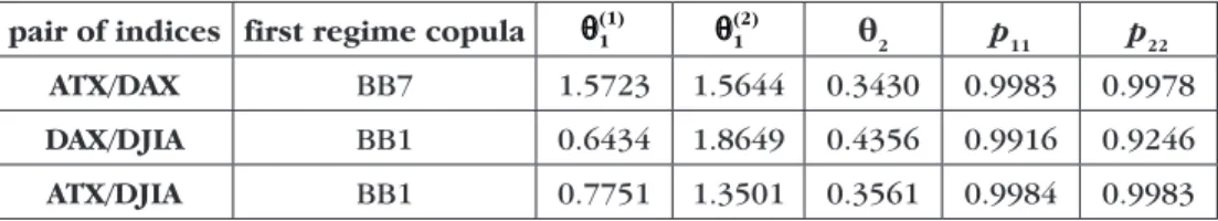
In the next step we estimated the regime switching copulas. To describe a dependence asymmetry we use two-parameter Archimedean copulas (BB1, BB4 and BB7) and Gaussian copula to model symmetric dependence with tail-independence patterns. In Table 7 we present the estimation results.
Table 7
Estimation results of regime switching copulas
pair of indices first regime copula T(1)1
(2) 1 T LJ2 p11 p22 ATX/DAX BB7 1.5723 1.5644 0.3430 0.9983 0.9978 DAX/DJIA BB1 0.6434 1.8649 0.4356 0.9916 0.9246 ATX/DJIA BB1 0.7751 1.3501 0.3561 0.9984 0.9983 Table 5 cont.
The optimal portfolio in respect to Expected Shortfall: a comparative study
All of the estimated parameters are significant. The copulas that fit the best are chosen using AIC and BIC information criterions. The correctness of the cop-ula specification are validated by an Anderson-Darling test applied to the first derivative of copulas: C u v| dC
du and |
dC C v u
dv.
In addition, based on estimated parameters of the transition matrix we com-puted the mean time of return to regimes. In all cases this value is lower for the asym-metric regime with a dependence in tails. For all pairs, the dependence between ex-tremely low returns is stronger than between exex-tremely high returns. The strength of dependence measured by weighted Kendall coefficients is the strongest for the DAX/ DJIA pair (with value 0.564) and the weakest for the ATX/DJIA pair (value 0.352).
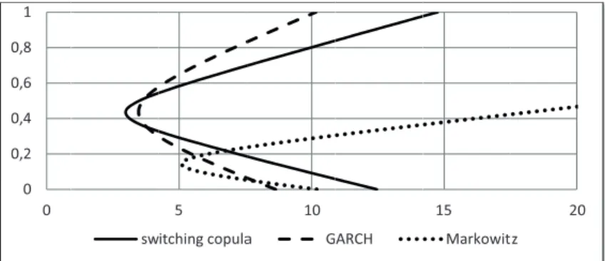
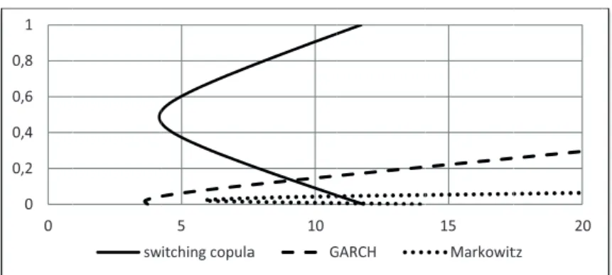
The standard method of visualization of measure of risk under the assumed model is drawing of the efficient frontier line. An efficient frontier for a given measure of risk is the curve showing the minimal risk of portfolio which exhibit the calculated expected returns.
For all three indices’ pairs and the two risk measures, Figures 1–6 illustrate simi-lar relationships. 0 0,2 0,4 0,6 0,8 1 0 sw 5 itchingcopula 10 a GARCH 15 Markowit 20 tz
Figure 1. Efficient frontiers of Value at Risk for ATX/DAX pair
0 0,2 0,4 0,6 0,8 1 0 sw 5 itchingcopula 10 a GARCH 15 Markowit 20 tz
0 0,2 0,4 0,6 0,8 1 0 sw 5 itchingcopula 10 a GARCH 15 Markowit 20 tz
Figure 3. Efficient frontiers of Value at Risk for ATX/DJIA pair
0 0,2 0,4 0,6 0,8 1 0 sw 5 itchingcopula 10 a GARCH 15 Markowit 20 tz
Figure 4. Efficient frontiers of Expected Shortfall for ATX/DJIA pair
0 0,2 0,4 0,6 0,8 1 0 sw 5 itchingcopula 10 a GARCHG 15 Markowit 20 tz
The optimal portfolio in respect to Expected Shortfall: a comparative study 0 0,2 0,4 0,6 0,8 1 0 sw 5 witchingcopula 10 a GGARCH 15 Markowit 20 tz
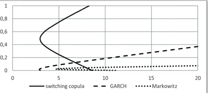
Figure 6. Efficient frontiers of Expected Shortfall for DAX/DJIA pair
Relatively small means of returns, presented in Table 2 cause a rapid increase of risk with increasing an expected portfolio return for the Markowitz model. Clearly, by definition, for every pair and every model ES is higher than VaR, see formula (33). Since negative expected returns are not interesting from a practical point of view, the included figures outline only the risks for positive expected returns.
For low expected returns (lower than 0.2 for ATX/DAX and ATX/DJIA pairs and lower than 0.05 for DAX/DJIA pair), the mean-variance model underestimates risks and after reaching some level overestimates them. The similar relation is observed for the GARCH model applied for the DAX/DJIA pair, but for the higher level. For ATX/DAX and ATX/DJIA pairs, the multivariate GARCH model underestimates risks for almost every level.
The level of an expected return, for which the minimum of a risk is attained, is determined by the forecast’s multidimensional mean. At this particular time, means of all the three indices are the lowest for the Markowitz model, means of ATX/DAX and ATX/DJIA pairs are at similar levels for the switching copula model and the GARCH model.
With increasing of the expected return, VaR and ES increase with the similar speed for models based on a normal distribution. However, for all three pairs, ES increases essentially faster than VaR in the case of copula based model. A positive tail dependence in switching copula models and relatively fat tails of marginal
dis-tributions, such as a skewed t distribution, are reasons for this observation.
7. Conclusions
Recent contributions suggest non-normal distributions of multivariate asset’s returns. Evidences for an asymmetry in univariate distributions and in dependences have been found. Furthermore, the kurtosis of an univariate distribution and
extreme dependences are found to be greater than under the assumption of nor-mal distribution. In the three analysed pairs of assets, all of these anonor-malies have been detected. Any model in which the conditional distribution is assumed to be normal does not fit since statistical tests reject hypothesis of normal distributions.
For the three pairs under study a switching copula models fit well. This model includes asymmetries and fat tails for both margins and for dependences. Conducted statistical tests confirmed goodness of fit for the switching copula models. Comparing results of a risk calculation, for the GARCH model and the Markowitz model to the switching copula model, we observed discrepancies.
A mean-variance model does not assume a dynamic structure of series, the expected mean of the series is significantly different for a dynamic model. Thus, a multivariate GARCH and a switching copula models forecast the mean at the similar level, while the estimated mean, using Markowitz model, stands out.
Misspecifications may cause both, an underestimation and an overestimation of a risk. Slopes of efficient frontiers describe the speed of increase of a risk with increasing expected return. It is observed that slopes for models which neglect anomalies, such as asymmetries and fat tails, are biased. In particular, a change of slope with the increasing expected return is underestimated.
Evaluations differ particularly for the Expected Shortfall risk. A tail’s de-pendences and fat tails are ignored in models based on a normal distribution. Expected Shortfall measures not only a frequency of a loss, but also its size. The supposition that observed anomalies of the multivariate distribution of an assets’ returns vector affects the size of an extreme return is confirmed.
References
[1] Aielli G., Consistent estimation of large scale dynamic conditional cor relations, University of Messina, Department of Economics, Statistics, Mathematics and Sociology, Working paper n. 47, 2008.
[2] Ang A., Bekaert G., ,QWHUQDWLRQDO DVVHW DOORFDWLRQ ZLWK UHJLPH VKLIWV, “Review of Financial Studies”, 2002, vol. 15(4), pp. 1137–1187.
[3] Ang A., Chen J., $V\PPHWULFFRUUHODWLRQVRIHTXLW\SRUWIROLRV, “Journal of Financial Economics” 2002, vol. 63(3), pp. 443–494.
[4] Artzner P., Delbaen F., Eber J., Heath D., Coherent Measures of Risk, “Mathematical Finance” 1999, vol. 9(3), pp. 203–228.
[5] Ball C.A., Torous W. N., Stochastic Correlation across International Stock
Markets, “Journal of Empirical Finance” 2000, vol. 7, pp. 373–388.
[6] Bekaert G., Wu G., Asymmetric Volatility and Risk in Equity Markets, “Review of Financial Studies” 2000, vol. 13, pp. 1–42.
The optimal portfolio in respect to Expected Shortfall: a comparative study
[7] Campbell R., Koedijk K., Kofman P., Increased Correlation in Bear Markets,
“Financial Ana lysts Journal” 2002, vol. 58, pp. 87–94.
[8] Chollette L., Heinen A., Valdesogo A., Modeling international financial re
WXUQVZLWKDPXOWLYDULDWHUHJLPHVZLWFKLQJFRSXOD, “Journal of Financial Econo metrics” 2009, vol. 7, pp. 437–480.
[9] Croux C., Joossens K., Robust estimation of the vector autoregressive mo
GHOE\DOHDVWWULPPHGVTXDUHVSURFHGXUH, in: Paula Brito (ed.), COMP-STAT 2008, pp. 489–501.
[10] Das S., Uppal R., ,QWHUQDWLRQDO3RUWIROLR&KRLFHZLWK6\VWHPLF5LVN, “Journal
of Finance” 2004, vol. 59 , pp. 2809–2834.
[11] Davison A.C., Smith R.L., Models for Exceedances over High Thresholds,
“Journal of the Royal Statistical Society” 1990, vol. 52, pp. 393–442.
[12] DiClemente A., Romano C., 0HDVXULQJSRUWIROLR9DOXHDW5LVNE\D&RSXOD
(97EDVHGDSSURDFK, “Studi Economici”2005, vol. 85,pp. 29–57.
[13] Embrechts P., McNeil A., Straumann D., &RUUHODWLRQ DQG 'HSHQGHQFH
3URSHUWLHV LQ 5LVN 0DQDJHPHQW 3URSHUWLHV DQG 3LWIDOOV, in: Risk Management: Value at Risk and Beyond, M. Dempster (eds), Cambridge, U.K.: Cambridge University Press, 2002, pp. 176–223.
[14] Erb C. B., Harvey C. R., Viskanta T. E., Forecasting International Correlation,
“Financial Analysts Journal” 1994, vol. 50, pp. 32–45.
[15] Fantazzini D., '\QDPLF FRSXOD PRGHOOLQJ IRU 9DOXH DW 5LVNFrontiers in
Finance and Economics 2008, vol. 31, pp. 161–180.
[16] Föllmer H., Schied A., Stochastic Finance: An Introduction in Descrete
Time, Walter de Gruyter, Berlin, 2011
[17] Guidolin M., Timmermann A., Term Structure of Risk under Alternative
(FRQRPHWULF 6SHFLILFDWLRQV, “Journal of Econometrics” 2006, vol. 131, pp. 285–308.
[18] Hamao Y., Masulis R.W., Ng V., Correlations in Price Changes and Volatility
across Interna tional Stock Markets, “Review of Financial Studies” 1990, vol. 3, pp. 281–308.
[19] Hamilton J.D., $QHZDSSURDFKWRWKHHFRQRPLFDQDO\VLVRIQRQVWDWLRQDU\
time series and the business cycle, “Econometrica” 1989, vol. 57, pp. 357–384.
[20] Hamilton J.D, Analysis of Time Series Subject to Changes in Regime, “Journal
of Econometrics” 1990, vol. 45, pp. 39–70.
[21] Junker M., May A., 0HDVXUHPHQW RI DJJUHJDWH ULVN ZLWK FRSXODV.
“Econometrics Journal” 2005, vol. 8, pp. 428–454.
[22] King M., Sentana E., Wadhwani S., 9RODWLOLW\DQG/LQNVEHWZHHQ1DWLRQDO
Stock Markets, “Econometrica” 1994, vol. 62, pp. 901–933.
[23] King M., Wadhwani S., 7UDQVPLVVLRQRI9RODWLOLW\EHWZHHQ6WRFN0DUNHWV
[24] Kole E., Koedijk K.C.G., Verbeek M., 6HOHFWLQJFRSXODVIRUULVNPDQDJH
ment, “Journal of Banking & Finance”2007, vol. 31, pp. 2405–2423. [25] Ledford A.W., Tawn J.A., 6WDWLVWLFVIRU1HDU,QGHSHQGHQFHLQ0XOWLYDULDWH
Extreme Values, “Biometrika” 1997, vol. 55 , pp. 169–187.
[26] Lin W., Engle R., Ito T., Do bulls and bears move across borders? International transmission of stock returns and volatility, “Review of Financial Studies”1994, vol.7(3), pp. 507–538.
[27] Longin F., Solnik B., Is the Correlation in International Equity Returns
&RQVWDQW" “Journal of International Money and Finance”1995, vol. 14, pp. 3–26.
[28] Longin F., Solnik B., Extreme Correlation of International Equity Markets, “Journal of Finance” 2001, vol. 56(2), pp. 649–676.
[29] Malevergne Y., Sornette D., 7HVWLQJWKH*DXVVLDQFRSXODK\SRWKHVLVIRUILQDQ
FLDODVVHWVGHSHQGHQFLHV, “Quantitative Finance”2003, vol. 3, pp. 231–250. [30] Markowitz H.M., Portfolio Selection: Efficient Diversification of Investments,
New York: John Wiley & Sons, 1959.
[31] Markwat T., Kole E., van Dijk D., 7LPHYDULDWLRQLQDVVHWUHWXUQGHSHQ
dence: Strength or structure?, Working paper, Erasmus University Rotterdam, 2010.
[32] Okimoto T., 1HZ (YLGHQFH RI $V\PPHWULF 'HSHQGHQFH 6WUXFWXUHV LQ
International Equity Markets, “Journal of Financial and Quantitative Analysis” 2008, vol. 43(3), pp. 787–815.
[33] Palaro H.P., Hotta L.K., 8VLQJFRQGLWLRQDOFRSXODWRHVWLPDWHYDOXHDWULVN
“Journal of Data Science” 2006,vol. 4, pp. 93–115.
[34] Patton A., 2Q WKH RXWRIVDPSOH LPSRUWDQFH RI VNHZQHVV DQG DV\PPH
WULFGHSHQGHQFHIRUDVVHWDOORFDWLRQ, “Journal of Financial Econometrics” 2004, vol. 2(1), pp. 130–168.
[35] Poon S.H., Rockinger M., Tawn J., ([WUHPH9DOXH'HSHQGHQFHLQ)LQDQFLDO
0DUNHWV 'LDJQRVWLFV 0RGHOV DQG )LQDQFLDO ,PSOLFDWLRQV, “Review of Financial Studies” 2006, vol. 17, pp. 581–610.
[36] Ramchand L., Susmel R., Volatility and cross correlation across major stock markets, “Journal of Empirical Finance” 1998, vol.17, pp. 581–610. [37] Rodriguez J., 0HDVXULQJILQDQFLDOFRQWDJLRQ$FRSXODDSSURDFK, “Journal
of Empirical Finance” 2007, vol.14, pp. 401–423.
[38] Weiß G.N.F., $UH &RSXOD*R)WHVWV RI DQ\ SUDFWLFDO XVH" (PSLULFDO HYL
dence for stocks, commodities and FX futures, “The Quarterly Review of Economics and Finance” 2011, vol. 51, pp. 173–188.