Uncertainty Modelling and Stability Robustness Analysis of Nucleic Acid-Based Feedback Control Systems

Uncertainty Modelling and Stability Robustness Analysis of Nucleic

Acid-Based Feedback Control Systems

Nuno M.G. Paulino

, Mathias Foo

, Jongmin Kim

and Declan Bates

Abstract— Recent advances in nucleic acid-based chem-istry have highlighted its potential for the implementation of biomolecular feedback circuits. Here, we focus on a proposed design framework, which is able to approximate the input-output behaviour of key linear operators used in feedback control circuits by combining three elementary chemical re-actions. The implementation of such circuits using DNA strand displacement introduces non-linear internal dynamics due to annihilation reactions among different molecular species. In addition, experimental implementation of in silico designs introduces significant levels of uncertainty and variability in reaction rate constants and equilibrium concentrations. Previ-ous work using this framework has overlooked the practical implications of these issues for the construction of nucleic acid-based feedback control circuits. Here, we analyse the impact of these nonlinearities and uncertainties on the stability of a biomolecular feedback loop. We show that a rigorous analysis of its nucleic acid-based implementation requires an investigation of the associated non-linear dynamics, to decide on realisable parameters and acceptable equilibrium concentrations. We also show how the level of experimental uncertainty that is tolerated by the feedback circuit can be quantified using the structured singular value. Our results constitute a first step towards the development of a rigorous robustness analysis framework for nucleic acid-based feedback control circuits.

I. INTRODUCTION

A primary aim of synthetic biology is the development of systematic design and analysis frameworks for biomolecular feedback control systems that can regulate concentrations of molecular species inside the cell [1]. The recently proposed use of chemical reaction networks (CRNs), implemented via nucleic acid-based chemistry, as a programming language for the design of such systems [2], has made it possible to conceptualise many biological circuits in line with classical feedback control ideas, [3], [4].

However, a direct translation of abstract mathematical operators (e.g. gain, summation) into biomolecular circuits via chemical reactions is often not straightforward. For example, implementation of the subtraction operator using CRNs generally results in a one-sided operation, (i.e. it can only compute a positive difference between two inputs), whereas in feedback control the error signal generated by

†N. Paulino and D. Bates are with the Warwick Integrative Syn-thetic Biology Centre (WISB), School of Engineering, University of War-wick, Coventry CV4 7AL, UK 1_{[email protected],} 4_{[email protected]}

2_{M. Foo is with the School of Mechanical, Aerospace and}

Automotive Engineering, Faculty of Engineering, Environment and Computing, Coventry University, Coventry CV1 5FB, UK [email protected]

3_{J. Kim is with the Wyss Institute for Biologically Inspired}

En-gineering, Harvard University, Boston, Massachusetts 02115, USA [email protected]

the difference between the measured and the desired values can take both positive and negative values. This is a critical limitation, as a one-sided error computation can lead to poor control performance or even instability [5], [6].

To get around this problem, Oishi and Klavins [3] pro-posed a formalism that can perform a two-sided subtraction, by letting each signal in the circuit be the difference in the concentration of two chemical species, x+ and x−. In this way, a systematic framework for implementing simple linear biomolecular feedback controllers can be developed using three elementary reactions, and the same formalism has recently been extended to include more complicated mathematical operators [7] and non-linear controllers [8], [9]. While previous studies have indicated satisfactory stability and performance properties for controllers designed using this framework, no formal robustness analysis of these circuits has so far been attempted. This is an important issue, because the implementation of CRNs using nucleic acids requires the matching of specified reaction rates for the required biomolecular reactions to realise a particular operator, which can be problematic in real experimental implementations.

The use of nucleic acids to implement CRNs is appealing because a simple kinetic model of toehold-mediated strand displacements could explain a large number of different strand displacement reactions from the DNA sequences [10]. However, predicting reaction rate constants from sequence information alone, i.e. without experimental inputs, is still challenging and can result in large deviations from pre-dicted design values. Improved biophysical models [11] and computational tools [12] can help improve the precision of predicted kinetics of hybridization and toehold-mediated strand displacement. It is also reasonable to assume that the different reactions may be characterised and the rates measured. Finally, varying the concentrations of auxiliary species [2] can also be used to iteratively bring the reaction rates closer to their design values. Based on the above considerations, it is estimated that environmental factors, together with uncertainty of the characterisation, i.e., the difference between measured rates and the actual reaction rates in the implementation, could result in uncertainty in the values of rate constants of between10% to20%.

Thus, it is crucial to be able to formally quantify in advance the robustness of proposed CRN-based designs to specified levels of uncertainty. Although some formal defi-nitions of robustness in systems biology have been proposed [13], the rigorous analysis of the effects of perturbations and uncertainties in synthetic circuits calls for more structured

2018 IEEE Conference on Decision and Control (CDC) Miami Beach, FL, USA, Dec. 17-19, 2018

𝐺(𝑠)

Δ

𝑢

𝑦

Fig. 1. Representation forµ-analysis, where the nominal linear system G(s)is interconnected with the uncertainty structured in the system∆.

mathematical formulations for robustness analysis, estima-tion and model-based predicestima-tion [14].

Here, we investigate the internal stability of the com-plete set of reactions resulting from an implementation of a linear feedback control circuit using nucleic acid-based chemistry. The assumption of high concentrations of inter-mediary species allows some simplification of the reactions, but still captures an important aspect missing from the input-output behaviour of the system: the circuit has non-linearities due to the annihilation reactions, which are not observable in the input-output dynamics. We show that the presence of these hidden internal dynamics has an impact on the equilibrium of the system, and also imposes lower bounds on the concentrations of the intermediary species. More importantly, the attraction of the equilibrium condition and its stabilising role also needs to be characterised. Secondly, we use the structured singular value (SSV) tool [15], [16] from robust control theory to perform a formal validation of the robustness of the proposed controller. An informal robustness and sensitivity analysis was carried out in [3], where the system was subjected to a square wave as reference input over 50 simulations in the presence of random±10% variability in the reaction rates. This led to mismatches in some of the reactions rates, causing significant steady state errors in the input tracking. In contrast to simulation-based approaches, the SSV analysis does not rely on statistics, making it a very strong certification method as long as the modelling of the underlying uncertainty is representative.

The use of SSV, orµ-analysis, has been previously inves-tigated in systems biology [17] in an attempt to quantify and validate robustness in natural biochemical networks [18], and it is now widely used in other domains such as aircraft [19], [20] and space engineering [21]. Once the uncertainty in the circuit is established, it can be aggregated in an uncertain system∆ interconnected with the nominal system (see Fig. 1), representing an infinite family of systems accounting for all possible combinations of the uncertain parameters, where any variation of the parameters will cause a deviation from the nominal response. The SSV analysis searches for the µ value (see e.g. [19]), which is a metric defining how far the system is from losing stability. If the domain of∆ does not contain destabilising parameter combinations, then robust stability is guaranteed for the specified level of uncertainty.

II. UNCERTAINTY MODELLING

Fig. 2 shows the configuration of the feedback control sys-tem analysed throughout this work. It is a

single-input/single-P

𝑘

_𝑃

𝑘

_𝐼

𝑠

+

𝜉

= 𝑥

+

_{− 𝑥}

𝑢

𝑦

-𝜉

= 𝑥

− 𝑥

𝜉

= 𝑥

_{− 𝑥}

Fig. 2. The analysed feedback loop with proportional-integral controller from [3].

output (SISO) system with a single stateξ4where the output

of a constant plantP = 1/(1 +%)tracks a reference inputu by the action of a proportional and integral controller. The closed-loop feedback trajectories evolve accordingly to:

˙

ξ4=kIξ1=kI(u−y) (1) y=P(kPξ1+ξ4)

A. CRN Approximation of a Linear Feedback Control Circuit Following the formalism introduced in [3], the configura-tion shown in Fig. 2 is approximated by a circuit composed of CRNs, where the negative and positive parts of a signal ξ are represented respectively by concentrations of two different speciesx+ _andx−_{. The final value of the signal is} retrieved withξ=x+_−x−_.

The proposed CRNs for each of the operations in the circuit are based on three elementary reactions, namely catal-ysis, annihilation and degradation. Here, the nomenclature x± represents compactly the two different species x+ _and x−. Similarly, the notationx± γ

±

−−→y± represents compactly two simultaneous reactions

x+ γ

+

−−→y+, x− γ −

−−→y− (2)

The element∅is used when the result of a reaction degrades, gets sequestered, or is removed, and no longer participates in the reactions.

Thus, the subtraction block ξ1 =u−ξ5 is approximated

by the reactions: u± γ ± 1 −−→u±+x±₁ , x±₅ γ ± 2 −−→x±₅ +x∓₁ (3) x±₁ γ ± 3 −−→ ∅ , x+₁ +x−₁ −→ ∅η

For the weighted integratorξ˙4=kIξ1, the CRNs are: x±₁ k

±

I

−−→x±₁ +x±₄ , x+₄ +x−₄ −→ ∅η (4) Finally, for the weighted summationy=ξ5=kpξ1+ξ4, we

have: x±₁ γ ± 7k ± P −−−−→x±₁ +x±₅ , x±₄ γ ± 8 −−→x±₄ +x±₅ (5) x±₅ γ ± 9(1+%) −−−−−→ ∅ , x+₅ +x−₅ −→ ∅η

The parameters γi, kP, kI, and η represent the rates of the

reactions, and%is a constant (set to%= 2as in [3]). Using the law of mass action, where the rate of a chemical reaction

is proportional to the product of the concentrations of the reactants (see e.g. [22]), the dynamics of the CRNs in (3)-(5) can be modelled using the ordinary differential equations (ODE): ˙ x+₁ =−γ₃+x+₁ +γ₂−x−₅ +γ₁+u+−ηx+₁x−₁ (6) ˙ x−₁ =−γ₃−x−₁ +γ₂+x+₅ +γ−₁u−−ηx+₁x−₁ (7) ˙ x+₄ =k+_Ix₁+−ηx+₄x−₄ (8) ˙ x−₄ =k−_Ix₁−−ηx+₄x−₄ (9) ˙ x+₅ =−γ₉+(1 +%)x+₅ +γ₇+k+_Px+₁ +γ₈+x+₄ −ηx+₅x−₅ (10) ˙ x−₅ =−γ₉−(1 +%)x−₅ +γ−₇k_P−x−₁ +γ₈−x₄−−ηx+₅x−₅ (11) The input-output systems have states computed by the dif-ference in concentration of the species tracking the positive and negative components of the signal withξi=x+i −x

−

i .

Considering the nominal case whereγ+_i =γ_i−, the dynamics of the CRNs are linear and are given by

˙ ξ=   −γ3 0 −γ2 kI 0 0 γ7kP γ8 −γ9(1 +%)  ξ+   γ1 0 0  u (12)

With the right choice of ratesγi, and controller parameters kI and kP, the input-output behaviour of (12) mimics the

input-output behaviour of the linear system shown in Fig. 2. In this sense, the abstract CRNs of (3)-(5) can implement a similar input-output response to the feedback system (1) with biomolecular reactions, albeit with the inclusion of extra dynamics.

B. Implementation with Nucleic Acids

The abstract CRNs given above can be implemented exper-imentally using DNA strand displacement (DSD) reactions [2],[3],[11]. The parameters γ_i±, k_I±, and k_P± in the CRNs are set as functions of nominal strand displacement ratesq±_i . The individual dependencies ofγ_i± onq±_i are inferred from the DSD implementation in [3], and set as

γ_i±=1 2q ± i Cmax, i∈ {1,2,3,7,8,9} (13) k_I±=1 2q ± 5Cmax, k±P = q±₇ q±₈ (14)

The scaling parameter Cmax results from the DSD

im-plementation of the feedback system in [3], which relies on bimolecular reactions mediated by intermediary auxil-iary species with initial concentrations given by Cmax. If Cmax x±i (t), the concentration of the auxiliary species

can be considered almost constant, and the set of reactions of the DSD network can be approximated by the unimolecular reactions of the CRNs in (3)-(5). Thus it is important to consider a set of parameters where the concentrations remain small with respect toCmax.

The annihilation reaction η depends on a maximum displacement rate qmax [2], and the DSD implementation

proposed in [3] results in the equivalency η =1

2qmax (15)

Ifη γi, the annihilation reaction keeps the concentrations x+_i and x−_i minimal without changing the transmission of the signal ξi [3]. Often this entails that for steady state, if ξi >0 then x+i ≈ξi andx−i ≈0. For ξi <0 we have the

inverse withx−_i ≈ξi andx+i ≈0.

C. Implications of Non-Linear Dynamics

While the CRN model provides a framework to approxi-mate the dynamics in (1) using concentrations of chemical species, when dealing with the DSD implementation it is important to note that the dynamics of ξi do not provide

a complete description of the system. For example, the requirement that x±_i (t) Cmax cannot be verified from

the input-output response alone, since the concentrations of xi are not observable in the statesξi, or y.

In addition, the stability and steady states of the sys-tem cannot be inferred from (12) alone, due to the ab-sence of the non-linear annihilation reactions. Consider the non-negative state vector of species concentrations x =

x+₁, x−₁, x+₄, x−₄, x+₅, x−₅T

∈ _R+

0. The system of ODE’s

in (6)-(11) can be represented compactly as

˙

x = Ax+Bu−ηg(x) (16)

The input vector u= [u+_{, u}−_]T _{contains both positive and} negative components of the reference input, and the linear part of the model is given by

A=         −γ₃+ 0 0 0 0 γ−₂ 0 −γ₃− 0 0 γ₂+ 0 k_I+ 0 0 0 0 0 0 k−_I 0 0 0 0 γ₇+k_P+ 0 γ₈+ 0 −γ₉+(1 +%) 0 0 γ₇−k−_P 0 γ−₈ 0 −γ₉−(1 +%)         B=        γ₁+ 0 0 γ₁− 0 0 0 0 0 0 0 0        , C= [ 0 0 0 0 1 −1 ]

A non-linear term g(x) is now present containing the multiplications due to bimolecular annihilation reactions:

g(x) =         x+₁x−₁ x+₁x−₁ x+4x − 4 x+₄x−₄ x+₅x−₅ x+₅x−₅        

As mentioned above, the statesξi∈Rare obtained from

the six non-negative componentsx±_i ∈R+0. This subtraction

results in the projection of the trajectories x±_i in a R3

manifold, defined by the projection matrixΨ :_R6_→

R3 Ψ =   1 −1 0 0 0 0 0 0 1 −1 0 0 0 0 0 0 1 −1   (17)

Applying this projection to the non-linear system in (16) we have thatΨ·g(x) = 0, and the trajectories ofξi result from

the linear dynamics

˙

ξ=Ψ(Ax+Bu−ηg(x)) = 1 2ΨAΨ

0 0.1 0.2 0.3 0.4 0.5 0.6 0.7 0.8 0.9 1 0.95 1 1.05 1.1 0 0.01 0.02 0.03 0.04 0.05 0.06 0.07 0.08

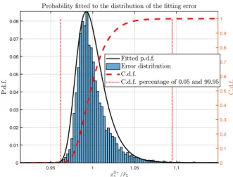
Fig. 3. Probability density function fitted to the distribution of the equilibrium estimation(1 +e6) = x0+₅ /ˆr5 (solid black), and the limits

(dotted red) containing 99.9% of the respective cumulative distribution function (dashed red).

An immediate consequence is that the steady state of (18) tells us nothing about the steady state of the DNA strand concentrations, which are the solution to (16).

The other significant consequence is that, in our example, while 1₂ΨAΨT _{is Hurwitz, the matrixAis not. The stability}

of the experimental implementation using DSD depends also on ηg(x) and the equilibrium solution. For example, with initial conditions x(0) = 0, at t = 0 the system in (16) is unstable (g(x) = 0 and A is not Hurwitz). The non-linear term ηg(x) is an adaptive stabilising term, where the state x needs to converge to an equilibrium where the system becomes stable. By collapsing the trajectories with the projection (17), this information about the internal stability is hidden.

D. Equilibria Change with Uncertainty on the Parameters Our objective is to measure the robustness of the system to uncertainty. The strand displacement ratesq_i± depend on the designed DNA toehold sequences [10], which can be hard to predict. Even after experimental characterisation, there will always be an error between the measured and real value of the reaction rates. Here, we consider that the reaction rates are never perfectly known and are therefore uncertainties in the system.

Considering the start of the time response to be when u+_=u−_{= 0, the equilibrium conditionx}0_{is the non-trivial}

solution to the non-linear equation

η·g(x0) =Ax0 (19) Thus the solution depends on the parametrisation of A and the strand displacement rates q_i±. Since it depends directly on the uncertain parameters, the solution is a moving equilibrium, [23], that changes with the values of the rates. However, through numerical simulation of the dynamics in (16) it is possible to produce an arbitrary number of pairs as-sociating an equilibrium conditionx0_{with the corresponding}

values ofq±_i , opening the way for estimation techniques. The SSV analysis framework requires rational representations of

uncertainty, and therefore each of the equilibrium compo-nents must be approximated by a polynomial function of the rates. To do this, the 14 uncertain ratesq_i± are organised in a column vectorq¯, and an estimator is obtained through the linear function

x0=r(¯q) +ε=Vq¯+ε (20)

The samples of x0 _{and q¯ are arranged respectively as}

columns of R and Q, and V = RQT _QQT−1

is the outcome of a Least Squares (LS) fitting. The fit of each of the components is further improved by expressing the LS fitting error εi, i ∈ {1, . . . ,6} as a quadratic function of ri(¯q): ˆ ri(¯q) =ri(¯q) + αi+βiri(¯q) +ρi(ri(¯q)) 2 +ϑi (21)

This new function reduces quadratic distortions of the errors and εi < ϑi. The fittings of the matrix V and the three

column vectorsα,β, andγ in (21) were done using 10000

random samples ofq_i± in the intervals in Table I, to arrive at the estimation function and error

x0(¯q) = ˆr(¯q)(1 +e) (22)

Despite the presence of a small estimation error, we have now computed a rational function that relates the uncertain parameters and the equilibrium state.

To account for the estimation error we add correspond-ing uncertainties, as suggested in [23], obtained from the distributions of the fitting errors for each component ei.

These were fitted with a probability density function (p.d.f.). Limits of variability for ei were defined containing 99.9%

of the cumulative density function to define six additional uncertainties, which cover the error in tracking the moving equilibria x0

i = ˆri(¯q) · δei. The resulting limits of all

uncertainties δei in the presence of 13% of uncertainty on q_i± are listed in Table I. See the case of error (1 +e5) in

Fig. 3 when estimating x0+₅ .

Linearising (16) around the equilibrium point (x, u) = (x0,0) then allows for a frequency representation of the system’s response around its equilibrium, which is suitable for analysis within the SSV framework. The error dynamics

TABLE I

UNCERTAIN SET∆COMPRISED BY THE REACTION RATESqiAND THE FITTING ERROR OF THE EQUILIBRIUMδei.

Name Nominal Variability

q_i±,i∈ {1,2,3,5,7,8,9} 800 [13,13] % δe1 1 [0.967081 1.09241] δe2 1 [0.967098 1.09217] δe3 1 [0.962463 1.06614] δe4 1 [0.962197 1.06822] δe5 1 [0.961924 1.09484] δe6 1 [0.96421 1.10709]

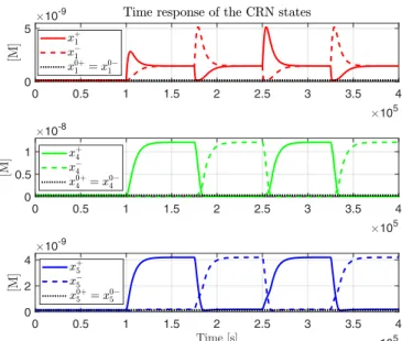
0 0.5 1 1.5 2 2.5 3 3.5 4 105 -5 0 5 10 -9 0 0.5 1 1.5 2 2.5 3 3.5 4 105 -5 0 5 10 -9

Fig. 4. Top: reference inputu = u+−u−and its two components. Bottom: output of the projected CRN in (18) (dashed black) approximates the response of the ideal linear model in (1) (blue).

around equilibrium x0 _are

˙ xe= ∂f ∂x _x0 xe+ ∂f ∂u _x0 ue = A−ηJ(x0) xe+Bue (23) ye=x+5e−x − 5e (24)

where xe =x−x0, ue =u−u0, and y = ye−y0. The

Jacobian matrixJ(x0_{)is given by} J(x0) = ∂g(x) ∂x _x0_,0 =         x0₁− x0+₁ 0 0 0 0 x0₁− x0+₁ 0 0 0 0 0 0 x0₄− x0+₄ 0 0 0 0 x0₄− x0+₄ 0 0 0 0 0 0 x0₅− x0+₅ 0 0 0 0 x0₅− x0+₅         (25)

The function in (22) is used to include ∆ in the Jacobian throughJ(ˆri(¯q)·δei)to account for the moving equilibrium

conditions. In this way, the equilibrium becomes correlated with the uncertainty, as in the original non-linear system. This step is important in order to remove the conservatism that would be introduced by assuming an independent vari-ability of the equilibrium conditions.

III. ANALYSIS RESULTS

The model in (16) for the non-linear system was imple-mented and simulated in Matlab/Simulinkr_{, and analysed} with the Robust Control Toolbox from Mathworks [24].

In our example,Cmax= 1µM and the displacement rates qi = 800M−1s−1 (as in [3]). The maximum rate was set

to qmax = 106M−1s−1. The reference input u(t) is given

by a square wave oscillating between ±4×10−9M. The desired alternating step input is composed of the difference between two concentrations in the presence of the annihila-tion reacannihila-tionu+_+u−_{−→ ∅}η _{(see Fig. 4). The trajectoriesx}±

i

for the complete nominal system in (16) are shown in Fig. 5

0 0.5 1 1.5 2 2.5 3 3.5 4 105 0 5 10-9 0 0.5 1 1.5 2 2.5 3 3.5 4 105 0 0.5 1 10-8 0 0.5 1 1.5 2 2.5 3 3.5 4 105 0 2 4 10-9

Fig. 5. Trajectories of the states for the non-linear system in (16), with initial conditions around the equilibrium solution of (19).

when the initial conditions are set tox0_{. The tracking error} ξ1=x+1−x

−

1 can assume positive and negative values and is

null at steady state. The trajectories ofx±₁ are not inferable fromξ1, wherex+1 andx

−

1 are always positive, and alternate

their role with each new step on the reference.

For the robustness analysis we consider that variability is present for all 14 strand displacement reaction rates independently, which can allow forq_i+ 6=q−_i . The nominal and uncertain values for q±_i and the fitting errors δei are

summarised in Table I. The final system has a high repetition of uncertainties, and for strictly real uncertainties it can be computationally hard to obtain good lower bounds on the SSV (= 1/µ). However, it is sufficient to demonstrate that the upper-bound of the SSV is less than 1 for all frequencies to guarantee that the system is stable for all possible parameterisations (see e.g. [19]).

As shown in Fig. 6, for uncertainty in the reaction rates of up to13%, the SSV analysis guarantees that the closed-loop system is stable for all uncertain parameters shown in Table I, since the upper bound on1/µ remains below1 for all frequencies. For levels of 14% or more the analysis is not conclusive. Since the fitting errorsδei introduce

conser-vatism, which does not exist in the non-linear system where the equilibrium is always the true value, a better description of rˆ(¯q) would improve the accuracy of the bound. Even with this extra artificial conservatism, however, our analysis shows that the system is guaranteed to be robustly stable for a13% variation in the reaction rates, which falls within the expected 10−20% level of experimental uncertainty. This represents crucial information to help experimentalists estimate the accuracy with which reaction rates need to be implemented for successful construction of these circuits.

IV. CONCLUSIONS

In this paper we investigated the problem of designing linear feedback control circuits that can be practically

im-10-7 10-6 10-5 10-4 10-3 10-2 0.5 1 1.5 13% 14% 15% 16% 17%

Fig. 6. Upper bounds on destabilising 1/µ, for different levels of uncertainty. The upper bounds are lower than1across all frequencies for uncertainty levels of13%or lower.

plemented using nucleic acid-based chemistry. We showed how the implementation of even simple linear circuits with distinct chemical species depends on non-linear terms that drive important dynamics which are not observable in the system’s input-output response. Rigorous analysis of the robustness of such circuits requires that we focus on the dynamics of the complete state vector and analyse the internal stability of the system. This provides information about closed loop stability and the system’s steady state that is highly relevant when choosing experimental parameters.

The use of the SSV framework provides a method for the rigorous quantification of how much the circuit implemen-tation deviates from the ideal response in the presence of experimental uncertainty, and allows a certification of the stability of the system around its equilibrium conditions. To achieve a linear representation, it was necessary to express the equilibrium conditions as a function of the uncertainty, to account for shifts due to parameter variability. We found the system to be robustly stable around its equilibrium for experimentally feasible uncertainty levels in the reaction rates. Further work is ongoing to investigate the significance of the non-linear terms in the dynamics of more complex feedback circuits, to improve the estimation of the moving equilibrium, to include additional sources of uncertainty, to quantify the effects of uncertainties on performance, and to obtain improved estimates of likely ranges of the uncertainties based on experimental data.

ACKNOWLEDGEMENT

Funding from the EPSRC & BBSRC (Centre for Doctoral Training in Synthetic Biology EP/L016494/1, and Warwick Integrative Synthetic Biology Centre BB/M017982/1).

REFERENCES

[1] D. Del Vecchio, A. J. Dy, and Y. Qian, “Control theory meets synthetic biology,”Journal of Royal Society Interface, vol. 13, no. 120, 2016.

[2] D. Soloveichik, G. Seelig, and E. Winfree, “DNA as a universal substrate for chemical kinetics,”Proceedings of the National Academy of Sciences, vol. 107, no. 12, pp. 5393–5398, 2010.

[3] K. Oishi and E. Klavins, “Biomolecular implementation of linear I/O systems,”IET Systems Biology, vol. 5, no. 4, pp. 252–260, 2011. [4] Y.-J. Chen, N. Dalchau, N. Srinivas, A. Phillips, L. Cardelli, D.

Solove-ichik, and G. Seelig, “Programmable chemical controllers made from DNA,”Nature Nanotechnology, vol. 8, no. 10, pp. 755–762, 2013. [5] M. Foo, J. Kim, J. Kim, and D. G. Bates, “Proportional-integral

degra-dation control allows accurate tracking of biomolecular concentrations with fewer chemical reactions,” IEEE Life Sciences Letters, vol. 2, no. 4, pp. 55–58, 2016.

[6] M. Foo, J. Kim, R. Sawlekar, and D. G. Bates, “Design of an embedded inverse-feedforward biomolecular tracking controller for enzymatic reaction processes,”Computers & Chemical Engineering, vol. 99, pp. 145 – 157, 2017.

[7] M. Foo, R. Sawlekar, J. Kim, D. G. Bates, G. B. Stan, and V. Kulkarni, “Biomolecular implementation of nonlinear system theoretic opera-tors,” inProc. European Control Conference, Aalborg, Denmark, Jun. 2016, pp. 1824–1831.

[8] R. Sawlekar, F. Montefusco, V. V. Kulkarni, and D. G. Bates, “Im-plementing nonlinear feedback controllers using DNA strand displace-ment reactions,”IEEE Transactions on NanoBioscience, vol. 15, no. 5, pp. 443–454, 2016.

[9] M. Foo, R. Sawlekar, and D. G. Bates, “Exploiting the dynamic properties of covalent modification cycle for the design of synthetic analog biomolecular circuitry,” Journal of Biological Engineering, vol. 10, no. 1, p. 15, 2016.

[10] D. Y. Zhang and E. Winfree, “Control of DNA strand displacement kinetics using toehold exchange,”Journal of the American Chemical Society, vol. 131, no. 47, pp. 17 303–17 314, 2009.

[11] N. Srinivas, T. E. Ouldridge, P. ˇSulc, J. M. Schaeffer, B. Yurke, A. A. Louis, J. P. K. Doye, and E. Winfree, “On the biophysics and kinetics of toehold-mediated DNA strand displacement,”Nucleic Acids Research, vol. 41, no. 22, pp. 10 641–10 658, 2013.

[12] J. X. Zhang, J. Z. Fang, W. Duan, L. R. Wu, A. W. Zhang, N. Dalchau, B. Yordanov, R. Petersen, A. Phillips, and D. Y. Zhang, “Predict-ing DNA hybridization kinetics from sequence,” Nature Chemistry, vol. 10, no. 1, pp. 91–98, 2018.

[13] S. Nikolov, E. Yankulova, O. Wolkenhauer, and V. Petrov, “Principal difference between stability and structural stability (robustness) as used in systems biology,”Nonlinear Dynamics, Psychology and Life Sciences, vol. 11, no. 4, pp. 413–433, 2007.

[14] S. Streif, K.-K. K. Kim, P. Rumschinski, M. Kishida, D. E. Shen, R. Findeisen, and R. D. Braatz, “Robustness analysis, prediction, and estimation for uncertain biochemical networks: an overview,”Journal of Process Control, vol. 42, pp. 14–34, 2016.

[15] P. M. Young, M. P. Newlin, and J. C. Doyle, “mu analysis with real parametric uncertainty,” inProc. 30th IEEE Conference on Decision and Control, Brighton, UK, Dec 1991, pp. 1251–1256.

[16] K. Zhou, J. C. Doyle, and K. Glover,Robust and optimal control. New Jersey: Prentice Hall, 1996.

[17] J. Kim, D. G. Bates, I. Postlethwaite, L. Ma, and P. A. Iglesias, “Ro-bustness analysis of biochemical network models,”IEE Proceedings -Systems Biology, vol. 153, no. 3, pp. 96–104, 2006.

[18] D. G. Bates and C. Cosentino, “Validation and invalidation of systems biology models using robustness analysis.” IET Systems Biology, vol. 5, no. 4, pp. 229–244, 2011.

[19] D. G. Bates and I. Postlethwaite,The Structured Singular Value and

µ-Analysis. Berlin, Heidelberg: Springer Berlin Heidelberg, 2002, pp. 37–55.

[20] G. Ferreres and J.-M. Biannic, “Reliable computation of the robustness margin for a flexible aircraft,”Control Engineering Practice, vol. 9, no. 12, pp. 1267 – 1278, 2001.

[21] J. Doyle, K. Lenz, and A. Packard, “Design examples using µ-synthesis: Space shuttle lateral axis FCS during reentry,” inProc. IEEE Conference on Decision and Control, Athens, Greece, Dec. 1986, pp. 2218–2223.

[22] B. Ingalls,Mathematical Modeling in Systems Biology: An Introduc-tion, ser. Mathematical Modeling in Systems Biology. Cambridge, MA: MIT Press, 2013.

[23] L. Andersson and A. Rantzer, “Robustness of equilibria in nonlinear systems,”IFAC Proceedings Volumes, vol. 32, no. 2, pp. 2256 – 2261, 1999.