Dynamic Compensation Based Control of a
Comprehensive Model of Wheeled Mobile Robots
Zhang Xu
1, Li Jie
2, Zhang Wei
2,*1School of Mechanical Engineering, Beijing Institute of Technology, Beijing, China 2Department of Electrical Engineering, Beijing Institute of Technology, Beijing, China
Copyright©2016 by authors, all rights reserved. Authors agree that this article remains permanently open access under the terms of the Creative Commons Attribution License 4.0 International License
Abstract
This paper uses the general framework of dynamic feedback linearization for stabilization of mobile robots. Instead of using unicycle model for control design, this paper uses a comprehensive model which is based on the physics of differential drive robots. The model used in the paper describes nonholonomic underactuated behavior of robot in terms of the physical dimensions and velocities of the wheels. Next, the proposed control is applied to this model and it is theoretically proven that dynamic feedback linearization can successfully solve the stabilization problem. To evaluate the performance of proposed control, another controller is designed based on the Lyapunov’s method. The performance of the two controllers and the complexity of control gain tuning process are compared. Next, the robustness of the proposed control against uncertainties is studied. The results of analysis and simulations show that the proposed control has very good performance against parametric uncertainties.Keywords
Mobile Robots, Posture Stabilization, Differential Drive Robots, Dynamic Compensation, Lyapunov Based Control Design1. Introduction
Mobile robots are used for many applications [1] which range from service robotics [2] to mapping and surveillance applications [3], rescue robotics [4] and management of disastrous situations [5,6]. Fairly simple mechanism of work of mobile robots makes them a popular class of robots for such applications. Differential drive robots (DDR) are a class of mobile robots with two active wheels on the sides of the robot. The third wheel in the structure of robot is the caster wheel which is responsible for providing counter weight balancing forces through the ground reaction. The difference in the angular velocities of the wheels determines direction of motion of robot. There are theoretically challenging issues involved in the control of differential drive robots and
several interesting control problems have been studied for DDRs. Tracking control, path following and regulation of the posture of DDRs are the mostly studied control problems.
DDRs are nonholonomic systems since the rolling without slipping constraint describing the kinematics of their motion is not integrable. Also, the number of control inputs for the system is less than the number of states. Therefore, DDRs are classified within the category of underactuated nonholonomic systems. Stabilization of these robots is challenging and cannot be achieved by smooth, time invariant control strategies. Many research groups have used discontinuous controls [8-10] to solve this fundamental challenge. Using feedback linearization based approaches [7, 11, 12] has also been very successful for stabilization of DDRs. Motivated by the fact that a stabilizing controller cannot be smooth and time invariant, time varying controls [13-15] have also been widely used for posture regulations problem. In addition to the basic problem, posture stabilization problem have also been studied for multi-robot scenarios where the robot is towing one or several trailers [16, 18]. Input constrained posture stabilization where hard limits are posed on the magnitude of the control inputs have also been studied [19, 20]. In addition to the kinematic model of differential drive robots, several studies have focused on controlling the full dynamics of DDRs [21, 22] as well. Similar to posture stabilization, tracking control of differential drive robots is also widely studied [23-26]. Fuzzy logic controllers have been a commonly used tool for this purpose [27, 28]. Adaptive [29,30] and robust control [31,32] methods have also been successfully used to improve the performance of tracking controllers against uncertainties and disturbances.
of robust controls for stabilization of differential drive robots. This paper shows the success of dynamic feedback linearization approach in stabilizing the posture of robot via analytical proof and simulation results. Also, to verify the performance of the proposed control strategy, another control is designed for the comprehensive model. The performance and ease of tuning of the two controllers are compared. The results of simulations show that the dynamic feedback linearization based control has a smoother stabilization path and easier tuning process. Finally, the performance of the proposed controller is studied under parametric uncertainties. The results of the simulations show that the proposed control has a very good performance against uncertainties.
2. Modeling Mobile Robots
A vast majority of the papers in the literature use the unicycle model for designing controls for differential drive robots. In this section, we review the unicycle model of differential drive robots and then proceed to derive a new comprehensive model for this class of mobile robots which closely models the physics of their motion under the assumption of rolling without slipping. We finally study the properties of the developed model.
2.1. Unicycle Model of Differential Drive Robots
Unicycle model is the model of a disc rolling on a 2D surface under the assumption of rolling without slipping. This model is usually shown as a driftless nonlinear system with the following form:
�𝑦̇𝑥̇ 𝛽̇�=�
𝑐𝑜𝑠𝛽 0
𝑠𝑖𝑛𝛽 0
0 1� �𝑣𝜔� (1)
where x and y represent the coordinates of the robot and β denotes the heading of the robot. In this model the control inputs, v and 𝜔 denote the forward velocity of the robot and its rotation rate. However, this is a very abstract model focused on describing the rolling without slip phenomena.
2.2. The Proposed Comprehensive Model for Differential Drive Robots
In this paper, we will develop a more comprehensive model for differential drive robots which incorporates the physical dimensions of the system into the model. Consider the schematics of a general differential drive robot in Fig. 1 where β is the heading of the robot. Velocities of the centres of left and right wheels can be found as below by taking derivative of the corresponding position vectors:
𝑉𝐿=��𝑋̇ − 𝐿𝛽̇𝑐𝑜𝑠𝛽�𝑠𝑖𝑛𝛽 − �𝑌̇ − 𝐿𝛽̇𝑠𝑖𝑛𝛽�𝑐𝑜𝑠𝛽�𝑒1(2)
+��𝑋̇ − 𝐿𝛽̇𝑐𝑜𝑠𝛽�𝑐𝑜𝑠𝛽+�𝑌̇ − 𝐿𝛽̇𝑠𝑖𝑛𝛽�𝑠𝑖𝑛𝛽�𝑒2
𝑉𝑅=��𝑋̇+𝐿𝛽̇𝑐𝑜𝑠𝛽�𝑠𝑖𝑛𝛽 − �𝑌̇+𝐿𝛽̇𝑠𝑖𝑛𝛽�𝑐𝑜𝑠𝛽�𝑒1(3)
+��𝑋̇+𝐿𝛽̇𝑐𝑜𝑠𝛽�𝑐𝑜𝑠𝛽+�𝑌̇+𝐿𝛽̇𝑠𝑖𝑛𝛽�𝑠𝑖𝑛𝛽�𝑒2 where X and Y denote the position of the point between the wheels of the robot and e1, e2 is a moving coordinate frame on the robot where e1 is in the direction of main axle of the robot and e2 is on the wheel axis. The kinematic model of the system can be found by imposing zero relative velocity between the ground and the contact points of the wheels with the ground. Finding the velocity of the contact points using equations (2) and setting the velocity components in e1 and e2 directions to zero yields:
�𝑋̇ − 𝐿𝛽̇𝑐𝑜𝑠𝛽�𝑠𝑖𝑛𝛽 − �𝑌̇ − 𝐿𝛽̇𝑠𝑖𝑛𝛽�𝑐𝑜𝑠𝛽= 0 (4) �𝑋̇ − 𝐿𝛽̇𝑐𝑜𝑠𝛽�𝑐𝑜𝑠𝛽+�𝑌̇ − 𝐿𝛽̇𝑠𝑖𝑛𝛽�𝑠𝑖𝑛𝛽 − 𝑟𝜑̇𝐿= 0(5) where 𝜑̇𝐿,𝑟 denote the angular velocities of the left wheel of the robot and the radius of the wheel respectively. Substituting equation (4) into (5) and after algebraic manipulations, the following equation can be found:
[image:2.595.326.536.322.611.2]𝑌̇ − 𝐿𝛽̇𝑠𝑖𝑛𝛽=𝑟𝜑̇𝐿𝑠𝑖𝑛𝛽 (6)
Figure 1. Schematics of the differential drive robot
Following the same procedure for the velocity of the right wheel in (4), the following equation is achieved:
𝑋̇+𝐿𝛽̇𝑐𝑜𝑠𝛽=𝑟𝜑̇𝑅𝑐𝑜𝑠𝛽 (7) where 𝜑̇𝑅 denote the angular velocities of the left wheel. Finally, the last equation can be found by applying the relative velocity formula between the two contact points of the wheels with the ground:
The kinematics of the differential drive robot under the assumption of rolling without slipping can be represented by equation (6-8) which can be shown in matrix form as:
�1 00 1 −𝐿𝑠𝑖𝑛𝛽𝐿𝑐𝑜𝑠𝛽
0 0 𝑑 � � 𝑋̇ 𝑌̇ 𝛽̇�=�
0 𝑟𝑐𝑜𝑠𝛽
𝑟𝑠𝑖𝑛𝛽 0
−𝑟 𝑟 � �𝜑̇
𝐿 𝜑̇𝑅� (9)
2.3. Model Properties
Similar to the unicycle model, this model describes a set of nonholonomic constraints as expected. To verify this, equation (9) is rephrased and expressed as a driftless system:
𝑞̇ ≜ �𝑋̇𝑌̇
𝛽̇�=𝑔1(𝑞)𝜑̇𝐿+𝑔2(𝑞)𝜑̇𝑅 (10) where:
𝑔1(𝑞) =
⎣ ⎢ ⎢ ⎢ ⎢ ⎡ 𝑟𝐿𝑐𝑜𝑠𝛽 𝑑 𝑟𝑠𝑖𝑛𝛽 −𝑟𝐿𝑠𝑖𝑛𝛽𝑑
−𝑑𝑟 ⎦⎥ ⎥ ⎥ ⎥ ⎤
,𝑔2(𝑞) =
⎣ ⎢ ⎢ ⎢ ⎢
⎡𝑟𝑐𝑜𝑠𝛽 −𝑟𝐿𝑐𝑜𝑠𝛽𝑑 𝑟𝐿𝑠𝑖𝑛𝛽
𝑑 𝑟
𝑑 ⎦⎥
⎥ ⎥ ⎥ ⎤
Therefore, the kinematic model of system is fully non-holonomic since the distribution Δ=𝑠𝑝𝑎𝑛{𝑔1,𝑔2} is not involutive:
𝑅𝑎𝑛𝑘(𝑔1,𝑔2, [𝑔1𝑔2]) = 2 <𝑑𝑖𝑚 (𝑞) (11) where [. , . ] denotes the Lie bracket operator.
3. Controller Design via Dynamic
Feedback Linearization
Similar to standard static feedback linearization, the final goal of dynamic feedback linearization is achieving a linear system from the perspective of system input-output. Unlike conventional feedback linearization that state feedback in used, linearization is achieved by using the so called dynamic state in dynamic feedback linearization approach. The conditions of achieving full state linearization via dynamic feedback linearization are less strict and are satisfied for a larger class of non-holonomic systems including wheeled mobile robots that are transformable into chained form.
3.1. General Formulation
The dynamic feedback linearization problem is formulated as below [7,8]. Given a general nonlinear system:
Σ: 𝑥̇=𝑓(𝑥) +𝑔(𝑥)𝑢 (12) where 𝑥 ∈ ℝ𝑛 and 𝑢 ∈ ℝ𝑚, find a dynamic compensator:
𝒞: �𝑢=𝛼(𝑥,𝜉) +𝛽(𝑥,ξ)𝑣
𝜉̇=𝛾(𝑥,𝜉) +𝛿(𝑥,𝜉)𝑣 (13) such that the closed-loop system (12), (13) is equivalent to a linear system under the transformation 𝑧=𝜙(𝑥,𝜉).
Existence of such a dynamic compensator and the linearizability of the system are directly related to existence of a linearizing output and flatness of the system. Necessary conditions, sufficient condition (but not necessary and sufficient) have been developed for existence of such a dynamic compensator. Fortunately, it has been shown that mobile robot models which can be transformed into chained form are linearizable in the dynamic feedback linearization sense.
3.2. Posture Stabilization Control Design
To design a posture stabilizing control for our model of differential drive robots (9), a two stage design procedure has been used. First a dynamic feedback linearization control is designed and then a stabilizing control is designed for the linearized system. The final control is discontinuous at the origin as predicted by Brockett’s conditions. Theorem I defines the dynamic feedback based linearizing control and proves its linearizing property.
Theorem I: Consider the rolling without slipping kinematic of the differential drive robots in (9). Defining the state transformation as:
𝑧=�𝑧𝑧1
2�=�𝑋𝑌� (14) the dynamic compensator defined by:
𝜉̇=𝑣1𝑐𝑜𝑠𝛽+𝑣2𝑠𝑖𝑛𝛽, 𝜉(0) =𝜉0
�𝜑̇𝐿 𝜑̇𝑅�=�
𝜉 𝑟−
𝑑
2𝑟𝜉(𝑣2𝑐𝑜𝑠𝛽 − 𝑣1𝑠𝑖𝑛𝛽) 𝜉
𝑟+ 𝑑
2𝑟𝜉(𝑣2𝑐𝑜𝑠𝛽 − 𝑣1𝑠𝑖𝑛𝛽)
� (15)
linearizes the kinematic model (1).
Proof: Substituting (15) into the kinematic model (9), we have:
�1 00 1 −𝐿𝑠𝑖𝑛𝛽𝐿𝑐𝑜𝑠𝛽
0 0 𝑑 � �
𝑋̇ 𝑌̇ 𝛽̇�=
⎣ ⎢ ⎢ ⎢
⎡𝜉𝑐𝑜𝑠𝛽+2𝑑𝜉𝑐𝑜𝑠𝛽(𝑣2𝑐𝑜𝑠𝛽 − 𝑣1𝑠𝑖𝑛𝛽)
𝜉𝑠𝑖𝑛𝛽 −2𝑑𝜉𝑠𝑖𝑛𝛽(𝑣2𝑐𝑜𝑠𝛽 − 𝑣1𝑠𝑖𝑛𝛽)
𝑑
𝜉(𝑣2𝑐𝑜𝑠𝛽 − 𝑣1𝑠𝑖𝑛𝛽) ⎦ ⎥ ⎥ ⎥ ⎤
(16) Taking the inverse of the upper triangular matrix on the left hand side and defining the linearizing output as 𝜂= (𝑋,𝑌)′, algebraic simplifications yield:
𝜂̇=�𝑋̇
𝑌̇�=�𝜉𝑐𝑜𝑠𝛽𝜉𝑠𝑖𝑛𝛽� (17) Taking derivative of both sides of (17) and considering the fact that 𝑧1=𝑋,𝑧2=𝑌:
�𝑧𝑧1̈
2̈ �=�𝑋̈𝑌̈�=�𝜉
̇𝑐𝑜𝑠𝛽 − 𝜉𝛽̇𝑠𝑖𝑛𝛽
where according to (8):
𝛽̇=𝑟𝑑(𝜑̇𝑅− 𝜑̇𝐿) (19) 𝛽̇=1
𝜉(𝑣2𝑐𝑜𝑠𝛽 − 𝑣1𝑠𝑖𝑛𝛽) Substituting (15) and (19) into (18):
�𝑧𝑧1̈ 2̈ �=�
(𝑣1𝑐𝑜𝑠𝛽+𝑣2𝑠𝑖𝑛𝛽)𝑐𝑜𝑠𝛽 −(𝑣2𝑐𝑜𝑠𝛽 − 𝑣1𝑠𝑖𝑛𝛽)𝑠𝑖𝑛𝛽
(𝑣1𝑐𝑜𝑠𝛽+𝑣2𝑠𝑖𝑛𝛽)𝑠𝑖𝑛𝛽+ (𝑣2𝑐𝑜𝑠𝛽 − 𝑣1𝑠𝑖𝑛𝛽)𝑐𝑜𝑠𝛽�(20)
�𝑧1̈ 𝑧2̈ �=�
𝑣1 𝑣2�
which completes the proof.
It is worth mentioning that the choice of the output is based on the expected desired behavior of the system. Having chosen the linearizing output candidate, the dynamic extension algorithm is used to build up the dynamic compensator. If the obtained system is invertible from the chosen output, the algorithm terminates and the full input-state-output linearization is achieved.
The next step is designing the linear control on the linearized system to achieve the stabilization. In fact, the overall control is the combination of a linear control and the dynamic feedback based linearizing control. Theorem II introduces this stabilizing control for the linearized system.
Theorem II [8]: Consider the rolling without slipping kinematic of the differential drive robots in (9) under the action of dynamic compensator (15). The following PD control:
𝑣=�𝑣𝑣12�=�𝑘𝑝1 𝑘𝑝2� �𝑋𝑌�+ [𝑘𝑑1 𝑘𝑑2]�𝑋𝑌̇̇� (21) guarantees exponential convergence to the origin from any initial configuration if:
𝑘𝑑21−4𝑘𝑝1=𝑘𝑑22−4𝑘𝑝2> 0
𝑘𝑑2− 𝑘𝑑1> 2�𝑘𝑑22−4𝑘𝑝2 (22)
𝜉0≠2
𝑘𝑝1𝑋0𝑠𝑖𝑛𝛽0− 𝑘𝑝1𝑌0𝑐𝑜𝑠𝜃0 𝑘𝑑2− 𝑘𝑑1
[image:4.595.64.293.598.699.2]where 𝑋0,𝑌0,𝛽0 denote the initial configuration of the robot.For the proof, the reader is referred to [8].
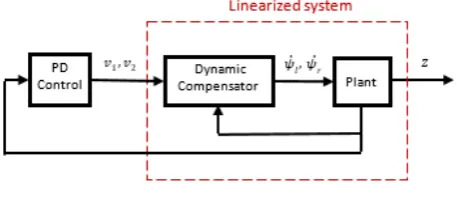
Figure 1. Control System Structure
Therefore, the overall control structure is comprised of two control loops, the inner loop linearizes the system with the aid of a dynamic compensator and the outer loop
stabilizes the linearized system. Figure 2 demonstrates this control idea via a graphic schematics:
4. Control Design via Lyapunov’s
Technique
To verify the performance of the stabilizing controller proposed in this paper, another stabilizing control is designed for the comprehensive model in (9). This controller is based on Lyapunov’s technique. Using Lyapunov analysis for the design of controllers is a common and effective approach for nonlinear systems. The idea is using a positive definite function and devising the control signals such that the time derivative of the function along the system trajectories is negative definite. To apply this idea to the problem of posture stabilization, we need to express the model of the system in Polar coordinates. Let’s consider the following change of variables:
�𝑅=√𝑋 2+𝑌2 𝛼=𝜃 − 𝛽+𝜋
𝛿=𝜃+𝜋
(23)
where θ is defined using the four quadrant tangent invers as: 𝜃=𝐴𝑇𝐴𝑁2(𝑌,𝑋)
Based on (23), the set of state equations can be rewritten in terms of the new state variables. To achieve this, the time
derivative of R and δ should be found using the original state equations:
𝑅̇= (𝑋𝑋̇+𝑌𝑌̇)
√𝑋2+𝑌2
� (24)
The time derivative terms in (24) can be found from the original state equations of the system (9) through algebraic manipulations:
⎩ ⎪ ⎨ ⎪
⎧𝑋̇=�𝑟� �2 (𝜑̇𝐿+𝜑̇𝑅)𝑐𝑜𝑠𝜙 𝑌̇=�𝑟� �2 (𝜑̇𝐿+𝜑̇𝑅)𝑠𝑖𝑛𝜙
𝛽̇=− �𝑑�𝑟 (𝜑̇𝐿− 𝜑̇𝑅) Thus (24) can be rewritten as:
𝑅̇=�𝑟� �2 (𝜑̇𝐿+𝜑̇𝑅)�(𝑋𝑐𝑜𝑠𝜙+𝑌𝑠𝑖𝑛𝜙�𝑋2+𝑌2 )� (25)
There are certain geometric relationships between the parameters of the system. These relations can be easily deduced from Fig. 1:
� 𝑋
�𝑋2+𝑌2=𝑐𝑜𝑠𝜃=−𝑐𝑜𝑠𝛿
𝑌
�𝑋2+𝑌2=𝑠𝑖𝑛𝜃=−𝑠𝑖𝑛𝛿
(26)
Thus, (25) can be simplified to:
𝑅̇=−�𝑟� �2 (𝜑̇𝐿+𝜑̇𝑅)𝑐𝑜𝑠(𝛿 − 𝜙 (27)
follows:
𝛿̇=𝜃̇=�𝑟� �2 (𝜑̇𝐿+𝜑̇𝑅)𝑠𝑖𝑛(𝑅𝛿−𝜙) (28) The state equations of the transformed system can be written as:
⎩ ⎪ ⎨ ⎪
⎧𝑅̇=−�𝑟� �2 (𝜑̇𝐿+𝜑̇𝑅)𝑐𝑜𝑠(𝛿 − 𝜙) 𝛿̇=�𝑟� �2 (𝜑̇𝐿+𝜑̇𝑅)sin(𝛿−𝜙𝑅 )
𝜙̇=−�𝑟 𝑑� �(𝜑̇𝐿+𝜑̇𝑅)
(29)
Defining 𝛼=𝛿 − 𝜙, the equations of motion in (29) can be written as:
⎩ ⎪ ⎨ ⎪
⎧ 𝑅̇=− �𝑟2�(𝜑̇𝐿+𝜑̇𝑅)𝑐𝑜𝑠𝛼 𝛼̇=�𝑟2�(𝜑̇𝐿+𝜑̇𝑅)𝑠𝑖𝑛 𝛼𝑅 +�𝑟𝑑�(𝜑̇𝐿− 𝜑̇𝑅)
𝜙̇=− �𝑑𝑟�(𝜑̇𝐿− 𝜑̇𝑅)
(30)
Using the transformed system in (30), Lyapunov-based control design is used for synthesizing a posture stabilizing control. This procedure is outlined in Theorem III.
Theorem III: Consider the kinematic model of the differential drive robots in (30). Under the control laws:
�𝜑̇𝐿= 𝛾
𝑟𝑅𝑐𝑜𝑠𝛼 − 𝑑
2𝑟�𝑘𝛼+ 0.5 𝑠𝑖𝑛2𝛼
𝛼 (𝛼+ℎ𝛿)� 𝜑̇𝑅=𝛾𝑟𝑅𝑐𝑜𝑠𝛼+2𝑟𝑑�𝑘𝛼+ 0.5𝑠𝑖𝑛2𝛼𝛼 (𝛼+ℎ𝛿)�
(31)
where k, λ, and h are positive scalars, the differential drive robot is asymptotically stabilized.
Proof: The proof is by applying the direct Lyapunov method. Consider the following positive definite Lyapunov candidate function:
𝑉=12𝜆𝑅2+1
2(𝛼2+ℎ𝛿2) (32) As defined in (23), R is the norm of the distance from origin. Similarly, the second term in (32) is the norm of the alignment error. The time derivative of this positive definite function can be easily found to be:
𝑉̇=𝜆𝑅𝑅̇+𝛼𝛼̇+ℎ𝛿𝛿̇ (33) Substituting for the derivative of the state variables from (30), the time derivative of V along system trajectories is found as:
𝑉̇=−𝜆𝑅 �𝑟2�(𝜑̇𝐿+𝜑̇𝑅)𝑐𝑜𝑠(𝛿 − 𝜙) +𝛼 ��𝑟2�(𝜑̇𝐿+ 𝜑̇𝑅)𝑠𝑖𝑛(𝛿−𝜙𝑅 )+�𝑟𝑑�(𝜑̇𝐿− 𝜑̇𝑅)�+ℎ𝛿 ��𝑟2�(𝜑̇𝐿+ 𝜑̇𝑅)𝑠𝑖𝑛(𝛿−𝜙𝑅 )� (34) Next, the proposed control signals in (31) are substituted in (34). Using algebraic calculations and several simplifications via trigonometric identities, it can be shown that:
𝑉̇=−𝜆𝛾𝑅2𝑐𝑜𝑠2𝛼 − 𝜆(𝛾 𝑐𝑜𝑠2𝛼)𝑒2− 𝑘𝛼 (35) Equation (35) is negative semidefinite and thus the
Lyapunov analysis is inconclusive. Since the Lyapunov function V is positive definite, it is lower bounded by zero. On the other hand, as (35) shows the derivative of V is negative or zero and therefore V is a non-increasing function. Based on the two previous statements it can be inferred that the value of V converges asymptotically toward a finite non-negative value. Since V is a radially unbounded function, the state trajectories for any initially bounded condition will remain bounded which equivalently means 𝑉̇ is uniformly continuous in time. Based on Barbalat’s Lemma, 𝑉̇ converges to zero which means that the state of system will converge to [0, 0, 𝜃�] for some 𝜃�. The next step is showing that 𝜃� = 0 is the only possible solution. To show this, the closed-loop equations of the system is studied by substituting (31) into (30). The closed-loop system is:
�
𝑅̇=−𝜆𝑅 𝑐𝑜𝑠2𝛼 𝛼̇=−𝑘𝛼 −0.5 𝛾ℎ𝑠𝑖𝑛2𝛼𝛼
𝜃̇ =𝛾𝑐𝑜𝑠𝛼𝑠𝑖𝑛𝛼
(36)
It has been shown that the first and third equations converge to zero. The second differential equation in (36) implies that 𝛼̇ is converging to a finite limit value. Since it has been shown that state trajectories are bounded, thus 𝛼̇ is a uniformly continuous function in time. Therefore according to Barbalat’s lemma, 𝛼̇ converges to zero which implies that θ converges to zero. Therefore 𝜃�= 0 and the system is asymptotically stabilized to origin.
5. Simulation Results
To verify the performance of the stabilizing controller proposed in this paper, simulation results are provided in this section. The physical parameters of the differential drive robot used for simulation are r = 0.1 m and d = 2L = 0.3m. The first posture stabilization scenario considered here is as follows:
𝑞0=�1,2,−𝜋� �4 ′, 𝑞𝑓= (0, 0, 0)′
where q0 and qf denote the initial and final configurations of the robot. The initial condition of the 𝜉 parameter of the dynamic compensator is chosen as 𝜉0=−0.4 to realize the backward steering. The gains of the PD control are also chosen as:
𝑘𝑑2=−3,𝑘𝑑1=−8,𝑘𝑝1=−2,𝑘𝑝2=−14
The results of the simulation are given next. Figure 3 shows the path of the robot during the posture stabilization where black arrows show the robot axle. Fig. 4 shows the time evolution of the state variables and as shown in this figure, all the states are stabilized.
Figure 3. Robot Path during Stabilization
[image:6.595.154.458.76.747.2]Figure 4. Trajectories of the States of System
Figure 6. Robot Path during Stabilization - Lyapunov based Control
[image:7.595.150.455.72.755.2]Figure 7. Trajectories of the State of System - Lyapunov based Control
Figure 9. State Trajectories under Parameter Uncertainty - Dynamic Feedback linearization based Control
We aimed to compare the performance of the devised control with other methods. To this end, we have simulated the same stabilization scenario with the Lyapunov based control in (31). Figures 6 through 8 show the robot stabilization path, state trajectories and the corresponding control signals respectively under the Lyapunov based control.
As the figures show, the path of the dynamic feedback linearization based control is smoother. Also, the magnitude of the control signals in the case of dynamic feedback linearization is much smaller than the Lyapunov based control. Therefore, dynamic feedback linearization based control excels the Lyapunov based control performance wise in this simulation scenario.
Another aspect for evaluation of the performance of a controller is to study the robustness of the controller. Robustness of the controller can be measured against external disturbances and un-modeled dynamics which can be represented as the parametric and non-parametric uncertainties. In this paper, we focus on studying the effect of parametric uncertainty on the performance of the proposed controller. To study the effect of the parameter uncertainty on the performance of the stabilizing controller, the same posture stabilization scenario is simulated where a 20% parametric uncertainty has been added on the dimensions of the robot. In other words, the estimates of the parameters of the system used by the controller are: 𝑟̂= 0.12𝑚 ,𝑑̂= 0.24𝑚. In the case of dynamic feedback linearization based control, the parametric uncertainty will appear as an additive term after the feedback linearization. The results of the simulations show that the performance of the controller is robust to this level of uncertainty. However, the transient performance of the system is adversely affected and the oscillations of the state trajectories have increased.
To get an idea of how much uncertainty can be compensated, we keep increasing the magnitude of uncertainty to get to a point at which the controller fails. The interesting observation is that the controller is not sensitive to uncertainty in the d parameter and it can handle even large
uncertainties. On the other hand for the simulation scenario considered above, the controller is robust to uncertainties up to 45% in r parameter which is still very impressive. However, beyond this value stabilization errors appear in the final robot heading. For example figure 9 shows the stabilization trajectories for a 48% uncertainty, i.e. 𝑟̂= 0.148𝑚:
It is interesting to note that the two of the states are stabilized but the third state which is the unactuated degree of freedom in the underactuated does not converge to zero. This is due to the large magnitude of the nonlinear terms that has not been cancelled by the feedback linearization process. For future work, it is interesting to study the robustness issue in more depth and understanding why the sensitivity of the control is different for different system parameters. There should be an underlying reason which makes a certain parameter to be robust to uncertainties. Moreover, it is interesting to study the bounds for parameter estimation errors that would result in losing stability analytically.
6. Conclusions
in this paper. Simulation results are also provided that compare the performance of the proposed control with other controllers.
REFERENCES
[1] B. Siciliano, L. Sciavicco, L. Villani, and G. Oriolo, Robotics: Modelling, Planning and Control: Springer Publishing Company, Incorporated, 2008
[2] K. Watanabe, Y. Shiraishi, S. G. Tzafestas, J. Tang, and T. Fukuda, "Feedback Control of an Omnidirectional Autonomous Platform for Mobile Service Robots," Journal of Intelligent and Robotic Systems, vol. 22, pp. 315-330, 1998. [3] N. Ruangpayoongsak, H. Roth and J. Chudoba, Mobile robots
for search and rescue, IEEE International Safety, Security and Rescue Rototics, Workshop, 2005, 212-217.
[4] S. Hirose and E. F. Fukushima, "Development of mobile robots for rescue operations," Advanced Robotics, vol. 16, pp. 509-512, 2002/01/01 2002.
[5] H.-B. Kuntze, C. W. Frey, I. Tchouchenkov, B. Staehle, E. Rome, K. Pfeiffer, et al., "SENEKA-sensor network with mobile robots for disaster management," in Homeland Security (HST), 2012 IEEE Conference on Technologies for, 2012, pp. 406-410.
[6] H.-B. Kuntze, C. Frey, T. Emter, J. Petereit, I. Tchouchenkov, T. Mueller, et al., "Situation Responsive Networking of Mobile Robots for Disaster Management," in ISR/Robotik 2014; 41st International Symposium on Robotics; Proceedings of, 2014, pp. 1-8.
[7] G. Oriolo, A. D. Luca, and M. Vendittelli, "WMR control via dynamic feedback linearization: design, implementation, and experimental validation," IEEE Transactions on Control Systems Technology, vol. 10, pp. 835-852, 2002.
[8] A. Astolfi, "Exponential Stabilization of a Wheeled Mobile Robot via Discontinuous Control," Jour. of Dyn. Sys, Measurement, and Control, vol. 121, pp. 121-126, 1999. [9] O. Sørdalen and O. Egeland, "Exponential stabilization of
nonholonomic chained systems," Automatic Control, IEEE Transactions on, vol. 40, pp. 35-49, 1995.
[10]A. Zeiaee, R. Soltani-Zarrin, S. Jayasuriya, and R. Langari, A Uniform Control for Tracking and Point Stabilization of Differential Drive Robots Subject to Hard Input Constraints, ASME 2015 Dynamic Systems and Control Conference, V001T04A005-V001T04A005, 2015
[11]B. d'Andrea-Novel, G. Bastin, and G. Campion, "Dynamic feedback linearization of nonholonomic wheeled mobile robots," in Robotics and Automation, 1992. Proceedings., 1992 IEEE International Conference on, 1992, pp. 2527-2532. [12]K. Shojaei, A. M. Shahri, and A. Tarakameh, "Adaptive
feedback linearizing control of nonholonomic wheeled mobile robots in presence of parametric and nonparametric uncertainties," Robotics and Computer-Integrated Manufactur ing, vol. 27, pp. 194-204, 2011.
[13]P. Morin and C. Samson, "Application of backstepping
techniques to the time-varying exponential stabilisation of chained form systems," European journal of control, vol. 3, pp. 15-36, 1997.
[14]C. Samson, "Control of chained systems application to path following and time-varying point-stabilization of mobile robots," IEEE Transactions on Automatic Control, vol. 40, pp. 64-77, 1995.
[15]K. Shojaei and A. Shahri, "Adaptive robust time-varying control of uncertain non-holonomic robotic systems," IET Control Theory & Applications, vol. 6, pp. 90-102, 2012. [16]A. K. Khalaji and S. A. A. Moosavian, "Adaptive sliding mode
control of a wheeled mobile robot towing a trailer," Proceedings of the Institution of Mechanical Engineers, Part I: Journal of Systems and Control Engineering, vol. 229, pp. 169-183, 2015.
[17]A. K. Khalaji and S. A. A. Moosavian, "Stabilization of a tractor-trailer wheeled robot," Journal of Mechanical Science and Technology, vol. 30, pp. 421-428, 2016.
[18]A. K. Khalaji and S. A. A. Moosavian, "Dynamic modeling and tracking control of a car with n trailers," Multibody System Dynamics, vol. 37, pp. 211-225, 2016.
[19]R. Soltani-Zarrin, A. Zeiaee, and S. Jayasuriya, Pointwise Angle Minimization: A Method for Guiding Wheeled Robots Based on Constrained Directions, ASME 2014 Dynamic Systems and Control Conference, V003T48A004-V003T48A 004, 2014
[20]K. Shojaei, "Saturated output feedback control of uncertain nonholonomic wheeled mobile robots," Robotica, vol. 33, pp. 87-105, 2015.
[21]R. Soltani-Zarrin and S. Jayasuriya, Constrained directions as a path planning algorithm for mobile robots under slip and actuator limitations, 2014 IEEE/RSJ International Conference on Intelligent Robots and Systems, 2395-2400, 2014
[22]K. Shojaei, A. Mohammad Shahri, and A. Tarakameh, "Adaptive feedback linearizing control of nonholonomic wheeled mobile robots in presence of parametric and nonparametric uncertainties," Robotics and Computer-Integra ted Manufacturing, vol. 27, pp. 194-204, 2//2011.
[23]Z.-P. Jiang and H. Nijmeijer, "A recursive technique for tracking control of nonholonomic systems in chained form," IEEE Transactions on Automatic control, vol. 44, pp. 265-279, 1999.
[24]W. E. Dixon, D. M. Dawson, F. Zhang, and E. Zergeroglu, "Global exponential tracking control of a mobile robot system via a PE condition," IEEE Transactions on Systems, Man, and Cybernetics, Part B (Cybernetics), vol. 30, pp. 129-142, 2000. [25]M. Rahimi Bidgoli, A. Keymasi Khalaji, and S. A. A.
Moosavian, "Trajectory tracking control of a wheeled mobile robot by a non-model-based control algorithm using PD-action filtered errors," Modares Mechanical Engineering, vol. 14, 2015.
[26]A. Zeiaee, R. Soltani-Zarrin, and R. Langari, A novel approach for tracking control of differential drive robots subject to hard input constraints, American Control Conference, 2098-2103, 2016
robots," Asian Journal of Control, vol. 14, pp. 960-973, 2012. [28]Almeshal, Abdullah M., Mohammad R. Alenezi, and
Muhammad Moaz. "Intelligent Path Tracking Hybrid Fuzzy Controller for a Unicycle-Type Differential Drive Robot." World Academy of Science, Engineering and Technology, International Journal of Computer, Electrical, Automation, Control and Information Engineering, 901-904, 2015
[29]K. Shojaei, A. M. Shahri, A. Tarakameh, and B. Tabibian, "Adaptive trajectory tracking control of a differential drive wheeled mobile robot," Robotica, vol. 29, pp. 391-402, 2011.
[30]A. Keymasi Khalaji and S. A. A. Moosavian, "Adaptive sliding mode control of a wheeled mobile robot towing a trailer," Proceedings of the Institution of Mechanical Engineers, Part I: Journal of Systems and Control Engineering, vol. 229, pp. 169-183, 2015.
[31]A. Keymasi Khalaji and S. A. A. Moosavian, "Robust adaptive controller for a tractor–trailer mobile robot," Mechatronics, IEEE/ASME Transactions on, vol. 19, pp. 943-953, 2014. [32]Y. Jong-Min and K. Jong-Hwan, "Sliding mode control for