International Journal of Emerging Technology and Advanced Engineering
Website: www.ijetae.com (ISSN 2250-2459, Volume 2, Issue 10, October 2012)231
EFFICIENT AND FAST CLUSTERING ALGORITHM
FOR REAL TIME DATA
N.K. Sharma
1, Dr. R.C. Jain
2, Manoj Yadav
31 Assistant Professor,Ujjain Engineering College, Ujjain, M.P., India 2 Director, S.A.T.I. Engineering College, Vidisha, M.P., India
3 Software Consultant P.I.S.T. Bhopal, M.P., India
Abstract - Data mining is a powerful and new method of analyzing data and finding out new patterns from large set of data. The objective of data mining is to pull out knowledge from a data set in an understandable format. Data mining is the process of collecting, extracting and analyzing large data set from different perspectives.
Actually it is the analysis of large amount of data to squirm out existing interesting patterns to faction up similar data subsets i.e. cluster analysis along with dependencies (association rule mining). In this piece of work, an effort is laid down to calculate distance between formed clusters of data. Now, novelty of the work starts where bit-wise comparison and masking of clusters have been done over Java, which helps to accomplish the result more efficiently and rapidly.
The simulation of this approach is expounded and evaluated over data set of counseling for admission in various professional courses and in which clustering of dataset on the basis of allotment is done over and effectiveness is evaluated in terms of the time taken for the clustering process and purity (i.e. accuracy) of cluster is calculated which is a simple and transparent criteria for evaluation of accuracy for cluster.
Keywords – Data Mining, Clustering, Bit-wise Operator
I. INTRODUCTION
Clustering is a tool for analysis of data which in turns solves classification problems. Its objective is to distribute cases into groups, so that the degree of association becomes strong among members of the same clusters and weak among members of different clusters [1],[2]. In this way cluster describes classes for the different data sets. Clustering may reveal associations and structure in dataset which, was existing and useful, once found. The results of cluster analysis may contribute to the definition of a formal classification scheme, such as a taxonomy for related animals, insects or plants; or suggest statistical models with which to describe populations; or indicate rules for assigning new cases to classes for identification and diagnostic purposes; or provide measures of definition, size and change in what previously were only broad concepts; or find exemplars to represent classes[7]. In any kind of business, one needs to face with classification problem at some point of time. Cluster analysis might provide the methodology to help you to solve it.
Cluster analysis or clustering is the task of assigning a set of objects into groups (called clusters) so that the objects in the same cluster are more similar (in some sense or another) to each other than to those in other clusters. Clustering is a main task of explorative data mining, and a common technique for statistical data analysis used in many fields, including machine learning, pattern recognition, image analysis, information retrieval, and bioinformatics.
Cluster analysis itself is not one specific algorithm, but the general task to be solved. It can be achieved by various algorithms that differ significantly in their notion of what constitutes a cluster and how to efficiently find them. Popular notions of clusters include groups with low distances among the cluster members, dense areas of the data space, intervals or particular statistical distributions. The appropriate clustering algorithm and parameter settings (including values such as the distance function to use, a density threshold or the number of expected clusters) depend on the individual data set and intended use of the results. Cluster analysis as such is not an automatic task, but an iterative process of knowledge discovery that involves try and failure. It will often be necessary to modify preprocessing and parameters until the result achieves the desired properties.
II. CLUSTERING ALGORITHMS
Clustering algorithms can be categorized based on their cluster model. The following overview will only list the most prominent examples of clustering algorithm. Not all provide models for their clusters and can thus not easily be categorized [3],[4],[5].
A. Connectivity based clustering (Hierarchical clustering)
Connectivity based clustering, also known as hierarchical clustering, is based on the core idea of objects being more related to nearby objects than to objects farther away. As such, these algorithms connect "objects" to form "clusters" based on their distance.
Raw Data Clustering Algorithm
International Journal of Emerging Technology and Advanced Engineering
Website: www.ijetae.com (ISSN 2250-2459, Volume 2, Issue 10, October 2012)232
A cluster can be described largely by the maximum distance needed to connect parts of the cluster. At different distances, different clusters will form, which can be represented using a dendrogram, which explains where the common name "hierarchical clustering" comes from. These algorithms do not provide a single partitioning of the data set, but instead provide an extensive hierarchy of clusters that merge with each other at certain distances. In a dendrogram, the y-axis marks the distance at which the clusters merge, while the objects are placed along the x-axis such that the clusters don't mix.Connectivity based clustering is a whole family of methods that differ by the way distances are computed. Apart from the usual choice of distance functions, the user also needs to decide on the linkage criterion (since a cluster consists of multiple object, there are multiple candidates to compute the distance to) to use. Popular choices are known as single-linkage clustering (the minimum of object distances), complete linkage clustering (the maximum of object distances) or UPGMA ("Unweighted Pair Group Method with Arithmetic Mean", also known as average linkage clustering). Furthermore, hierarchical clustering can be computed agglomerative (starting with single elements and aggregating them into clusters) or divisive (starting with the complete data set and dividing it into partitions).
While these methods are fairly easy to understand, the results are not always easy to use, as they will not produce a unique partitioning of the data set, but a hierarchy the user still needs to choose appropriate clusters from. The methods are not very robust towards outliers, which will either show up as additional clusters or even cause other clusters to merge (known as "chaining phenomenon", in particular with single-linkage clustering). In the general case, the complexity is, which makes them too slow for large data sets. For some special cases, optimal efficient methods (of complexity) are known: SLINK for single-linkage and CLINK for complete-linkage clustering. In the data mining community these methods are recognized as a theoretical foundation of cluster analysis, but often considered obsolete. They did however provide inspiration for many later methods such as density based clustering.
B. Centroid-based Clustering
In centroid-based clustering, clusters are represented by a central vector, which must not necessarily be a member of the data set. When the number of clusters is fixed to k, k-means clustering gives a formal definition as an optimization problem: find the k cluster centers and assign the objects to the nearest cluster center, such that the squared distances from the cluster are minimized.
The optimization problem itself is known to be NP-hard, and thus the common approach is to search only for approximate solutions.
A particularly well known approximate method is Lloyd's algorithm,[3] often actually referred to as "k-means algorithms". It does however only find a local optimum, and is commonly run multiple times with different random initializations. Variations of k-means often include such optimizations as choosing the best of multiple runs, but also restricting the centroids to members of the data set (k-medoids), choosing medians (k-medians clustering), choosing the initial centers less randomly (K-means++) or allowing a fuzzy cluster assignment (Fuzzy c-means).
Most k-means-type algorithms require the number of clusters - k - to be specified in advance, which is considered to be one of the biggest drawbacks of these algorithms. Furthermore, the algorithms prefer clusters of approximately similar size, as they will always assign an object to the nearest centroid. This often leads to incorrectly cut borders in between of clusters (which is not surprising, as the algorithm optimized cluster centers, not cluster borders).
K-means has a number of interesting theoretical properties. On one hand, it partitions the data space into a structure known as Voronoi diagram. On the other hand, it is conceptually close to nearest neighbor classification and as such popular in machine learning. Third, it can be seen as a variation of model based classification, and Lloyd's algorithm as a variation of the Expectation-maximization algorithm for this model discussed below. C. K-Means Clustering Algorithm
This nonhierarchical method initially takes the number of components of the population equal to the final required number of clusters. In this step itself the final required number of clusters is chosen such that the points are mutually farthest apart. Next, it examines each component in the population and assigns it to one of the clusters depending on the minimum distance. The centroid's position is recalculated every time a component is added to the cluster and this continues until all the components are grouped into the final required number of clusters.
The k-means algorithm works as follows:
a) Randomly select k data object from dataset D as initial cluster centers.
b) Repeat
i. Calculate the distance between each data object
di(1<=i<=n) and all k cluster centers
cj(1<=j<=n) and assign data object di to the nearest
cluster.
ii. For each cluster j(1<=j<=k), recalculate the cluster
center.
iii.Until no changing in the center of clusters. The most
International Journal of Emerging Technology and Advanced Engineering
Website: www.ijetae.com (ISSN 2250-2459, Volume 2, Issue 10, October 2012)233
D. Distribution-based ClusteringThe clustering model most closely related to statistics is based on distribution models. Clusters can then easily be defined as objects belonging most likely to the same distribution. A nice property of this approach is that this closely resembles the way artificial data sets are generated: by sampling random objects from a distribution.
While the theoretical foundation of these methods is excellent, they suffer from one key problem known as overfitting, unless constraints are put on the model complexity. A more complex model will usually always be able to explain the data better, which makes choosing the appropriate model complexity inherently difficult.
The most prominent method is known as expectation-maximization algorithm. Here, the data set is usually modeled with a fixed (to avoid overfitting) number of Gaussian distributions that are initialized randomly and whose parameters are iteratively optimized to fit better to the data set. This will converge to a local optimum, so multiple runs may produce different results.
Distribution-based clustering is a semantically strong method, as it not only provides you with clusters, but also produces complex models for the clusters that can also capture correlation and dependence of attributes. However, using these algorithms puts an extra burden on the user: to choose appropriate data models to optimize, and for many real data sets, there may be no mathematical model available the algorithm is able to optimize (e.g. assuming Gaussian distributions is a rather strong assumption on the data).
E. Density-based Clustering
In density-based clustering, clusters are defined as areas of higher density than the remainder of the data set. Objects in these sparse areas - that are required to separate clusters - are usually considered to be noise and border points.
The most popular density based clustering method is DBSCAN. In contrast to many newer methods, it features
a well-defined cluster model called
"density-reachability". Similar to linkage based clustering; it is based on connecting points within certain distance thresholds. However, it only connects points that satisfy a density criterion, in the original variant defined as a minimum number of other objects within this radius. A cluster consists of all density-connected objects (which can form a cluster of an arbitrary shape, in contrast to many other methods) plus all objects that are within these objects range.
Another interesting property of DBSCAN is that its complexity is fairly low - it requires a linear number of range queries on the database - and that it will discover essentially the same results (it is deterministic for core and noise points, but not for border points) in each run, therefore there is no need to run it multiple times.
The key drawback of DBSCAN is that it expect some kind of density drop to detect cluster borders.
F. Graph-based approaches
To address the problem of clustering, k nearest neighbors (kNNs) are used to identify k most similar points around each point and by way of conditional merging, clusters are generated. There are various variants of kNN clustering and they differ at the conditional merging part of the solution. For a given point p, its kNNs are found out. If the distance between p and any of the points in kNN(p) set (say q) is less than ϵ, then point q is merged into the cluster of p. This algorithm requires tuning of ϵ and k values to get clusters. In a method proposed, to construct strongly connected components from a given directed graph where each edge is associated with a weight (usually distance between points). This method is highly sensitive to the presence of noise and cannot handle clusters of different densities.
III. PROPOSED WORK
Proposed algorithm is based on K-means algorithms [6],[7]. Actual Data base is used to calculate the distance between clusters. Binary comparator is used for comparison of clusters.
A. Proposed Algorithm Pre process data
Step 1: Read a record and convert its categorical value into binary value (i.e. 0 for Y, 1 for N).
Step 2: Merge these binary value into a single variable by masking and shifting.
Step 3: Choice is encode into code and store into an integer variable
Step 4: Create a Data point and add to array Step 5: if more record exist go to step 1. Step 6: Return array of Data points Check similar
B. Assumption & Calculations
Following are the assumptions of information used for the purpose and are tabulated below
TABLE 1: CASTE
Description Numerical Value Binary Value “UR” 0 00 “OBC” 1 01 “SC” 2 10 “ST” 3 11
TABLE 2: BELOW POWERTY LINE Description Numerical Value Binary Value
N 0 0
International Journal of Emerging Technology and Advanced Engineering
Website: www.ijetae.com (ISSN 2250-2459, Volume 2, Issue 10, October 2012)234
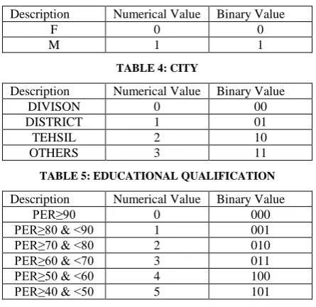
TABLE 3: GENDER
Description Numerical Value Binary Value
F 0 0
[image:4.595.53.276.148.364.2]M 1 1
TABLE 4: CITY
Description Numerical Value Binary Value DIVISON 0 00 DISTRICT 1 01 TEHSIL 2 10 OTHERS 3 11 TABLE 5: EDUCATIONAL QUALIFICATION Description Numerical Value Binary Value
PER≥90 0 000 PER≥80 & <90 1 001 PER≥70 & <80 2 010 PER≥60 & <70 3 011 PER≥50 & <60 4 100 PER≥40 & <50 5 101
[image:4.595.327.549.316.738.2]Now, based on these assumptions we will mask a 15 bit string which portrays all information as follows:
TABLE 6: 15 BIT STRING 1
5 1 4
1 3
1 2
1 1
1 0
9 8 7 6 5 4 3 2 1 0
CA
S
T
E
BP
L
GEN
DER
CITY
P
ERCE
NTA
GE
Now, as shown above, for information provided in tabular forms in each case can be encoded in to binary values. If suppose up to “n” information is to be
represented in binary form, then it will require “log2n”
number of binary bits, and then a 15 bit string is represented, each bit of which will represent an information in binary form. Hence, such strings are used for calculation of distance (or similarity) among them. More the similarity more will be the probability of being in same cluster. After normalizing the input data set and forming a string for an input record, masking between these strings is done to obtain similarity among them as follows:
Comparision using bit wise operator
(1) Y Y Y X11 X12 Y Y Y Y 0 0 0 1 1 0 0 0 0 (2) Y Y Y X21 X22 Y Y Y Y
Now, after formation of cluster, the effectiveness is checked by calculating purity of clusters, which is an external criterion for evaluation of accuracy.
To compute purity, each cluster is assigned to the class which is most frequent in the cluster, and then accuracy of this assignment is measured by counting the number of correctly assigned documents and dividing it by the total number of records. Mathematically,
Where Cu represents the k number of clusters formed, and cl represents the set of j number of classes with N number of total classes in clusters.
IV. DATABASE USED
TABLE 7: CHOICES FILLED
RollNo Pref
order
ccode inst_name branch Dist
name
400005 114 BBB Indore EC Indore
400005 212 BBB Indore EI Indore
400005 313 BBB Indore EE Indore
400005 417 BBB Indore MECH Indore
400005 510 BBB Indore CE Indore
400005 658 FFF INDORE ET Indore
400005 757 FFF INDORE EI Indore
400008 1 17 BBB Indore MECH Indore
400008 2 11 BBB Indore CSE Indore
400008 3 13 BBB Indore EE Indore
400008 4 14 BBB Indore EC Indore
400008 5 60 FFF INDORE MECH Indore
400008 6 56 FFF INDORE CSE Indore
400008 7 16 BBB Indore IT Indore
400008 8 12 BBB Indore EI Indore
400008 9 10 BBB Indore CE Indore
400008 1058 FFF INDORE ET Indore
400009 114 BBB Indore EC Indore
400009 211 BBB Indore CSE Indore
400009 317 BBB Indore MECH Indore
400009 416 BBB Indore IT Indore
400009 521 CCC Jabalpur EC Jabalpur
400009 624 CCC Jabalpur MECH Jabalpur
400009 719 CCC Jabalpur CSE Jabalpur
400009 823 CCC Jabalpur IT Jabalpur
400009 958 FFF INDORE ET Indore
400011 114 BBB Indore EC Indore
400011 213 BBB Indore EE Indore
[image:4.595.42.287.396.496.2]International Journal of Emerging Technology and Advanced Engineering
Website: www.ijetae.com (ISSN 2250-2459, Volume 2, Issue 10, October 2012)235
V. SIMULATION & RESULTS
Above explained approach is simulated over JAVA Run:
Category
UR: 5193 OBC: 3273 SC: 1148 ST: 386 BPL
N: 9985 Y: 15
[image:5.595.155.442.227.655.2]
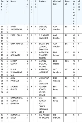
TABLE 8: ALLOTMENT MADE
Gender
F: 2506 M: 7494 City
Division: 4322 District: 1864 Block: 453 Out of State: 3361
Percentage
A: 78 B: 1147 C: 2681 D: 3349 E: 2156 F: 526 G: 63 Choice-1 DP: 10000 Ro ll N o M e r i t
Name C
a t c l a s s d o m i
Address Allotted
Inst Bran ch A ll o t e d c a t all ot ed cls 44 90 21 1 2 5 ARPIT SRIVASTAVA U R
X N JALAUN, KONCH
AAA Gwalior
EE U
R X 44 40 14 1 0 6
EKTA LODHI O
B C
S Y D D NAGAR
GWALIOR AAA Gwalior
EE O
B C S 45 11 92 1 1 1
UMA MAHOR S
C
X Y LAXMI BAI COLONY, GWALIOR
AAA Gwalior
EC S
C X 47 10 27 1 4 2 PRIYA AGRAWAL U R
X Y AGRAWAL
BHAWAN, INDORE
BBB Indore
CSE U
R X 47 11 61 1 4 1 SHRIYA GUPTA U R
X Y ANAND BAZAAR, INDORE
BBB Indore
CSE U
R X 48 01 47 1 0 5 RUCHI VISHWAKAR MA O B C
X Y HATHITAL, JABALPUR
CCC Jabalpur
CE O
B C X 44 85 58 6 9 AJAY PARIHAR S C
X Y MOHANGA
DH, GWALIOR
DDD Vidisha
EI S
C X 46 01 66 1 0 6 SACHIN GUPTA U R
X Y ADARSH
SCHOOL KE PAS, DAMOH
EEE Rewa
CE U
R X 51 59 79 1 0 4 KAMLENDRA KUMAR GAUTAM U R
X Y VILL KUWAN POST OFFICE JHALWAR, SIDHI EEE Rewa
CE U
R X 43 18 02 7 2 HEMLATA UIKEY S T
X Y B.N.P.COLO NY DEWAS
FFF INDORE
IT S
International Journal of Emerging Technology and Advanced Engineering
Website: www.ijetae.com (ISSN 2250-2459, Volume 2, Issue 10, October 2012)236
TABLE 9: CLUSTER FORMAION
CLUSTERS RECORDS TOTAL
RECORDS
Cluster0 4 5 13 … 117 121 4298
Cluster1 2 3 10 … 190 198 2289
Cluster2 1 6 7 … 43 44 1843
Cluster3 8 25 26 … 101 102 1570
Above table is an illustration of records clustered in specified clusters.
VI. CONCLUSION
The present work is carried in the general context of clustering algorithm which is based on bit wise comparison of the masked 15 bit string by calculating distance between them. The only difference, observed here is of better time complexity as compare to other counterparts along with accuracy of cluster formation. The new clustering algorithm proposed which is using a bit wise comparator on real time data used for admission in various engineering institutions. This algorithm helps one to assess his/her possibility of allotment of institutions of their choice on the basis of marks, caste, educational qualifications and location etc. the same can be improved when approached with other clustering techniques.
REFERENCES
[1 ] Masahiro Motoyoshi, Takao Miura, and Isamu Shioya, “Clustering by Regression Analysis”, LNCS 2737, 2003. [2 ] Matthew Gebski and Raymond K. Wong, “A New Approach for
Cluster Detection for Large Datasets with High Dimensionality”, Springer-Verlag Berlin Heidelberg 2005
[3 ] Zhexue Huang, “A Fast Clustering Algorithm to Cluster Very Large Categorical Data Sets in Data Mining”, Workshop on Research Issues on Data Mining, 1997.
[4 ] Raymond T. Ng and Jiawei Han, “Efficient and Effective Clustering Methods for Spatial Data Mining” Proceeding of the 20th VLDB Conference Santiago Chile, 1994.
[5 ] Rakesh Agrawal, Johannes Gehrke, Dimitrios Gunopulos and Prabhakar Raghvan, “Automatic Subspace Clustering of High Dimensional Data for Data Mining Applications”, SIGMOD’98 Seattle, WA, USA (ACM).
[6 ] Taewan Ryu, Jae Soo Yoo, Michael Allen Bickel, “An Efficient Clustering Algorithm based on Sorting and Binary Splitting”, International Conference on Data Mining, 2009
[7 ] Ehsan Hajizadeh, Hamed Davari Ardakani, Jamal Shahrabi, “Application of data mining techniques in stock markets: A