Adaptive models and heavy tails

BIROn - Birkbeck Institutional Research Online

Delle Monache, D. and Petrella, Ivan (2014) Adaptive models and heavy tails.

Working Paper. Birkbeck College, University of London, London, UK.

Downloaded from:

Usage Guidelines:

Please refer to usage guidelines at or alternatively

ISSN 1745-8587

Department of Economics, Mathematics and Statistics

BWPEF 1409

Adaptive Models and Heavy Tails

Davide Delle Monache

Queen Mary, University of London

Ivan Petrella

Birkbeck, University of London

July 2014

Birkb

eck Worki

ng

Papers i

n

Economi

cs

&

Fina

Adaptive Models and Heavy Tails

Davide Delle Monache

Ivan Petrella

July, 2014

Abstract

This paper proposes a novel and ‡exible framework to estimate autoregressive mod-els with time-varying parameters. Our setup nests various adaptive algorithms that are commonly used in the macroeconometric literature, such as learning-expectations and forgetting-factor algorithms. These are generalized along several directions: speci…cally, we allow for both Student-t distributed innovations as well as time-varying volatility. Meaningful restrictions are imposed to the model parameters, so as to attain local sta-tionarity and bounded mean values. The model is applied to the analysis of in‡ation dynamics. Allowing for heavy-tails leads to a signi…cant improvement in terms of …t and forecast. Moreover, it proves to be crucial in order to obtain well-calibrated density forecasts.

JEL classi…cation: C22, C51, C53, E31.

Keywords: Time-Varying Parameters, Score-driven Models, Heavy-Tails, Adaptive Algorithms, In‡ation

We are very grateful to Michele Caivano, Anthony Garratt, Emmanuel Guerre, Dennis Kristensen, Haroon Mumtaz, Zacharias Psaradakis, Emiliano Santoro, Ron Smith and Fabrizio Venditti for their useful suggestions; and to the participants of the “Econometric Reading Group” in QMUL, seminar participant at the Bank of England, Bank of Italy, the workshop “Economic Modelling and Forecasting”in WBS, the EABCN Conference “In‡ation Developments after the Great Recession” in Eltville, the “7th International Conference on Compu-tational and Financial Econometrics (CFE 2013)”, the workshop on “Dynamic Models driven by the Score of Predictive Likelihoods” in Tenerife and the “IAAE 2014 Annual Conference” in London, for their comments.

y_{School of Economics and Finance. Queen Mary, University of London. E-mail:}

[email protected];Phone: +44 (0)2078825873.

z_{Department of Economics, Mathematics and Statistics. Birkbeck, University of London and CEPR.E-mail:}

1

Introduction

Since the seminal work of Cogley and Sargent (2002) and Primiceri (2005) time-varying parameter (TVP) models have been widely regarded as a ‡exible tool for investigating the dynamics of key macroeconomic aggregates and changes in the statistical and structural laws that drive their joint behavior. In particular, the importance of accounting for time-variation in the coe¢ cients as well as in the volatilities has been emphasized in a stream of papers that: (i) document changes in the predictability and the persistence of key macro variables (Benati and Mumtaz, 2007, Cogley, Sargent and Primiceri, 2010); (ii) link the Great Moderation to changes in monetary policy regimes (Canova and Gambetti, 2009, Primiceri 2005, Cogley and Sargent, 2005); and (iii) stress the relative gains in terms of forecast accuracy achieved by this framework compared to the traditional constant parameter models (D’Agostino et al., 2013).

Notice that all these papers are framed in a Bayesian setup that presents some shortcomings: (i) it is computational demanding (ii) when restrictions are imposed to achieve a stationary representation of the VAR a large number of draws need to be discarded, therefore leading to potentially large ine¢ ciency. Furthermore, most of these studies assume a Normal distribution of the errors, a convenient assumption that however limits their ability to capture the tails behavior that characterizes a number of macro variables in turbulent periods.1

Building on recent insights of Creal et al. (2012) and Harvey (2013), in this paper we propose a new adaptive algorithm for time-varying autoregressive models that addresses simultaneously all these issues. First, the resulting model is an observation-driven model2_{that can be estimated}

by traditional maximum likelihood methods, rather than by simulation based methods. Second, we show how restrictions can be easily imposed ex-ante rather than being checked ex-post, therefore increasing computational e¢ ciency.3 _{Third, it can accommodate various assumptions}

on the distribution of the error terms. In particular, in our application we stress the importance of considering Student-t innovations. The di¤erent distributions lead to substantially di¤erent updating mechanisms that prove to be more appropriate depending on the speci…c economic problem we tackle.

Our model resembles the discount regression model that has been extensively used in the en-gineering literature (Fagin, 1964, Jazwinski, 1970, Ljung and Soderstrom, 1985). The adaptive model developed in this paper extends traditional adaptive algorithms along various dimen-sions, making three distinct contributions. First, it considers how the existing algorithms are to be modi…ed in the presence of heavy tails, focussing on Student-t innovations. Second, it introduces timevariation in volatility, emphasizing when and how this interacts with the coe¢

-1_{A noticeable exception is the recent paper by Chiu, Mumtaz and Pinter (2014).}

2_{Cox (1981) categorizes time series models with time-varying parameters into parameter-driven and}

observation-driven models. In the former class of models the parameters are stochastic processes which are subject to their own source of error. In the observation-driven approach the parameters are functions of the observed variables. Although the parameters are stochastic, they are perfectly predictable given past informa-tion.

3_{In contrast, parameter-driven models which typically rely on simulation techniques can be particularly}

cients’updating rule. Last, it shows how to impose restrictions on the time-varying parameters so that the model is locally stationary and has a bounded mean.

On a more theoretical side, our work relates to the analysis of learning expectations. Since the seminal work of Marcet and Sargent (1989) adaptive algorithms have in fact been exten-sively used in macroeconomics to describe the learning mechanism of expectation formation (see, e.g., Sargent, 1999 and Evans and Honkapohja, 2001). It is well known that, under certain conditions, learning rules can be obtained from the Kalman …lter (KF) with appropri-ate restrictions (Sargent and Williams, 2005; Evans et al., 2010). We show that most of the commonly used learning algorithms can be derived as a special case of the one developed in this paper. As a consequence, we open the route to the analysis of learning dynamics in the presence of time-variation in the volatility of the structural innovations (see, e.g., Justiniano and Primiceri, 2008) and/or in a context where rare events are introduced into a structural macroeconomic model (see Curdia et al., 2013). Furthermore, we discuss a convenient way to implement the projection facility used in the learning context.4

Moreover, our work speaks to the literature on forecasting in the presence of structural changes. In this context, Cooley and Prescott (1973, 1976) have pioneered the use of adaptive models to deal with the structural instability in economic relationships. Stock and Watson (1996) have highlighted the usefulness in economic forecasting of time-varying regressions that imply an exponentially weighting scheme. Giraitis et al. (2011) consider deterministic time-varying coe¢ cient models and discuss the properties of the non-parametric estimation approach for an autoregressive model with a stochastic attractor. Related work by Pesaran and Tim-merman (2007), Pesaran and Pick (2011) and Pesaran et al (2013) considers the issue of the optimal weights in the presence of structural breaks. Koop and Korobilis (2012) propose the use of an exponential weighted algorithm (obtained by ad-hoc restrictions on the KF) to model time-variation in both the coe¢ cients and volatility. Some of these models are nested as a special case of the adaptive model we put forward.5

The empirical application applies our setup to the analysis of U.S. in‡ation dynamics in the past 60 years. We …nd that, when confronted with the data, our model produces reasonable patterns for the long-run trend of in‡ation and the underlying volatility as well as describing accurately the changes in in‡ation persistence and predictability highlighted by most of the literature. Most importantly, we show that by introducing the Student-t distribution we make model estimates more robust to short lived spikes in in‡ation (especially in the last part of the sample), a feature that leads to better in sample …t and out of sample forecasting performance. The latter is particularly striking when we try to characterize the density of the data, since well calibrated density forecasts are obtained only when we allow for heavy tails.

The paper is organized as follows. Section 2 introduces the score-driven autoregressive

4_{The projection facility is a procedure that constrains the time-varying parameters in the neighborhood of}

a particular solution, such as the Rational Expectations (RE) equilibrium; see e.g. Timmermann (1996) and Evans and Honkapohja (1998). In the context of adaptive algorithms, the parameters are restricted so that the model produces stable predictions; see Ljung and Soderstrom (1985, Section 3.4.4).

5_{Koop and Korobilis (2012) consider a multivariate speci…cation with possible time-varying dimensions. It}

model with Gaussian innovations and Section 3 discusses the relationship with the adaptive algorithms used in the literature. Section 4 extends the model to the case of Student-innovations and Section 5 shows how to impose restrictions to the model parameters. Section 6 reports an application to in‡ation dynamics and Section 7 concludes the article.

2

Autoregressive model with time varying parameters

An autoregressive model of order p with time-varying parameters and Gaussian residuals is de…ned as

yt= 0;t+ 1;tyt 1+:::+ t;pyt p+"t; "t N 0; 2t ; t= 1; :::; n: (1)

The model is typically augmented with an updating rule describing the dynamics of the para-meters. Speci…cally, the variation of the vector of time-varying parameters, ft= ( 0t; 2t)0 with

t= ( 0;t; 1;t; :::; p;t)0, is described by a dynamic model, e.g. a …rst order Markov process

ft+1 =!+Aft+ t; t N(0;Qt); (2)

where!;AandQtare matrices of appropriate dimension containing the hyper-parameters, and

t is a vector of stochastic shocks driving the parameters’variation. Equations (1)-(2) denote

the typical speci…cation of a parameter-driven model. In particular, given past and concurrent observations, the …ltered estimates of ft are not perfectly predictable. In fact the unobserved

state vector has an associated covariance matrix which is also recursively estimated.6

The alternative avenue to model the time-variation of the parameters, which is followed in this paper, is represented by observation-driven models. In line with Creal et al (2012) and Harvey (2013), the dynamics of the time-varying parameters is driven by the scaled score of the conditional likelihood. The updating rule for …lter estimate of ft given information up to

time t 1; ftjt 1 = ( 0tjt 1; 2tjt 1)0; is

ft+1jt=!+Aftjt 1+Bst; (3)

where !; A and B are matrices of appropriate dimension containing the static parameters. The driving mechanism is equal to the scaled score vector, st =It 1Ot; which is computed as

follows

Ot=

@[`t(ytjFt; )]

@ftjt 1

and _It = E "

@2_[`

t(ytjFt; )]

@ftjt 1@f_t0_{jt 1} #

, (4)

where `t(ytjFt; ) = logp(ytjFt; ) is the predictive log-likelihood for the t th observation

which is conditioned to the information set _Ft =fFt; Yt 1gand the vector of static parameters

. Speci…cally, Ft = fftjt 1;ft 1jt 2; ::::;f1j0g denotes present and past values of the estimated

6_{For linear and Gaussian models, the likelihood function can be computed in closed form using the Kalman}

parameters and Yt 1 =fyt 1; yt 2; ::::; y1g are the past observations.

Note thatOt is known as the score vector and the scaling matrix It 1 is the inverse Fisher

information matrix. As a result, the scaled score vector has the conditional mean _E(stjFt) =

0 and variance _E(sts0tjFt) = It 1: the updating rule (3) takes a step in the direction that

maximizes the predictive likelihood given the past information, therefore it can be rationalized as a stochastic analog of the Gauss–Newton search direction for estimating the time-varying parameters.7 _{Clearly, in the observation-driven framework the vectorf}

t+1jt;although stochastic,

is perfectly predictable at timet. The observation-driven models can be estimated by maximum likelihood. Thus, the vector of static parameters is estimated as

b= arg max_L= arg max

n X

t=1

`t(ytjFt; ):

The evaluation of the log-likelihood is straightforward and the maximization can be obtained using recursive formulae for the Gradient and the Hessian of _L with respect to the static parameter . Alternatively, those derivatives can be obtained numerically. In line with Creal et al (2012, sec. 2.3) we conjecture thatpn(b )_!N(0; );where is evaluated by numerical derivative at the optimum. The observation-driven counterpart of (1) can be expressed as follows

yt=x0t tjt 1+"t; "tjYt 1 N(0; 2tjt 1); t= 1; :::; n; (5)

where xt= (1; yt 1; :::; yt p)0 and tjt 1 = ( 0;tjt 1; 1;tjt 1; ::::; p;tjt 1)0. Under Gaussian

distri-bution, the predictive log-likelihood at time t is equal to

`t(ytjFt; ) =

1

2log (2 ) 1 2log

2

tjt 1

"2_t

2 2

tjt 1

; (6)

where "t = (yt x0t tjt 1)is the prediction error and 2tjt 1 is the conditional variance.

8 _{It can}

be shown that _It is block diagonal so that the scaled score vector st can be specialized in two

parts: the vector s t driving the coe¢ cients9

s t= (xt _tjt2 ₁x0t)

1

xt _tjt2 ₁"t, (7)

and the scalar s t driving the volatility

s t= ("2t 2tjt 1): (8)

In accordance with the literature on time-varying parameters models, we opt for a random walk speci…cation and the matrixB is restricted to depend only upon two scalar parameters.10

7_{In principle one could also use a di¤erent scaling matrix as discussed in Creal et al (2012, sec. 2.2).}

8_{When the model is written is vector form it becomes evident that the results derived in this paper generalize}

to any univariate model with exogenous and/or predetermined regressors.

9_{Note that the scaling matrix (x}

t _tjt2 ₁x0t) is not invertible, we therefore use the Moore-Penrose

pseudo-inverse.

perma-The implied …lter is then equal to

t+1jt = tjt 1+ (xt _tjt2 ₁x0t) 1xt _tjt2 ₁"t; (9)

and

2

t+1jt =

2

tjt 1+ (" 2

t

2

tjt 1): (10)

Equation (9) resembles the Kalman …lter, in fact the updated parameters react to the prediction error "t scaled by a gain which depends on xt _tjt2 ₁. Moreover, (9) also resembles the recursive

least squares where 1=t is replaced by the constant parameter . Equation (10) is the same as the integrated GARCH model. Note that the time-varying volatility cancel out from the coe¢ cients’dynamics and it does not directly a¤ect the coe¢ cients’…ltering in (9).11 _{In order}

to avoid swift changes in the parameters, it is customary to replace it with its smoothed version12

Rt = (1 h)Rt 1+ hxt _tjt2 ₁x0t=Rt 1+ h(xt _tjt2 ₁x0t Rt 1); (11)

where h is a smoothing parameter to be estimated. As a result the updating rule for the

coe¢ cients (9) is equal to

t+1jt= tjt 1+ Rt1xt _tjt2 ₁"t: (12)

Equations (10)-(12) describe the dynamics of the parameters in an observation-driven model. As opposed to the parameter-driven approach in (2), both the signal (5) and the parameters (3) are driven by the prediction error. The model is therefore similar to the single-source of error model of Casalas et al (2002) and Hyndman et al (2008).13 _{Blasques et al.}

(2014) focus on the AR(1) speci…cation with constant variance showing that the implied re-duced form model follows a nonlinear ARMA and show that this class of models is optimal in terms of the Kullback-Leibler criterium.

3

Relation with the adaptive algorithms

This section highlights the relation between the score-driven model and various adaptive algorithms widely used in the literature. We illustrate that our setup is very general and nests some important model used in macroeconomics as well as in econometrics. In particular, the

nent. According to this view we assume that the parameters of the model will drift systematically over time away from their initial value with no tendency to return to a mean value (see also Cooley and Prescott, 1976).

In practice we restrict!=0, A=IandB= Ip+1 0

0 . One could relax those restrictions allowing a

more general speci…cation of !, A and B. However, by doing so the model would not resemble a stochastic

version of the Gauss-Newton algorithm (see Remark 1).

11_{Note that this is no longer the case when the Hessian matrix is replaced with a smoothed version as}

described later on.

12_{For some extreme observation at time t;the second moment matrix can be very large or very small and}

this might lead to instability (see Creal et al., 2012). Ljung and Soderstrom (1985) justify the smoothing of the Hessian matrix appealing to the stochastic Gauss-Newton principle as it is discussed in the next section.

13_{In the single source of error speci…cation, the state space model has perfectly correlated disturbances, the}

algorithms widely used to model the learning expectations, the large TVP-VAR of Koop and Korobilis (2012) and the TVP model of Stock and Watson (1996) can be all derived as a special case of our score-driven model. To facilitate the comparison it is convenient to start with a model with constant variance, so that the derivations in the previous section can be viewed as a generalization to the case of time-varying variance. With constant variance, and setting

= h = , the score-driven …lter (11)-(12) collapses to

Rt = Rt 1+ (xt 2x0t Rt 1); (13)

t+1jt = tjt 1+ R 1

t xt 2"t:

The recursive algorithm in (13) is exactly the Constant Gain Learning (CGL) widely used in the learning expectations literature.14

Lemma 1 The CGL algorithm weights the observationsyt j with the exponential rate(1 )j,

where 0< <1, and the parameter gives a trade-o¤ between the tracking capability and the

smoothness. Moreover, the CGL is a forgetting factor algorithm and can also be derived from an o¤-line method, i.e. the discounted least squares principle. See details in the Appendix A.

The discounted regression model has been extensively used in the adaptive control litera-ture (see Brown, 1963, Montgomery and Johnson, 1976, and Abraham and Ledolter, 1983). Similarly, in the engineering literature the same algorithm is known as forgetting factor algo-rithm. Fagin (1964) notes that a given linear state space model might be adequate for a time period but may not be for long time intervals and therefore proposes to robustify the KF using an exponentially decay forgetting factor labelled as fading memory (or limited memory) …lter (see Jazwinski, 1970, p. 255).

The CGL algorithm is often derived from a parameter-driven model (2) with speci…c re-strictions. In this respect, it is useful to point out the result of the following Lemma.

Lemma 2 Given the following parameter-driven model

yt = x0t t+"t; "t N 0;

2

1 ; (14)

t+1 = t+ t; t N 0;Ptjt

1 ;

where Ptjt =E[( tjt t)( tjt t)0] and tjt =E( tjYt)are the estimated quantities from the

KF, and is the gain parameter. The KF delivers the estimated state vector t+1jt=E( t+1jYt)

which is exactly equal to the CGL algorithm and thus it is a score-driven …lter. It is worth

noticing that the restrictions on (14) imply that the shock _t is driven by the prediction error

and thus the parameter-driven model collapses to an observation-driven model. See Appendix A for details.

14_{See, among others, Evan and Honkaphoja (2001), Sargent and William (2005), Branch and Evans (2006)}

Koop and Korobilis (2012) propose to estimate a large TVP-VAR using the speci…cation described in the previous Lemma. Therefore, they use the CGL algorithm which is nested within the score-driven framework. Koop and Korobilis (2012) also allow for a time-varying covariance matrix estimated by an exponential smoothing; later on we show that also this feature is nested in our framework.

Another widely used speci…cation of the parameter-driven model (14) assumes that "t

N(0; 2_{) and}

t N(0; 2 ) with = 2[E(xtx0t)] 1 (see Stock and Watson, 1996, Sargent

and William, 2005, Branch and Evans, 2006 and Li, 2008). Evans et al. (2010) named this speci…cation Stochastic Gradient algorithm,15 _{whereas Slobodyan and Wouters (2012) refer to}

it as KF learning.

Lemma 3 Setting t N(0; 2 ) implies that the parameter-driven model (14) collapses

to an observation-driven model and the KF converges to the score-driven …lter (9) where the

time-varying scaling matrix is replaced by its unconditional expectation 2

E(xtx0t). Similarly,

setting _t N(0; 2 1_{)leads to the score-driven …lter (9) where the scaling matrix is replaced}

by the identity matrix. See details in the Appendix A.

In fact, all the recursive algorithms discussed in this sub-section can be seen as particular cases of the adaptive algorithms popularized by Ljung and Soderstrom (1985), which are the building blocks of the learning expectations literature in macroeconomics.

Remark 1 Following Ljung and Soderstrom (1985), the CGL can be obtained from a recursive solution of a quadratic loss function. In particular, given a sequence of random IID random variables = _f"1; :::; "Tg; the optimal choice of the full coe¢ cients’ path across time, that

is = _{f 1}; :::; _Tg, can be obtained from a quadratic criterion function and it leads to the stochastic analog of a Gauss-Newton search direction method

b_t+1jt= b_{tjt 1}+ t[H(btjt 1; "t)] 1G(btjt 1; "t);

where G( _{tjt 1}; "t) and H( tjt 1; "t) are the Gradient vector and the Hessian matrix

respec-tively, and t is a sequence of gain parameters appropriately chosen. Under Gaussian

distrib-ution, the recursive Gauss-Newton solution for a quadratic criterion function is equivalent to the score-driven model proposed in this paper.

Remark 1 highlights how the score-driven model (5)-(10)-(12) extends the adaptive algo-rithms allowing for non-Gaussian distribution as well as for changes in volatility. In fact, the estimated volatility (10) is obtained following exactly the same criterion and the implied …lter is an exponentially smoothing of the squared prediction errors

2

t+1jt= 1 X

j=0

(1 )j"2_{t j}:

15_{Note that this speci…cation is an approximation of the Stochastic Gradient Algorithm; see details of Lemma}

Ljung and Soderstrom (1985, sec. 3.4.3) and Koop and Korobilis (2012) use exactly the same model to capture the variation in the volatility. However, they propose this model in a rather heuristic way without a derivation from the Gauss-Newton principle.

The next section extends the adaptive algorithms to the case of non-Gaussian distribution, i.e. the Student-t distribution. This can be considered as a recursive algorithm for a non-quadratic loss function (see Ljung and Soderstrom, 1985, sec. 3.5).

4

Student-t Distribution

The score-driven model can be easily extended to the case of non-Gaussian distributions. The Student-t has higher mass probability on the tails of the distribution, it can therefore be considered for cases where rare events become relevant. In light of the recent turbulent time the departure from Gaussianity become very relevant in both applied and theoretical works (see Curdia et al. 2013, Chiu et al., 2014).

Harvey and Luati (2012) highlight that a score-driven model with Student-t innovations leads to a …lter which is robust to a few large errors. Thus model (5) becomes16

yt=x0t tjt 1+"t; "tjYt 1 t (0; 2tjt 1); (15)

where 2

tjt 1 is the conditional variance and is the degrees of freedom parameter regulating

the heavy-tails. The predicted log-likelihood can be written as

`t(ytjFt; ) = c( )

1 2ln

2

tjt 1

+ 1 2 log

"

1 + 1 2

"2_t

2

tjt 1 #

; (16)

where

c( ) = log + 1

2 log

1 2

1 2log

1 2 1 2log ;

= 1= and ( ) is the Gamma function. It can be shown that the scaled-score driving the coe¢ cients and the variance are equal to

s t =

(1 2 ) (1 + 3 ) (1 + ) (xt

2

tjt 1x0t)

1_x

t _tjt2 ₁wt"t; (17)

and

s t = (1 + 3 ) (wt"2t

2

tjt 1): (18)

Notice that both depend upon scalar weights

wt=

(1 + )

(1 2 + _t); (19)

16_{Model (15) generalizes the setting in Harvey and Luati (2012) to the case of additional regressors and}

where t ="2t= t2jt 1 and nest the Gaussian case for = 0 ( ! 1); see the Appendix A for

details. Clearly, the resulting adaptive algorithm is a¤ected by the distributional assumption. Furthermore, while in a Gaussian setting the score driving the dynamic of the coe¢ cients is not a¤ected by the variance, when we allow for Student-t the time-varying volatility has a direct impact on the updating mechanism for the time-varying coe¢ cients.

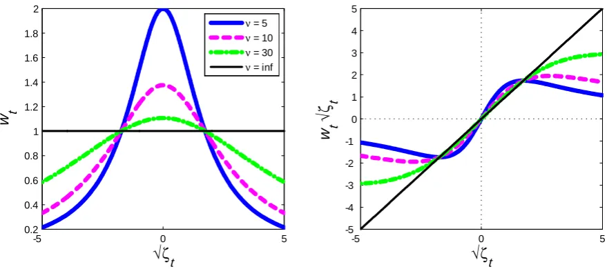
The crucial role played by the weights (19) is visualized by Figure 1. The left panel shows the magnitude of the weights wt as a function of the standardized prediction errors, while the

right one shows the weighted realizationswt p

twhich is known asin‡uence function in robust

statistics (see Maronna et al., 2006). Note that large innovations are categorized as being part of the tails of the distribution. As such they are downweighted and have a small e¤ect on the dynamic of the time-varying parameters.

[insert Figure 1]

Under Student-t distribution the score-driven algorithm leads to a robust …lter and gener-alizes the CGL algorithm (13).

Proposition 1 Under Student-t distribution the score-driven model leads to the following adaptive algorithm for the time-varying parameters

Rt = Rt 1+ h[ wt(xt _tjt2 ₁x0t Rt 1)]; (20)

t+1jt = tjt 1+ Rt1xt _tjt2 ₁[ wt(yt x0t tjt 1)]; 2

t+1jt =

2

tjt 1+ [(1 + 3 ) (wt"2t

2

tjt 1)];

with = [(1 2 ) (1 + 3 )=(1 + )], wt de…ned in (19) and = ( ; h; ; )0 is the

corre-sponding vector of static parameters. The magnitude of the weightswtdepends on how close the

actual observation is to the center of the distribution of "t: large deviations are downweighted

and a small value of wt is more likely with lower degree of freedom and lower dispersion of

the distribution. Therefore, the recursions above imply a double weighting scheme, i.e. the observations are weighted both across time and realizations, and the estimated time-varying parameters are robust to extreme events.

A simpli…ed version of model (15) helps clarify the impact of the double weighting. Assume that xt = 1 and wt is exogenously given. This speci…cation leads to an IMA(1,1) model with

time-varying moving average coe¢ cient(1 wt), and time-varying variance. The time-varying

mean can be expressed as follows

t+1jt= tjt 1+ wt(yt tjt 1) = 1 X

j=0

jeyt j =

1 (1 wt)Le

yt; (21)

with y_et j =wt jyt j. Speci…cally, equation (21) shows that the observations are: (i) weighted

across time with weights j = t Q

k=t j+1

(1 wk), 0 = 1 and = . This is equivalent

to a one-sided low-pass …lter with time-varying coe¢ cients, that is =[1 (1 wt)L], and

it implies a time-varying transfer function.17 Similarly, in order to estimate the variance 2t,

the squared prediction errors "2_{t j} are weighted by jwt, where the weights across time are

j = [1 (1 + 3 )]j, namely

2

t+1jt=

2

tjt 1+ (wt"2t

2

tjt 1) = 1 X

j=0

(1 )j_e"2_{t j} =

1 (1 )Le"

2

t; (22)

wheree"2_{t j} =wt j"2t jis the weighting across realizations, and =[1 (1 )L]is the standard

one-sided low-pass …lter, with = (1 + 3 ).

Remark 2 In practice the weights wt depend (non-linearly) on the current observations and

the past parameters’estimation through _t="2

t= 2tjt 1. Therefore, the score-driven model under

Student-t distribution solves a recursive stochastic Gauss-Newton algorithm for a non-quadratic loss function and it leads to a non-linear …lter. Therefore, it cannot be derived as a solution of quadratic loss function with re-weighted observations of the type discussed in Ljung and Soderstrom (1985, sec. 2.2).

5

Model restrictions

Applications of time-varying parameters models often require to impose restrictions on the parameters space. For instance, in the autoregressive model (1) it is customary to impose restrictions on the autoregressive coe¢ cients so that the implied roots are always within the unit circle, i.e. restrictions implying a locally stationary model. In the Bayesian framework constraints are usually imposed by rejection sampling (see e.g. Cogley and Sargent, 2005, and Koop and Potter, 2012). Thus, however, leads to heavy ine¢ ciencies.

General non-linear restrictions can be accommodated within the score-driven model. This requires to reparameterize the model with respect to a new vector of unconstrained parameters. De…ne the following transformation ft = g(eft); where ft is the original vector of parameters, eft is the new parametrization and g( ) is a continuous and twice di¤erentiable transformation

function, often known aslink function, which maps the new vector of unconstrained parameters into the space of constrained parameters. Following Creal et al (2012) and Harvey (2013), the score-driven model (3) can be expressed with respect to the new vector of parameters

eft+1jt=!e+Aeeftjt 1+Beest; (23)

where_est=Iet 1Oetis the scaled score computed with respect toeft=g 1(ft), where g 1( )is the

17_{The transfer function ca be expressed as follows G( ) = 1 + (1 wt)}2 _{2(1 wt) cos( )} 1=2_;

where 0 < < is the radian frequancy. See Dahlhaus (2012) for details on stationary processes with

inverse function of g( ). For a given continuous and di¤erentiable function g( ), the new score vector is then

e Ot=

@`t

@eftjt 1

=

"

@`t

@f0 tjt 1

@ftjt 1

@ef0 tjt 1

#0

= 0tOt;

where t = @ftjt 1=@ef_t0_{jt 1} is the Jacobian of g( ) and is deterministic given past information.

Therefore, the transformed scaling matrix is equal to _Iet= 0tIt t and the new scaled score is

then equal to

est= ( 0tIt t) 1 0tOt: (24)

The transformation function g(:) imposes (possibly) non-linear restrictions on the time-varying parameters. It is worth noticing that under Gaussian distribution, the non-linear …ltering problem can be solved by …rst order Taylor approximation. This argument is formalized in the Theorem below. Also in this case we can replace the scaling matrix_Ietwith its smoothed

version Rt= (1 h)Rt 1+ hIet.

Theorem 1 Consider the Gaussian model (14) and impose a non-linear transformation on the

coe¢ cients t=g( t). The model can be solved by the Extended KF of Anderson and Moore

(1979, sec. 8.2) and the implied algorithm is exactly equal to the score-driven …lter (23).

(Proof in the Appendix A.)

The constrained algorithm has been commonly implemented in the literature by means of the projection facility (see Ljung and Soderstrom, 1985, sec. 6.6, Timmermann, 1996, and Evans and Honkapohja, 1998). Speci…cally, they use a constant parameter weighting the driving process such that the incremental step is progressively shrunk until the restriction is satis…ed.18

The adaptive model (5), with (23)-(24), automatically achieves the same objective. In fact, the matrix tre-weights the Gauss-Newton search direction so that the restrictions are always

satis…ed. With respect to the standard projection facility, the re-weighting of our adaptive model varies at di¤erent points of the recursion and, most importantly, shrinks the search in the optimal way as opposed to the usual scalar shrinkage.

In the next sub-sections we illustrate how to implement speci…c restrictions which are commonly imposed to an autoregressive model with time-varying parameters.

5.1

Imposing stationarity

In this section we consider restrictions to the parameters space implying the model is locally stationary. This exploits the mapping between the coe¢ cients of an autoregressive model and its partial autocorrelations. Stationarity is then imposed by restricting the latter in the interval

( 1;1). To simplify the notation we start with model (1) without the intercept and then we consider the general model.

Proposition 2 For each point in time t, let t = ( 1;t; :::; p;t)0 denote the vector of

coef-…cients, t = ( 1;t; :::; p;t)0 the corresponding vector of partial autocorrelations and t =

( 1;t; :::; p;t)0 the vector of unrestricted coe¢ cients. A locally stationary model has t2Sp;

where Sp _{is the hyperplane with all roots, z}

t, inside the unit circle, i.e. t(zt) = 0; zt 2 Cp

and _jzj;tj < 1 for j = 1; :::; p. It is possible to show that t2Sp if and only if t 2 Rp and

j j;tj<1. Therefore, let t = ( t) de…ne the function mapping the coe¢ cients to the partial

autocorrelations and t = ( t) a function that restricts the partial autocorrelations to lie in

the region ( 1;1): The function t = ( t) is uniquely obtained by the last recursion of the

Durbin-Levinson algorithm

j;k t =

j;k 1

t k;t k j;kt 1 for j = 1; :::; k 1 and k = 2; :::; p; (25)

with 1t;1 = 1;t and tk;k = k;t. The function t= ( t) is any monotonic and di¤erentiable

function

j;t = ( j;t); such that j;t2( 1;1); j = 1; :::; p: (26)

The composite function g( ) = [ ( )] maps the restricted stationary coe¢ cients into the

un-restricted parameters, i.e. t=g( t) with t2( 1;1) and t2Sp.

(The Proof follows from Bandor¤-Nielsen and Schou, 1973, and Monahan, 1984).

The functions ( ) and ( ) are continuous and di¤erentiable and the Jacobian matrix is

t=

@g( t)

@ 0 t

= @ ( t)

@ 0 t

@ ( t)

@ 0 t

; (27)

where @ ( t)=@ 0t is diagonal matrix containing @ ( jt)=@ j;t with j = 1; :::; p, while the

analytic expression for @ ( t)=@ 0t = t is obtained in the theorem below.

Theorem 2 The Jacobian matrix t is obtained from the last iteration of the recursion

k;t = "

e_{k 1;t} bk 1;t 00_{k 1} 1

#

; (28)

e_{k 1;t} = Jk 1;t k 1;t; k = 2; :::; p;

with

bk 1;t = 2 6 6 6 6 6 6 6 4

k 1;k 1

t k 2;k 1

t

.. .

2;k 1

t

1;k 1

t 3 7 7 7 7 7 7 7 5

; Jk 1;t = 2 6 6 6 6 6 6 6 4

1 0 0 k;t

0 1 0 k;t 0

..

. . .. ...

0 k;t 0 1 0

k;t 0 0 1

3 7 7 7 7 7 7 7 5 : (29)

Note that if k is even the central element of Jk 1;t it is equal to (1 k;t). The recursion is

initialized with J1;t = (1 2;t) and 1;t = 1:

Given the elements of the scaled score vector s t=I t1O t (computed with respect to t),

the adaptive algorithm for the transformed coe¢ cients t is equal to

t+1jt= tjt 1+ ( 0tI t t) 1 0tO t; (30)

where t = g( t) and t = ( t) are computed as outlined in Proposition 2 and Theorem

2, respectively. When the time-varying intercept is included without any restrictions, i.e.

0;t = 0;t, the Jacobian matrix is modi…ed as follows

t=

@ _t @ 0 t

=

"

1 00 0 22;t

#

; (31)

where 22;t =@( 1;t; :::; p;t)0=@( 1;t; :::; p;t) as computed in Theorem 2.

5.2

Bounded trend

It is also often the case that in practice one wants to discipline the model so as to have a bounded conditional mean. Following Beveridge and Nelson (1981), a stochastic trend can be expressed in terms of long-horizon forecasts. For a driftless random variable, the Beveridge-Nelson trend is de…ned as the value to which the series is expected to converge once the transitory component dies out (see e.g. Benati, 2007 and Cogley et al, 2010), i.e.

limh!1Et(yt+h) = t. . Speci…cally, for a stationary time-varying autoregressive process,

local-to-date t approximation implies that the unconditional time-varying mean is equal to

t = 0;t=(1 Pp

j=1 j;t). In line with Cogley et al (2010), our speci…cation implies that the

detrended component, that is _eyt = (yt t), follows a locally stationary time-varying AR(p)

model, i.e. Pr_flimh!1Et(yet+h) = 0g= 1. Following Chan et al (2013), we want to restrict t 2[b; b].

Proposition 3 Let h( ) be any continuous and di¤erential function so that h( )₂[b; b]. The

restriction on t2[b; b] can be achieved with the following transformation

0;t =h( 0;t) 1 p X

j=1

j;t !

: (32)

The Jacobian matrix is then equal to

t=

@ _t @ 0 t

=

"

11;t 012;t 0 22;t

#

; (33)

where 22;t has been computed in Theorem 2, while 11;t and 012;t are

11;t =

@h( 0;t)

@ 0;t

1

p X

j=1

j;t !

where = (1;1; :::;1)0:

To summarize, for each time t, the recursion (30) is implemented as follows: …rst, the stationary AR coe¢ cients are computed following Proposition 2; second, the constrained in-tercept and the Jacobian matrix t are computed as described in Proposition 3 so that all

the necessary elements to update tjt 1 are then available. In this section we have shown how

to implement some popular restrictions in a score-driven setup and this leads to a non-linear …lter that can be implement in the Classical framework without incurring in the computational demanding simulation methods of Koop and Potter (2011) and Chan el al (2013).

6

Application to the in‡ation dynamics

We implement the adaptive model in the analysis of in‡ation dynamics. The change in the persistence of the in‡ation has been strongly supported by Cogley and Sargent (2001).19

Speci…cally, they …nd that the persistence of in‡ation in the United States rose in the early 1970s and remained high during this decade, before starting a gradual decline from the early 1980s until the present. Pivetta and Reis (2007) challenge these …ndings presenting evidence of a stable level of persistence throughout the sample. It is therefore interesting to examine those issues in the light of our model. Another issue that has received much attention in recent years is related to the presence of a time-varying level of trend-in‡ation (Cogley, 2002, and Stock and Watson, 2006). Speci…cally, trend-in‡ation is generally thought of as a measure of the public’s perception of the credibility of the central bank in‡ation targeting, (see Kozicki and Tinsley, 2001, and Faust and Wright, 2011). Furthermore, Clark and Doh (2011) and Chan et al. (2013) highlight how accurate estimates of trend-in‡ation can improve the in‡ation forecasts at a long-horizon.

Following Cogley and Sargent (2005) and Pivetta and Reis (2007), we estimate the following p-th order autoregressive representation for in‡ation:

t= 0;t+ p X

j=1

j;t t j+"t; "t 0; 2t ; t = 1; :::; n: (34)

This speci…cation is ‡exible enough to capture changes in the long-run trend as well as changes in the persistence of the deviation around the trend. In addition, it allows for variation in the volatility which has been proven to be particularly important to understand the dynamic of in‡ation (see e.g. Pivetta and Reis, 2007 and Clark and Doh, 2011). Those features are of foremost importance to understand the changes in in‡ation dynamic over the post-WWII sample. The literature has mainly focussed on the parameter-driven models, estimated by Bayesian methods.20

In the application we allow for various speci…cations of (34). Speci…cally, we …rst consider a model with time-varying trend-only (p = 0), then we allow for various speci…cations of

19_{Similar results are provided by Taylor (2000) and Brainard and Perry (2000).}

the autoregressive components (p = 1;2 and 4), and the time-varying mean 0;t is always

included. Chan et al. (2013) forcefully argue for imposing bounds on the long-run trend on the grounds that a level of the trend in‡ation that is too low (or too high) is inconsistent with the clear mandate of the central bank in‡ation stability. Therefore, for every speci…cation we also include a counterpart derived with a bound (between 0 and 5) on the long-run trend.21

Furthermore, we consider all speci…cations under Gaussian and Student-t innovations. Finally, partial autocorrelations are always bounded so as to impose local stationarity of the model and the variance is reparameterized so that it is always positive.

Stock and Watson (2007, SW hereafter) documents that when correctly speci…ed, a model featuring a time-varying trend-in‡ation is the best performing model for producing point fore-casts. Given the prominence of the SW benchmark, it is worth discussing how this model is related to the score-driven model (5) without the autoregressive terms. In SW the conditional mean and the measurement error are driven by two independent shocks with stochastic volatil-ity. The model then implies that in‡ation follows a reduced form IMA(1,1) with time-varying MA coe¢ cient and time-varying variance, where both parameters are driven by a convolu-tion of the two independent stochastic volatilities. The observaconvolu-tion-driven model also implies an IMA(1,1) which has time-varying variance but constant coe¢ cient under Gaussian innova-tions. Yet, as was pointed out in Section 4, when the Student-t distribution is considered the score-driven model produces an IMA(1,1) with both time-varying coe¢ cients and time-varying variance.

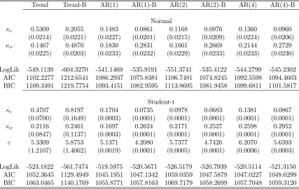
[Insert Table 1]

Table 1 reports the estimates for the various speci…cations for the annualized quarterly US-CPI in‡ation over the period 1955Q1–2012Q4. Besides the estimates of the parameters and their associated standard error, we also report the value of the log likelihood function and the Akaike (AIC) and Bayesian Information Criterion (BIC). The trend-only speci…cation with Gaussian innovations implies that the trend is estimated by the exponential smoothing as in Cogley (2002).22 _{This model features a high estimation of the smoothing parameter}

which implies a faster learning process. This is also true for all the speci…cations without autoregressive coe¢ cients. Adding the autoregressive components shows a substantially smaller estimate of the smoothing parameter as some of the persistence of in‡ation is now captured by the autoregressive terms. In contrast, the smoothing parameter associated to the variance equation is instead stable and typically higher than the one associated with the coe¢ cients, lending support to the idea that changes in the variance are particularly relevant in our sample (see also Pivetta and Reis, 2007). Noticeably, the speci…cations with Student-t distribution

21_{The bounds correspond to the upper and lower bounds in the posterior in Chen et al. (2013). They}

highlight that it is di¢ cult to identify exactly those bounds. They also show that, once the bounds are imposed to the autoregressive speci…cation, variations in the estimated long-run trend tends to be very limited. We also obtain a stable estimate for the long-run trend. This is typically not a¤ected by the choice of the upper and lower bound.

22_{Notice that with respect to the model in Cogley (2002) the speci…cation used as benchmark allows for}

always considerably outperform the ones with Gaussian innovations, as for the likelihood values and information criteria. In fact, the estimated low value of degrees of freedom depicts a remarkable di¤erence between the Gaussian and the Student-t speci…cation. The low value of suggests that there might be pronounced variations of in‡ation at the quarterly frequency. Those variations either arise from measurement issues or are related to the presence of rare events that structural macroeconomics should explicitly account for (as recently advocated by Curdia et al., 2013). Notice that = 5 is also consistent with the calibrated density forecast in Corradi and Swanson (2006). Furthermore, the AR(1) speci…cation without bounds on the long-run mean slightly outperforms all the others in terms of …tting.

6.1

Estimates of Trend In‡ation, Persistence, and Volatility

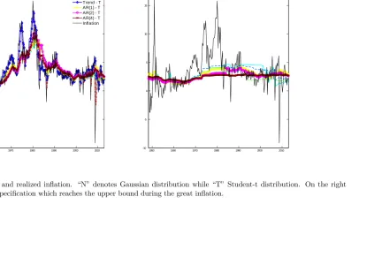
Figure 2 presents estimates of the long-run trend in in‡ation for the various speci…cations considered in this paper. The long-run trend, when is not bounded, tends to follow the underly-ing in‡ation, smoothunderly-ing away the transitory ‡uctuations. Some di¤erences can be appreciated when comparing the di¤erent speci…cations. The trend-only speci…cation follows in‡ation very closely trough the ups and downs. When we add autoregressive terms to the model, few di¤er-ences can be appreciated across various speci…cations. The inclusion of lags delivers a smoother long-run trend, suggesting that the high in‡ation in the early part of the sample and in the 70s is to be attributed to deviations from the trend. All speci…cations suggest that since the mid 90s, the long-run trend is stable between 2-3%, going slightly over 3% on the run up to the recent recession. Also, it is worth noticing that the speci…cation with Student-t are less a¤ected by the sharp transitory movements in in‡ation, in particular in the last part of the sample. Imposing the upper bound on the long-run mean implies a qualitatively similar pic-ture for the trend-in‡ation across the speci…cations.23 _{The trend is consistent with the idea}

of a central bank anchoring the expectations of trend-in‡ation to a fairly stable level over the sample. Trend-in‡ation rises above 3% in the early 70s and then decreases back to a slightly lower level only in the mid 90s. It is interesting to note that the pattern in the long-run trend is quite similar to the one found by Chan et al. (2012), although they use a di¤erent model speci…cation and estimation techniques.

[Insert Figure 2]

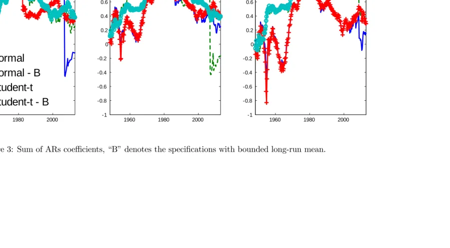
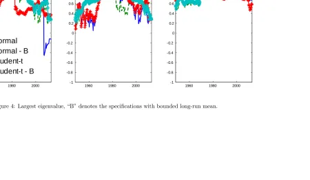
Moving to the analysis of the persistence in in‡ation, forp > 1 we follow Pivetta and Reis (2007) and compute both the sum of the AR coe¢ cients and the largest root as proxy of the overall persistence; those are shown in Figures 3 and 4. Similar to Cogley and Sargent (2001), most of our speci…cations tend to suggest that the persistence of in‡ation in the US rose in the early part of the sample to reach the pick during the great in‡ation of the 1970s, before starting a gradual decline from mid to late 1980s. Yet it is also interesting to note that allowing

23_{Figure 2 excludes the trend-bound speci…cation which is destined to reach the bounds during the great}

for a large number of lags tends to decrease the estimated persistence. This …nding reconciles the di¤erent results obtained by Pivetta and Reis (2007), who focus on time-varying AR model with three lags. It reports evidence of little variation in in‡ation persistence. Interestingly, the speci…cations with Student-t innovations are more robust to sharp variations which are due to the short lived spikes in the late part of the sample.

[Insert Figure 3]

[Insert Figure 4]

Figure 5 reports measures of the change in volatility. Some interesting issues emerge. All speci…cations show that the variance of in‡ation was substantially higher in the 50s, in the 70s and then again in the last decade. As in Chan et al. (2013), the trend-only speci…cations feature substantial di¤erences between bound versus unrestricted trend. Clearly, the bounded speci…cations overstate the level of volatility in the period when the bound is binding. Inter-estingly, if we compare Gaussian and Student-t distribution, they share similar low-frequency variation and the speci…cations with Student-t innovation display substantially more variation in the volatility. Consequently, with Student-t innovations the variance is less a¤ected by the outliers and it can better adjust to accommodate changes in the dispersion of the central part of the distribution. This latter result is particularly important in light of the considerable evidence in favor of the Student-t speci…cation reported in the previous sub-section. In fact, most of the macroeconomic literature, which has mainly focused on Gaussian distribution, has reported and emphasized the importance of the low frequency variation in the volatility. Fur-thermore, it is also worth mentioning that the measures based on the Student-t are also more robust to single outliers. Indeed, it is clear that under Gaussianity the volatility in the last part of the sample seems to be disproportionately a¤ected by very few observations.

[Insert Figure 5]

6.2

Forecasting Evaluation

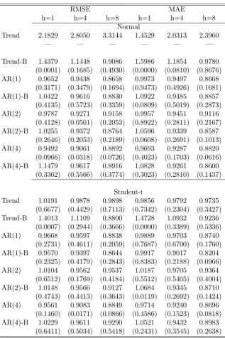
In this section we assess the forecasting performance of the various speci…cations. Speci…-cally, we evaluate the forecasts over the period 1973Q1–2012Q4, with the model re-estimated recursively over an expanding window. Consistent with a long-standing tradition in the learn-ing literature (referred to as anticipated-utility by Kreps, 1998), we update the coe¢ cients period by period and then treat the updated values as if they remained constant going forward in time. We …rst consider point forecast and use both root mean squared error (RMSE) and the absolute mean error (MAE). The speci…cation with trend-only and Gaussian innovation is taken as the benchmark model, as this is the closest speci…cation to the one of SW and it very close to the model of Cogley (2002).

substantial at longer forecast horizons, although in most of the cases the di¤erence in forecasting performance is not statistically signi…cant.24 A comparison between the Gaussian and Student-t models reveals liStudent-tStudent-tle di¤erences in Student-terms of poinStudent-t forecasStudent-t. Imposing bounds on Student-the long-run mean marginally enhances the performance of the various speci…cations, and in particular for the speci…cation with Student-t innovations.25

[Insert Table 2]

Table 3 reports the results from a density forecast exercise where we focus on the one-step-ahead forecast. A comparison of the average log score reveals that the models with Student-t innovations substantially improve in performance with respect to the ones with Gaussian inno-vations, regardless of the model.26 _{Furthermore, the table reports two tests for the calibration}

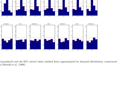
of the densities. One is the LR test on the inverse transformation of the PITs (Berkowitz, 2001) and the other is the nonparametric test of Rossi and Sekhposyan (2013, RS hereafter). The latter test remains valid also in the presence of parameter estimation error. The speci…cations with Gaussian innovations prove to be not well calibrated. In order to understand why this is the case Figure 6 plots the empirical distribution function (p.d.f.) of the PITs. In addition to the PITs, we also provide the 95% con…dence interval (broken lines) using a Normal approxi-mation to a binomial distribution as in Diebold et al. (1998). Figure 7 displays the cumulative distribution function (c.d.f.) of the PITs for each realization, under the null hypothesis the PITs should be uniformly distributed. Therefore the c.d.f. of the PITs should be the 45o _line.

The …gure also reports the critical values based on the RS test. If the c.d.f. of the PITs is outside the critical value lines, we conclude that the density forecast is not well calibrated.

[Insert Table 3]

From both …gures it is evident that the models with Gaussian innovations tend to produce densities where too many realizations fall in the middle of the forecast densities relative to what we would expect if the data were really Normally distributed.

[Insert Figure 6]

[Insert Figure 7]

In Table 4, for each pair of models, we report the p-values of the test of di¤erence in the average log predictive score using uniform weights, as outlined in Amisano and Giacomini

24_{Despite the expanding window, it is possible to apply the Giacomini and White (2006) test as the models}

implicitly discount the observations, so that the earlier observations tend to have limited or no relevance to the estimates in the late part of the sample that is used to forecast.

25_{The trend-only speci…cation with restricted long-run mean is always outperformed by the alternative ones,}

in particular for the short horizon. Anyway, the relative performance of this speci…cation is severely biased by the inclusions of the great in‡ation period (mid 70s-80s), as the model has an upper boundeat 5%.

26_{Clark and Ravazzolo (2012) document the gains of allowing for fatter tails. However, they found much}

(2007). The results con…rm that the substantial di¤erences between the Normal and Student-t are indeed signi…cant. At the same time, the p-values con…rm that some of the di¤erences across the various speci…cations with Student-t innovations are signi…cative, but none of the various speci…cations clearly outperforms the others.

[Insert Table 4]

The adaptive model developed in this paper delivers a model-consistent algorithm in pres-ence of heavy tails distribution. Appendix B explores the importance of using a law of motion for the parameters consistent with the score-driven model as opposed to some ad-hoc spec-i…cations. We show that the score-driven speci…cation outperforms the alternative ones: in particular, both the low degree of freedom and the score-driven law of motion, are important to achieve a well calibrated density forecasts.

Concluding, the empirical exercise shows that the model with Student-t distribution pro-duces time variation in the parameters which are robust to the presence of heavy tails. Fur-thermore, the volatility is less a¤ected by the behavior in the tail of the distribution so that it can better re‡ect the changes in the spread of the central part of the density. These aspects of the model are key in order to retrieve well calibrated density forecast for in‡ation over the sample analyzed.

7

Conclusion

In this paper we derive an adaptive algorithm for time-varying autoregressive models, both under Gaussianity and with heavy tails using a Student-t distribution. Following Creal et al. (2012) and Harvey (2013), the score of the conditional distribution is the driving process for the evolution of the parameters. This approach extends the least squares algorithms popularized by Ljung and Soderstrom (1985) - which are the building block of the learning expectation literature - to non-quadratic criterion functions. Furthermore, the algorithm is extended to incorporate restrictions which are popular in the empirical literature. Speci…cally, the model is allowed to have a bounded long-run mean and the coe¢ cients are restricted so that the model is locally stationary. Moreover, the adaptive algorithm is extended to an environment with changes in volatility and non-Gaussian distribution. The latter extension robusti…es the standard adaptive algorithms to the presence of tail events. With regards to the parameter-driven models, the route taken in this paper does not require the use of simulation techniques and thus has a clear computational advantage especially when restrictions on the parameters are imposed.

in‡ation, especially in the last decade. Furthermore, the use of heavy-tails highlights the presence of high-frequency variations in the volatility on top of the well documented low-frequency variations.

References

Abraham, B. and J. Ledolter (1983). Statistical Model for forecasting. Wiley.

Anderson, B.D.O. and J.B. Moore (1979). Optimal Filtering. Prentice Hall Englewood.

Bandor¤-Nielsen, O. and G. Shou (1973). On the Parametrization of Autoregressive Models by Partial Autocorrelations. Journal of Multivariate Analysis, 3, 408-419.

Benati, L. (2007). Drift and breaks in labor productivity,Journal of Economic Dynamics and Control, 31(8), 2847-2877.

Benati L. and H. Mumtaz (2007) The U.S. evolving macroeconomic dynamics: a structural investigation. ECB- Working Paper Series 0746.

Benveniste, A., Metivier, M. and P. Priouret (1990). Adaptive algorithms and stochastic

approximations. Springer-Verlag.

Berkowitz, J. (2001). Testing Density Forecasts with Applications to Risk Management.

Journal of Business and Economic Statistics, 19, 465-474.

Beveridge, S. and C.R. Nelson (1981). A new approach to decomposition of economic time se-ries into permanent and transitory components with particular attention to measurement of the business cycle. Journal of Monetary Economics, 7, 151-174.

Blasques F., Koopman S.J. and A. Lucas (2014). Time-Varying Temporal Dependence in Au-toregressive Models: An Observation Driven Approach. Tinbergen Institute Discussion Papers.

Brainard, W. and G. Perry (2000). Making policy in a changing world. In: Perry, G., Tobin, J. (Eds.), Economic Events, Ideas, and Policies: and Policies: The 1960s and After. Brookings Institution Press, Washington.

Bollerslev, T. (1987). A Conditionally Heteroskedastic Time Series Model for Speculative Prices and Rates of Return. Review of Economics and Statistics, 69, 542-547.

Branch, W.A. and G.W. Evans (2006). Simple Recursive Forecasting model.Economic Letter, 91, 158-166.

Brown, R.G. (1963). Smoothing, forecasting and prediction. Prentice Hall.

Canova, F. and L. Gambetti (2009). Structural changes in the US economy: Is there a role for monetary policy? Journal of Economic Dynamics and Control, Elsevier, 33(2), 477-490.

Casals, J., Jerez, M. and S. Sotoca (2002). An Exact Multivariate Model-Based Structural Decomposition. Journal of the American Statistical Association, 97, 553-564.

Chan, J.C.C., Koop, G. and S.M. Potter (2013). A New Model of Trend In‡ation. Journal

of Business and Economic Statistics, 31(1), 94-106.

Chiu, Ching-Wai, H. Mumtaz and G. Pinter (2014). Fat-tails in VAR Models. Working Papers 714, Queen Mary, University of London, School of Economics and Finance.

Clark, T.E. and XX. Doh (2011). A Bayesian Evaluation of Alternative Models of Trend In‡ation. Kansas City FED WP2011-16.

Clark, T.E. and F. Ravazzolo (2012). The macroeconomic forecasting performance of au-toregressive models with alternative speci…cations of time-varying volatility. WP-1218, Cleveland FED.

Cogley, T. (2002). A Simple Adaptive Measure of Core In‡ation. Journal of Money, Credit and Banking, 34(1), 94-113.

Cogley, T. and T.J. Sargent (2001). Evolving Post World War II U.S. In In‡ation Dynamics.

NBER Macroeconomics Annual,16.

Cogley, T. and T.J. Sargent (2005). Drifts and Volatilities: Monetary Policies and Outcomes in the Post WWII US. Review of Economic Dynamics, 8(2), 262-302.

Cogley, T., Primiceri, G. and T.J. Sargent (2010). In‡ation-Gap persistence in the US.

American Economic Journal: Macroeconomics, 2(1), 43-69.

Cooley, T. F. and E.C. Prescott (1973). An Adaptive Regression Model. International

Eco-nomic Review, 14(2), 364-71.

Cooley, T. F. and E.C. Prescott (1976). Estimation in the Presence of Stochastic Parameter Variation. Econometrica, 44(1), 167-84.

Corradi, V. and N.R. Swanson (2006). Predictive Density and Conditional Con…dence Interval Accuracy Tests. Journal of Econometrics, 135, (1-2),187-228.

Creal, D., Kopman, S.J. and A. Lucas (2012). Generalised Autoregressive Score Models with Applications. Journal of Applied Econometrics, 28, 777-795.

Cox, D.R. (1981). Statistical analysis of time series: some recent developments. Scandinavian Journal of Statistics, 8(2), 93-115.

Cúrdia, V., Del Negro, M. and D.L. Greenwald (2013). Rare shocks, Great Recessions. San

Francisco FED, WP 2013-01.

Dahlhaus, R. (2012). Locally stationary processes. Handbook of Statistics, Time Series Analy-sis: Methods and Applications. Ed. T.S. Rao, S.S. Rao and C.R. Rao, (30), 351-413.

Diebold, F.X , Gunther, T.A. and S.A. Tay (1998). Evaluating Density Forecasts with Appli-cations to Financial Risk Management. International Economic Review, 39(4), 863-83.

Durbin, J. and S.J. Koopman (2001). Time Series Analysis by State Space Methods. Oxford University Press.

Evans, G.W. and S. Honkapohja (1998). Convergence of learning algorithms without a pro-jection facility. Journal of Mathematical Economics, 30, 59-86.

Evans, G.W. and S. Honkapohja (2001). Learning and Expectations in Macroeconomics.

Princeton University Press.

Evans, G.W., Honkapohja, S. and N. Williams (2010). Generalized Stochastic Gradient

Learn-ing. International Economic Review, 51, 237-262.

Fagin, S.L. (1964). Recursive linear regression theory, optimal …lter theory, and error analysis of optimal systems. IEEE International Conv. Record, 12, 216-240.

Faust, J. and J.H Wright (2013). Forecasting In‡ation. Handbook of Economic Forecasting,

forthcoming, Vol 2A, Elliott G. and A. Timmermann Eds. North Holland.

Fiorentini, G., Calzolari, G. and L. Panattoni (1996). Analytical Derivatives and the Com-putation of GARCH Models. Journal of Applied Econometrics, 11, 399-417.

Fiorentini, G., Sentana, E. and G. Calzolari (2003). Maximum Likelihood Estimation and Inference in Multivariate Conditionally Heteroskedastic Dynamic Regression Models with Student t Innovations. Journal of Business and Economic Statistics, 21(4), 532-46.

Giraitis, L., Kapetanios, G. and T. Yates (2011). Inference on stochastic timevarying coe¢ -cient models. Queen Mary Univeristy of London, WP540.

Giacomini, R. and H. White (2006). Tests of Conditional Predictive Ability. Econometrica, 74(6), 1545-1578.

Hamilton, J.D. (1986). A standard error for the estimated state vector of a state-space model.

Journal of Econometrics, 33(3), 387-397.

Harvey, A.C. (1989). Forecasting, structural time series models and Kalman …lter. Cambridge University Press.

Harvey, A.C. (2013). Dynamic Models for Volatility and Heavy Tails. With Applications to

Financial and Economic Time Series. Cambridge University Press.

Hyndman, R.J., Koehler, A.B., Ord, J.K. and R.D. Snyder (2008). Forecasting with

Expo-nential Smoothing: The State Space Approach. Springer.

Jazwinski, A.H. (1970). Stochastic Processes and Filtering Theory. Academic Press, San Diego.

Justiniano, A. and G. Primiceri (2008). The Time-Varying Volatility of Macroeconomic Fluc-tuations. American Economic Review, 98(3), 604-641.

Kim, C-J. and C. Nelson (1999). State-Space Models with Regime Switching: Classical and

Gibbs-Sampling Approaches with Applications. MIT Press.

Koop, G. and D. Korobilis (2009). Bayesian Multivariate Time Series Methods for Empirical Macroeconomics. Foundations and Trends in Econometrics, 3 (4), 267–358.

Koop, G. and D. Korobilis (2012). Large Time Varying Parameter VARs. Journal of Econo-metrics, forthcoming.

Koop, G. and S.M. Potter (2011). Time varying VARs with inequality restrictions. Journal of Economic Dynamics and Control, 35(7), 1126-1138.

Kozicki, S. and P.A. Tinsley (2001). Term structure views of monetary policy under alterna-tive models of agent expectations. Journal of Economic Dynamics and Control, 25(1-2), 149-184.

Kreps, D. (1998). Anticipated Utility and Dynamic Choice. 1997 Schwartz Lecture, in Fron-tiers of Research in Economic Theory, Edited by D.P. Jacobs, E. Kalai, and M. Kamien.

Cambridge University Press.

Li, H. (2008). Estimation and testing of Euler equation models with time-varying reduced-form coe¢ cients. Journal of Econometrics, 142, 425-448.

Ljung, L. (1992). Stochastic approximation and optimization of random system. Georg P‡ug, Harro Walk - Basel [etc.]. Birkhauser.

Ljung, L. (1999) System Identi…cation. Theory for the User. Prentice Hall. 2nd Eds.

Ljung, L. and T. Soderstrom (1985). Theory and Practice of Recursive Identi…cation. MIT Press.

Lucas, R. Jr (1976). Econometric policy evaluation: A critique. Carnegie-Rochester

Confer-ence Series on Public Policy, 1(1),19-46.

Marcet, A and T. Sargent (1989). Convergence of least squares learning mechanisms in self-referential linear stochastic models. Journal of Economic Theory, 48(2), 337-368.

Monahan, J.F. (1984). A note on enforcing stationarity in autoregressive-moving average models. Biometrika, 71(2), 403-404.

Montgomery, D.C. and L.A. Johnson (1976). Forecasting and time series analysis. Mc Graw-Hill.

Pesaran, M.H. and A. Timmermann (2007). Selection of estimation window in the presence of breaks. Journal of Econometrics, Elsevier, 137(1), 134-161.

Pesaran, M.H. and A. Pick (2011). Forecast Combination across Estimation Windows. Jour-nal of Business Economics and Statistics, 29, 307-318.

Pesaran, M.H., Pick, A. and M. Pranovich (2013). Optimal Forecasts in the Presence of Structural Breaks. Journal of Econometrics (forthcoming).

Pivetta, F. and R. Reis (2007). The persistence of in‡ation in the United States. Journal of Economic Dynamics and Control, 31(4), 1326-1358.

Primiceri, G. (2005). Time Varying Structural Vector Autoregressions and Monetary Policy.

The Review of Economic Studies, 72, 821-852.

Rossi, B. and T. Sekhposyan (2013). Conditional Predictive Density Evaluation in the Pres-ence of Instabilities. WP688, Barcelona Graduate School of Economics.

Sargent, T.J. (1999). The Conquest of American In‡ation. Princeton University Press.

Sargent, T.J., and N. William (2005). Impacts of priors on convergence and escapes from Nash in‡ation. Review of Economic Dynamics, 8, 360-391.

Sargent, T.J., William, N. and T. Zha (2006). Shocks and Government Beliefs: The Rise and Fall of American In‡ation, American Economic Review, 96(4), 1193-1224.

Slobodyan S. and R. Wouters (2012). Learning in an estimated medium-scale DSGE model.

Journal of Economic Dynamics and Control, 36(1), 26-46.

Stock, J. and M. Watson (1996). Evidence on Structural Instability in Macroeconomic Time Series Relations. Journal of Business and Economic Statistics, 14(1), 14-30.

Stock, J. and M. Watson (2007). Why has U.S. in‡ation become harder to forecast? Journal of Money, Credit and Banking 39(F), 3-33.

Taylor, J. (2000). Low in‡ation, pass-through, and the pricing power of …rms. European Economic Review 44 (7), 1389–1408.

Trend Trend-B AR(1) AR(1)-B AR(2) AR(2)-B AR(4) AR(4)-B Normal

c 0.5309 0.2055 0.1483 0.0861 0.1168 0.0976 0.1360 0.0960

(0.0214) (0.0221) (0.0227) (0.0201) (0.0215) (0.0209) (0.0224) (0.0206)

0.1467 0.4870 0.1830 0.2831 0.1661 0.2669 0.2144 0.2729

(0.0225) (0.0203) (0.0233) (0.0232) (0.0229) (0.0233) (0.0233) (0.0230)

LogLik -549.1139 -604.3270 -541.1469 -535.9191 -551.3741 -535.4122 -544.2799 -545.2302

AIC 1102.2277 1212.6541 1086.2937 1075.8381 1106.7481 1074.8245 1092.5598 1094.4603

BIC 1109.3491 1219.7754 1093.4151 1082.9595 1113.8695 1081.9458 1099.6811 1101.5817

Student-t

c 0.4707 0.8197 0.1704 0.0735 0.0978 0.0683 0.1381 0.0867

(0.0700) (0.1649) (0.0003) (0.0001) (0.0001) (0.0001) (0.0001) (0.0001)

0.2116 0.2461 0.1697 0.2624 0.2171 0.2527 0.2598 0.2952

(0.0847) (0.1137) (0.0003) (0.0001) (0.0001) (0.0001) (0.0001) (0.0001)

5.3309 5.8753 5.1371 4.2080 5.7377 4.7426 6.2070 5.6393

(1.2107) (1.4062) (0.0019) (0.0001) (0.0005) (0.0001) (0.0006) (0.0003)

LogLik -523.1822 -561.7474 -519.5975 -520.5671 -526.5179 -520.7939 -520.5114 -521.3150

AIC 1052.3645 1129.4949 1045.1951 1047.1342 1059.0359 1047.5879 1047.0227 1048.6299

BIC 1063.0465 1140.1769 1055.8771 1057.8163 1069.7179 1058.2699 1057.7048 1059.3120

Table 1: Estimation of the annualized quarterly US-CPI in‡ation, t = 400 logpt, sample

1955Q1-2012Q4. “Trend” denotes the speci…cation without ARs coe¢ cients (p = 0), “B” denotes the speci…cations with restricted long-run mean, and c, and are the static

RMSE MAE

h=1 h=4 h=8 h=1 h=4 h=8

Normal

Trend 2.1829 2.8050 3.3144 1.4529 2.0313 2.3960

— — — — — —

Trend-B 1.4379 1.1448 0.9086 1.5986 1.1854 0.9780

(0.0001) (0.1685) (0.4930) (0.0000) (0.0810) (0.8676)

AR(1) 0.9652 0.9438 0.8658 0.9973 0.9497 0.8668

(0.3171) (0.3479) (0.1694) (0.9473) (0.4926) (0.1681)

AR(1)-B 1.0422 0.9616 0.8830 1.0922 0.9485 0.8857

(0.4135) (0.5723) (0.3359) (0.0809) (0.5019) (0.2873)

AR(2) 0.9787 0.9271 0.9158 0.9957 0.9451 0.9116

(0.4128) (0.0501) (0.2053) (0.8922) (0.2811) (0.2167)

AR(2)-B 1.0255 0.9372 0.8764 1.0596 0.9339 0.8587

(0.2646) (0.2053) (0.2189) (0.0608) (0.2691) (0.1013)

AR(4) 0.9492 0.9061 0.8892 0.9693 0.9287 0.8820

(0.0966) (0.0318) (0.0726) (0.4023) (0.1703) (0.0616)

AR(4)-B 1.1479 0.9617 0.8916 1.0828 0.9261 0.8600

(0.3362) (0.5566) (0.3774) (0.3023) (0.2810) (0.1437)

Student-t

Trend 1.0191 0.9878 0.9898 0.9856 0.9792 0.9735

(0.6677) (0.4429) (0.7113) (0.7342) (0.2304) (0.3427)

Trend-B 1.4013 1.1109 0.8800 1.4728 1.0932 0.9236

(0.0007) (0.2944) (0.3666) (0.0000) (0.3389) (0.5336)

AR(1) 0.9668 0.9597 0.8838 0.9889 0.9703 0.8740

(0.2731) (0.4611) (0.2059) (0.7687) (0.6700) (0.1760)

AR(1)-B 0.9570 0.9397 0.8644 0.9917 0.9017 0.8204

(0.2325) (0.4179) (0.2843) (0.8383) (0.2188) (0.0966)

AR(2) 1.0104 0.9562 0.9537 1.0187 0.9705 0.9364

(0.6512) (0.1769) (0.4184) (0.5512) (0.5405) (0.4004)

AR(2)-B 1.0148 0.9566 0.9127 1.0684 0.9345 0.8710

(0.4743) (0.4413) (0.3643) (0.0119) (0.2692) (0.1424)

AR(4) 0.9561 0.9083 0.8849 0.9714 0.9240 0.8696

(0.1460) (0.0171) (0.0866) (0.4586) (0.1523) (0.0818)

AR(4)-B 1.0229 0.9611 0.9290 1.0521 0.9432 0.8983

(0.6411) (0.5034) (0.5418) (0.2431) (0.3545) (0.2638)

ALogS LR RS ALogS LR RS

Normal Student-t

Trend -2.5591 0.1445 4.4223 -1.5897 0.7000 0.7023

Trend-B -3.1073 0.0581 7.8323 -1.5688 0.0048 0.2723

AR(1) -2.4857 0.0041 3.7823 -1.6325 0.9976 0.1322

AR(1)-B -2.4543 0.0046 3.1923 -1.6766 0.9946 0.0423

AR(2) -2.5357 0.0058 4.6922 -1.6249 0.5005 0.5522

AR(2)-B -2.6275 0.4572 3.7210 -1.6671 0.7590 0.3610

AR(4) -2.4663 0.1455 3.4810 -1.5976 0.7914 0.2560

AR(4)-B -2.6022 0.9784 4.0960 -1.6272 0.7549 1.3323