Bayesian inference for indirectly observed stochastic processes, applications to epidemic modelling

Indirectly Observed Stochastic Processes,

Applications to Epidemic Modelling

J

OSEPH

DUREAU

S

K

K

W

B

Thesis submitted to the Department of Statistics

of the London School of Economics and Political Sciences

Declaration

The times after Copernicus were times in which there were great debates about whether the planets in fact went around the sun along with the earth, or whether the earth was at the centre of the universe and so on. Then a man namedTycho Braheevolved a way of answering the question. He thought that it might perhaps be a good idea to look very very carefully and to record exactly where the planets appear in the sky, and then the alternative theories might be distinguished from one another.

I would first like to thank Kostas Kalogeropoulos for his patience, enthusiasm and constant implication in supervising my first steps as a statistician; it has truly been a pleasure. I also thank John Edmunds and Arnaud Doucet, who have taken the time to read, examine and discuss this manuscript.

I am grateful to Bernard Cazelles for introducing me to the world of epidemiology, inspiring this project and supporting me during the third year of the PhD. I also wish to thank all the researchers with whom I have collaborated on the questions explored in this thesis: Marc Baguelin, Marie-Claude Boily, Peter Vickerman, Michael Pickles and Alex Beskos. This work has also been possible thanks to enriching discussions with Sebastien Ballesteros, Anton Camacho, and Nikos Demiris, who have nourished my reflexion and motivation.

I have enjoyed being part of the Statistics department of the London School of Eco-nomics, and particularly thank Irini Moustaki, Chris Skinner, Whicher Bergsma, Pauline Barrieu and Ian Marshall for financial and human support.

I am deeply endebted to Cyrille Henry-Bonniot, Jérémie Triolet and Marine Ricci for making my visits to London restful, joyful and stimulating. Many thanks as well to all the other London folks: Hugo Maisonhaute, Flavia Giammarino, Yehuda Dayan, Mai Hafez, Raphaelle Metras and Guillaume Fournié.

I wish to express my gratitude to my friends and family for having born with me during these years of doubt and obsession. At last, this would not have been possible without the permanent support of Lucile. Thank you.

Stochastic processes are mathematical objects that offer a probabilistic representation of how some quantities evolve in time. In this thesis we focus on estimating the trajectory and parameters of dynamical systems in cases where only indirect observations of the driving stochastic process are available. We have first explored means to use weekly recorded numbers of cases of Influenza to capture how the frequency and nature of contacts made with infected individuals evolved in time. The latter was modelled with diffusions and can be used to quantify the impact of varying drivers of epidemics as holidays, climate, or prevention interventions. Following this idea, we have estimated how the frequency of condom use has evolved during the intervention of the Gates Foundation against HIV in India. In this setting, the available estimates of the proportion of individuals infected with HIV were not only indirect but also very scarce observations, leading to specific difficul-ties. At last, we developed a methodology for fractional Brownian motions (fBM), here a fractional stochastic volatility model, indirectly observed through market prices.

The intractability of the likelihood function, requiring augmentation of the parameter space with the diffusion path, is ubiquitous in this thesis. We aimed for inference methods robust to refinements in time discretisations, made necessary to enforce accuracy of Euler schemes. The particle Marginal Metropolis Hastings (PMMH) algorithm exhibits thismesh freeproperty. We propose the use of fast approximate filters as a pre-exploration tool to estimate the shape of the target density, for a quicker and more robust adaptation phase of the asymptotically exact algorithm. The fBM problem could not be treated with the PMMH, which required an alternative methodology based on reparameterisation and ad-vanced Hamiltonian Monte Carlo techniques on the diffusion pathspace, that would also be applicable in the Markovian setting.

Table of Contents 11

List of tables 14

List of Figures 16

1 Introduction 23

1.1 Modelling the spread of infectious diseases . . . 23

1.1.1 Diverse situations and challenges . . . 24

1.1.2 The dynamics of epidemics . . . 25

1.1.3 Inference, a hypothetico-deductive approach . . . 27

1.1.4 Applications in public health . . . 28

1.1.5 Mathematical formulation of epidemic dynamics . . . 29

1.2 Bayesian inference . . . 38

1.2.1 General framework for indirectly observed stochastic processes 38 1.2.2 Simulation schemes . . . 41

1.2.3 The Monte Carlo Markov Chain machinery . . . 44

1.2.4 Exploring sequentially structured distributions: particle filtering 46 1.2.5 Full inference for stochastic processes . . . 48

1.3 Plan and contributions of the thesis . . . 50

1.3.1 Capturing the time-varying drivers of an epidemic using stochas-tic dynamical systems . . . 50

1.3.2 Estimating changes in condom use from limited HIV preva-lence data . . . 50

1.3.3 Bayesian inference with the advanced HMC algorithm . . . 51

2 Capturing the time-varying drivers of an epidemic 53

2.1 Introduction . . . 53

2.2 Modelling framework . . . 54

2.2.1 Epidemic models with time-varying coefficients . . . 54

2.2.2 Diffusion driven epidemic models . . . 56

2.3 Data augmentation via MCMC . . . 57

2.3.1 Model and data augmentation setup . . . 57

2.3.2 Data augmentation via Gibbs schemes . . . 58

2.3.3 Adaptive particle Markov Chain Monte Carlo algorithms . . . . 59

2.4 Simulation experiments . . . 61

2.5 The 2009 A/H1N1 pandemic . . . 65

2.5.1 Data, model and estimates . . . 65

2.5.2 Application in real time. Was the first wave waning due to de-pletion of susceptibles? . . . 67

2.5.3 A multiple age group diffusion driven SEIR model . . . 70

2.6 Towards an extended framework . . . 74

2.6.1 Generalisation of the use of time-varying parameters . . . 75

2.6.2 Diffusion approximation of the demographic stochasticity . . . 76

2.6.3 Diffusion approximation of the environmental stochasticity . . 79

2.6.4 Gaussian SDE approximation in the general case . . . 80

2.7 Discussion . . . 80

3 Estimating changes in condom use from limited data 83 3.1 Introduction . . . 83

3.2 Models and methods . . . 85

3.2.1 HIV transmission model for female sex workers . . . 85

3.2.2 Trajectory priors for condom use . . . 89

3.2.3 Priors . . . 92

3.2.4 Computational schemes for implementation . . . 92

3.3 Evaluation methodology based on ensemble simulations . . . 94

3.3.1 Parameter of interest . . . 95

3.3.2 Measures of performance . . . 95

3.3.3 Simulation procedure . . . 96

3.4 Results . . . 97

3.4.1 Comparison of the CU trajectory models from ensemble simu-lations . . . 97

3.5 Generalisation, and integration of survey-based estimates . . . 101

3.5.1 Impact estimators derived from limited prevalence data . . . . 101

3.5.2 Contrast of model outputs with survey-based condom use es-timates . . . 104

3.5.3 Bayesian synthesis and final estimates . . . 105

3.6 Discussion . . . 107

4 The advanced Hybrid Monte Carlo algorithm 109 4.1 Introduction . . . 109

4.2 An efficient MCMC sampler . . . 110

4.2.1 A priori decouplingx0:nandθ . . . 111

4.2.2 Classic version of the Hybrid Monte Carlo algorithm . . . 111

4.2.3 Advanced Hybrid Monte Carlo algorithm . . . 113

4.2.4 Scaling mass matrix . . . 114

4.3 Application: fractional stochastic volatility model . . . 115

4.3.1 A long-memory stochastic volatility model . . . 115

4.3.2 O(NlogN)implementation of the advanced HMC on a frac-tional stochastic volatility model . . . 118

4.3.3 Simulation and Results . . . 121

4.4 Discussion . . . 128

5 Future Research 131 5.1 Bayesian inference for sparse high-dimensional systems . . . 131

5.2 Sequential advanced Hybrid Monte Carlo Algorithm . . . 133

5.3 Epidemic dynamics and climate: a mechanistic exploration . . . 134 A Supplementary material for Chapter 2 137

B Supplementary material for Chapter 4 141

2.1 Mean, median and95%confidence intervals forτ andσestimates in four

experiments. . . 62 2.2 Relative efficiency of the different versions and initialisations of the

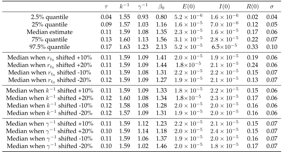
adap-tive PMCMC algorithm, via the minimum ESS (%) after adaptation. . . 65 2.3 Original estimates compared to the ones resulting from respectively tilting

the priors onrt0,γ

−1_ork−1_{by +10, +20, -10 or -20% . . . . 68}

2.4 Mean, median and95%confidence intervals for the parameters of the

struc-tured model applied to the A/H1N1 pandemic data . . . 74 3.1 Table of priors for the different components of{θi.c., θtr., θCU} . . . 93

3.2 Frequentist properties of the different estimators of the amplitude of the

shift in condom use during the intervention, estimated from 100 simulations 100 3.3 General distinctive power (AUC) of the median estimator of the shift, and

specific sensitivity and specificity when answering: is the shift in CU dur-ing the intervention stronger than 0.2? than 0.4? These quantities were

estimated over 100 simulations. . . 100 3.4 Estimates of the change in CU in Mysore between 2003 and 2009. . . 101 3.5 Prevalence estimates in each region with corresponding years. . . 103 3.6 ∆CU indirectly estimated from prevalence data in each region, with

asso-ciated credible intervals . . . 104 3.7 Survey-based estimate at first IBBA and estimated progression untill last

IBBA. Model-based estimates of the corresponding quantities indirectly

es-timated from prevalence data. . . 105 3.8 ∆CU estimates in each region with associated credible intervals resulting

from the Bayesian synthesis of prevalence data and biased survey estimates 107

4.1 Relative efficiency of the different implementations of the advanced HMC algorithm on Dataset 1 (H = 0.5), via the minimum ESS (%) and CPU times

(seconds). . . 123 4.2 Relative efficiency of the different implementations of the advanced HMC

algorithm on Dataset 2 (H = 0.85), via the minimum ESS (%) and CPU

times (seconds). . . 123 4.3 Relative efficiency, via the minimum ESS (%) and CPU times (seconds). In

this case, the mass (M) and sampling covariance (Σq) matrices are set to the

Identity matrix. . . 126 4.4 Relative efficiency, via the minimum ESS (%) and CPU times (seconds). In

this case, the mass (M) and sampling covariance (Σq) matrices are set to the

posterior density Covariance matrix. . . 127 A.1 Mean Squarred Error and Bias ofβtestimates provided by the EKF, particle

1.1 Representation of the different epidemic models introduced in the thesis . . 36

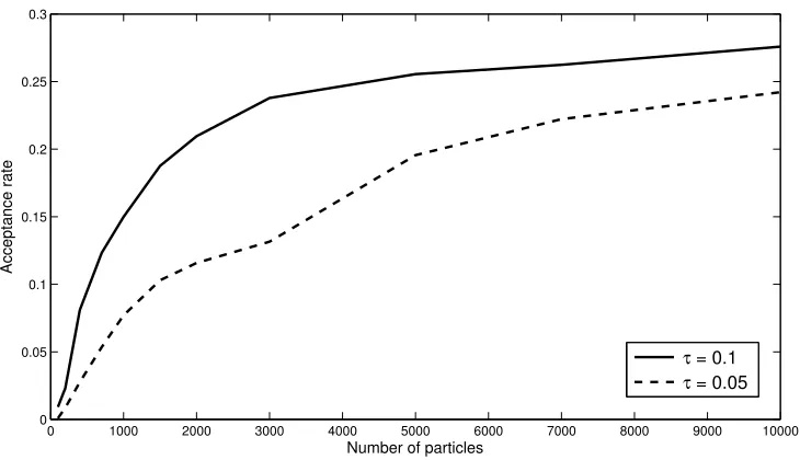
2.1 Acceptance rate as a function ofJ . . . 62

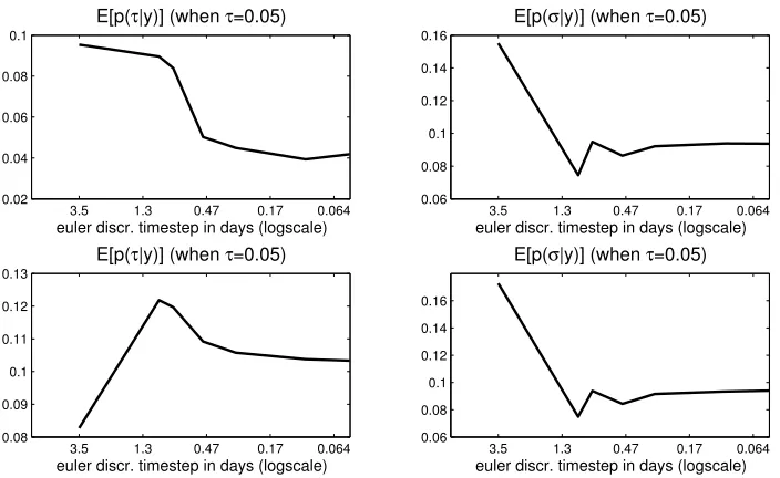
2.2 Convergence of the posterior density as the Euler discretization time-stepδ decreases . . . 63

2.3 Illustration of how the underlying dynamic of the effective contact rate can be estimated from weekly recorded cases. . . 64

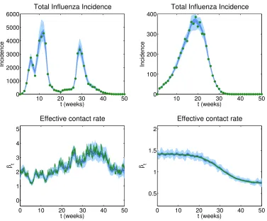
2.4 Weekly incidence data from the A/H1N1 2009 influenza pandemic and cor-responding offline estimates of the effective contact rate. . . 66

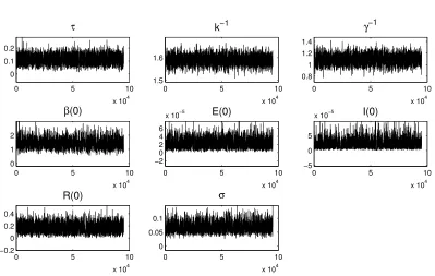
2.5 MCMC traceplots for each component ofθ . . . 67

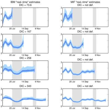
2.6 What could have been inferred by carefully following the epidemic in real time? . . . 69

2.7 Modeling choices and implications, aiming for robustness . . . 70

2.8 The implication of different scenarios for the real value of underreporting on the decrease of the effective contact rate between July13thand August1st 71 2.9 Offline estimates of the effective contact rate among children and adults during the A/H1N1 2009 influenza pandemic using a 2-classes age-structured model and age-specific incidence data . . . 73

2.10 Representation of the different models introduced in the thesis . . . 77

2.11 Unidentifiable parameters . . . 81

3.1 Flow-diagram of the model for high-risk FSWs . . . 87

3.2 Simulation procedure, repeated 100 times for each trajectory prior . . . 97

3.3 ROC curve when testing for∆CU >0.2and∆CU >0.4, under Brownian motion trajectory prior . . . 98

3.4 Bias of each model as a function of the true amplitude of the shift in condom

use, estimated from 100 simulations. . . 99 3.5 CU trajectory estimates obtained for Mysore district . . . 102 3.6 Condom use estimated trajectories resulting from the Bayesian synthesis

of prevalence estimates, the HIV transmission model and cross-sectional

behavioural surveys including survey-based condom use estimates . . . 106 4.1 Realisations of the fractional brownian motion . . . 118 4.2 Simulated paths of fractional stochastic volatility . . . 121 4.3 Posterior marginal densities for the different parameters of the model with

Dataset 1 (H=0.7) . . . 124 4.4 Posterior marginal densities for the different parameters of the model with

Dataset 2 (H=0.85). . . 124 4.5 Simulated paths of fractional stochastic volatility with respective Hurst

pa-rameters 0.5 and 0.85 . . . 125 4.6 Acceptance rate of the PMMH on a stochastic volatility model (H=0.5) as a

function of the number of particles. . . 126 4.7 Problematic realisation of the HMCJ oint

10 algorithm . . . 128

5.1 Monthly recorded secondary Dengue cases in the Chiang Mai district,

θ: vector of constant parameters

d: dimension ofθ

yi: observation made at timeti

n: number of observations available

wt: state of a system at timet(wt={xt, zt})

xt: state of the underlying driving process at timet

zt: complementary compotents of a system at timet. In an epidemic modeling setting,zt

corresponds to the absolute number of individuals in each compartment. The vector containing the proportion of individuals in each compartment is notedz˙t

w0:n: path of the system between timest0andtn

x0:n: path of the driving stochastic process between timest0andtn Px: prior distribution defined overx0:n

St: absolute number of susceptibles at timet

st: proportion of susceptibles at timet

Et: number of exposed individuals at timet

It: number of infectious individuals at timet

Rt: number of resistent or retired individuals at timet

β: effective contact rate

βt: time-varying effective contact rate

k: symptoms development rate

γ: recovery rate

ri,j_{: rate of reactions converting individuals of typeiinto individuals of typej} ˙

ri,j_{: normalised rate of reactions converting individuals of typeiinto individuals of type}

j, i.e.ri,j(zt) =Nr˙i,j( ˙zt)

R: ensemble of couples (i, j)corresponding to states between which the model allows transfers

Re_{: ensemble of couples (i, j)corresponding to states between which the model allows}

transfers with stochastic rates

m: card(I)

c: number of compartments

k(i,j)_{: stoichiometric vector of reaction(i, j)}

dΓ: gamma increment, used to model environmental noise

xΓ(i,j)

t : components of the stochastic process corresponding to gamma increments for

re-action(i, j) xθt

t : components of the stochastic process corresponding to time-varying parameters

xN(i,j)

t : components of the stochastic process corresponding to the number of occurrences

of reaction(i, j) Q: diffusion matrix

Qθt_{: diffusion matrix of the SDE followed by the time-varying parameters}

µθt_{: drift term of the SDE followed by the time-varying parameters}

Qe: diffusion matrix of the SDE used to approximate the environmental stochasticity

Qd: diffusion matrix of the SDE used to approximate the demographic stochasticity

J: number of particles used in a Sequential Monte Carlo algorithm

Nθ: number of iterations of an algorithm

ptr_M→F: transmission probability from male to female in an unprotected act

ptr

F→M: transmission probability from female to male in an unprotected act

N bActs: mean number of acts per client

Condef f: condom efficacy per act

N bClientsHR_{: mean number of clients per month for high-risk sex workers}

N bClientsLR: mean number of clients per month for low-risk sex workers

F SW: female sex worker

SLR_{: number of susceptible low-risk FSWs}

SHR: number of susceptible high-risk FSWs

SM_{: number of susceptible clients}

ILR_{: number of infected low-risk FSWs}

IHR: number of infected high-risk FSWs

IM_{: number of infected clients}

CUt: time-varying condom use

µF: average length of commercial sex activity as a FSW

µM: average length of commercial sex activity as a client

α: average life expectancy

prevobs

i : observed prevalence at timeti

prevmodel

i : modeled prevalence at timeti

π(.): MCMC target density

T: transition kernel

ESS: Effective Sample Size

q(.|.): importance sampling density

Σq_{: covariance of the importance sampling density in random walk MCMCs}

a: cooling rate of the adaptation scheme

p: momentum variable in the Hamiltonian setting

q: position variable in the Hamiltonian setting

tH: time variable in the Hamiltonian setting

L: number of leapfrogs

ut: asset price at timet

vt: volatility at timet

σu: volatility of the SDE followed byut

σv: volatility of the SDE followed byvt

µu: asset price asymptote

µv: volatility asymptote

κ: rate of the OU process followed by the fractional stochastic volatility

ρ: leverage parameter

dBH

t : fractional Brownian motion

Introduction

The topic of this thesis is the estimation of the full paths and parameters of stochastic pro-cesses in settings were only indirect observations are available. This observation scheme prevents the derivation of direct formulas providing information on the uncertain paths and parameters. A possible approach, explored in this thesis, is to contrast simulated trajectories of the system to the data. We concentrate on the problems encountered in epi-demiology: in this field, statistical methodology provides with options that are limited, yet not fully exploited by practitioners. Hence, we explore means to diminish the com-putational burden of the current state-of the art Bayesian inference methods for indirectly observed stochastic processes, while also concentrating on practicality. In addition, we address the question of using diffusion processes to estimate key parameters evolving in a potentially fully unknown manner. We consider different observational schemes, and explore the applications of this approach in public health. Ultimately, we consider the problem of inference for non-Markovian stochastic processes through the example of frac-tional stochastic volatility models.

1.1

Modelling the spread of infectious diseases in human populations

This Section describes the questions explored by mathematical modellers in epidemiology, as an introduction to the questions treated in this thesis. We first describe the variety of challenges posed by infectious diseases, with examples of what has been achieved and of some persistent issues and rising threats in the field of public health. We then motivate the use of mathematical models to encompass the complex and nonlinear dynamics of epidemics. In addition, we comment on the use that can be made of models in this setting, stressing their utility and limitations. Lastly, we present the mathematical formalisms used to model the spread of epidemics among a population, concentrating on population-level

compartmental models.

1.1.1

Diverse situations and challenges

Infectious diseases, and the questions of design, monitoring and evaluation of public health interventions will be recurrent in this thesis. To start on a positive note on this matter, we could cite the example of smallpox, the first and only infectious disease affecting hu-mans to ever be eradicated (Fenner et al., 1988). This major achievement was endorsed by the World Health Assembly on May 8th, 1980 (Breman and Arita, 1980). Yet, only thir-teen years earlier the World Health Organisation (WHO) estimated that smallpox was still killing 2 million persons per year. It took a global and coordinated effort of surveillance, containment and vaccination to definitively free the world from smallpox. Nonetheless, infectious diseases remain responsible for about 26% of the total number of deaths every year, with striking disparities: infectious diseases cause 47% of deaths in African countries, and about 8% in Europe (WHO, 2012b). The socio-economic dimension of the problem ap-pears clearly, and has motivated studies on poverty traps appearing through the two-ways retroaction mechanisms that link disease burden to economic health (Bonds et al., 2010).

Ambitious programs are being carried out, among which the project of polio eradi-cation that started in 1985. The number of polio cases has greatly decreased, from over 350,000 cases in 1988 (Arita et al., 2006) to 214 confirmed cases in 2012 (WHO, 2012a). Yet, in 2012 polio remained endemic in Afhanistan, Nigeria and Pakistan, requiring a contin-uous and careful effort of vaccination to potentially achieve eradication (Kew, 2012). Vac-cines may not be the only way to go: recent studies suggest that testing systematically all individuals over 15 every years old, and treating every person diagnosed as HIV positive with antiretroviral therapy (ART) even before symptoms start to develop could allow HIV elimination (zero incidence) in the coming decades (Granich et al., 2009). However, this idea is being debated and there is still a long way to elimination: the number of individu-als accessing to treatment for HIV was multiplied by sixteen between 2001 and 2010, but it is estimated that over 2 million individuals are still infected every year, of which 75% live in Sub-Saharan countries (WHO, 2012b). This region is also severely affected by malaria, that caused over 600,000 deaths worldwide in 2010, among which 86% were children aged less than five years old (WHO, 2012b). Insecticide-treated bed nets and mosquitoes pro-liferation control remain the main means to limit the epidemic, until efficient vaccines are discovered (Raghavendra et al., 2011).

antibiotics (Shah et al., 2007). Besides, perspectives of climate change raise concerns about an increase in the number of disease-bearing mosquitoes, that could augment the number cases of malaria and other mosquito-borne diseases as dengue or yellow fever (McMichael et al., 2006). Additionally, emerging diseases that appear for the first time, or may have appeared previously but are now being transmitted at a very rapid pace, are an important challenge to surveillance and global response systems. They generally appear following the adaptation of an animal virus or strain to humans, that constitute anaivepopulation to invade (Jones et al., 2008). Careful surveillance systems are built to avoid the reproduction of dramatic past experiences. New strains of influenza, for example, killed 50 millions of individuals in the 1918 Spanish flu pandemic, between 1.5 and 2 million in 1957-58 (Asian flu) and about 1 million in 1968-69 (Hong-Kong flu) (Hilleman, 2002). Yet, the authors of Jones et al. (2008) have shown that the emergence of diseases has intensified over the past 60 years, in part due to the development of intensive breeding, transportation and urbanisation.

1.1.2

The dynamics of epidemics

The previous overview illustrates the need to achieve a good understanding of disease transmission dynamics, in order to make an optimal use of limited financial and human re-sources. We know, for a start, that the potential explosiveness of a disease can be measured by its basic reproduction numberR0that corresponds to the mean number of secondary

infections a newly infected individual causes in a fully susceptible population (Anderson et al., 1992). WhenR0is over 1, each individual starts infecting more than one individual

and an epidemic bursts. The basic reproduction number can be seen as the ratio between the rate of infection, i.e. the number of individuals infected each day, and the length of the infectious period. This illustrates how evolutive compromises can be established: diseases with short infectivity periods generally lead to high levels of infectivity, we call them acute. Chronic diseases that induce life-long infectivity can allow for lower levels of infectivity. A related quantity is the efficient reproduction number, that additionally accounts for the proportion of remaining susceptible individuals at a given state of an epidemic (Anderson et al., 1992). It is denotedRtand can be expressed in the following way:

Rt=

transmission rate

length of infectivity period×proportion of remaining susceptibles (1.1) Epidemics spread untilRtbecomes smaller than 1, which can occur simply due to the

intervention. Another consequence of these mechanisms is that not all the population needs to be vaccinated to maintainRtbelow one (Anderson et al., 1992). This is called

herd immunity.

Acute diseases are generally explosive and lead to quick epidemic bursts (Read and Keeling, 2006). Renewal of the susceptible population is then necessary for these diseases to persist in the population. For very transmittable diseases as measles, births suffice to maintain it at an endemic level. Other acute diseases evolve along time to escape exist-ing immunity induced by previous infections, which leads to competexist-ing mechanisms be-tween different strains, or versions of the virus. For example, various strains of influenza or dengue coexist (Ballegooijen and Boerlijst, 2004). A consequence of the absence or pres-ence of immune escape is that the vaccine for measles used in 1960 would still be efficient nowadays (Rota and Bellini, 2003), while the vaccine for the H3N2 strain of influenza has been updated 19 times between 1972 and 2001 (Hay et al., 2001). These mechanisms clas-sically lead to oscillating dynamics which chaotic properties have been illustrated (Bolker and Grenfell, 1993; Gupta et al., 1998; Stollenwerk et al., 2012). In this context, forecast-ing the impact of an intervention as a vaccination campaign, for example, is a challeng-ing task. In conjunction to these complex dynamics, the effective reproduction rateRtis

highly contextual, which is also a key complexifying factor. Transmission potentials vary across the population, for example, in relation to age, risk behaviours, hygiene practices, etc. This heterogeneity can induce high rates of disease prevalence in some population clusters (Cori et al., 2009; Choi et al., 2010; Melegaro et al., 2011). Transmission potentials also vary in time, for example holidays generally tend to strongly decrease the numbers of contacts kids make with each other every day (Wallinga et al., 2006). Besides, transmission varies as awareness to a pathogen increases (Ferguson, 2007): this evolution was for exam-ple observed among the homosexual community when HIV emerged in the 80’s (Cazelles and Chau, 1997).

observation process itself are specifically hard to infer: for example, the estimates that can be found in the literature of the ratio between the proportion of asymptomatic and symp-tomatic cases for cholera range from 3 to 100 (King et al., 2008). Modelling these indirectly observed stochastic processes is an attempt to achieve a better understanding of epidemic dynamics and to inform public policies. It is a holistic approach aiming at capturing the elements that play a role on the diffusion of diseases among the population, their interac-tions and their dynamics.

1.1.3

Inference, a hypothetico-deductive approach

Dynamic models can be seen as a hypothesised probabilistic relation between the trajec-tories of a system, notedw0:n, and constant quantities grouped in a parameter vectorθ.

They induce the definition of a joint probability densityp(w0:n, θ). Reflecting the fact that

epidemics are only partially observed, the vectorwtcan be separated into its driving

un-derlying stochastic componentsxt, and complementary oneszt(wt = {xt, zt}). From a

Bayesian perspective, the knowledge or the uncertainty over the components ofθare en-forced through thea prioridensityp(θ). For a given parameter vectorθ, the likely trajec-tories of the system are reflected by the densityp(w0:n|θ). The likelihood of the datay1:n

under a given scenario is given by an observation model definingp(y1:n|θ, z0:n).

As suggested in the previous section, models will only ever be a rough approximation of a complex reality. Yet, the latter does not prevent from following a scientific induc-tive approach to derive conclusions from the confrontations of models to data. Experience suggests that this process is likely to revise our understanding of infectious diseases (King et al., 2008). By exploring the joint posterior densityp(x0:n, z0:n, θ|y1:n), information can be

deducted respectively on the indirectly observed driving processesx0:nand on the

param-eter vectorθ. The validity of this information shall be critically examined from a three-fold perspective. First, the uncertainties associated with the data collection should be reflected in the observation model. Then, the limitations of the model itself should be acknowl-edged and questioned, while considering the practical feasibility of proposing extensions to palliate the imperfections of the model. A minimal condition requires the output of the model to be able to fit the available observations of mechanisms they are meant to repro-duce (Gelman and Shalizi, 2012). At last, the information derived regardingx0:n and θ,

reflected by the discrepancies between their marginal prior and posterior densities, should not be considered as hard truth but rather as plausible and testable hypothesis (Popper, 2002). When two models{M1, M2}appear to efficiently fit the data, it is common practice

to either discriminate between them from their Bayes factor (K =p(y1:n|M1)/p(y1:n|M2))

et al., 2002).

We have presented the process of inference under a Bayesian perspective, and will continue to do so in the remaining of this thesis, but a similar hypothetico-deductive app-rocach is generally followed when a frequentist perspective is taken. The main difference lies in the absence of a prior density overθreflecting known or hypothesised information (although boundaries are classically enforced), and in the interpretations that are drawn from the exploration of the likelihood surfacep(y1:n|x0:n, z0:n, θ).

1.1.4

Applications in public health

On top of the plausible hypothesis inferred from available data regarding transmission dynamics and the values of the key parameters at stake, simulating scenarios of what will happen in the future or what would happen under a given intervention is central in public health applications (Garnett, 2002). Naturally, such forecast can only be as good as the hypothesised models they rely on, so thorough examination of the latter is crucial, and a critical perspective should be kept regarding projection results.

terminology Community Randomised Trials, CRT). These approaches are appealing, but they are generally very expensive, raise some ethical concerns, and require very careful logistics (Boily et al., 2007; Banerjee and Duflo, 2009). Hybrid approaches combining CRTs and modelling-based impact estimates are being experimented on interventions against HIV led in Botswana, Tanzania, Zambia and South Africa (Boily et al., 2012). In addition, models can be used to monitor in real time the impact of epidemics, providing estimates of the effect size that can be expected at the end of the intervention, contributing to informed real-time adjustments (Boily et al., 2012).

Alternatively, model forecasts are used as a tool to design optimal interventions by predicting a priori what could be the outcome of different intervention scenarios. An ex-ample is given in Choi et al. (2010), in which different vaccination strategies against human papillomavirus (HPV) are explored. This preliminary study was rendered critical by the high price of vaccines against HPV, and by the risk for HPV infections to slowly evolve into cervical cancer. Scenarios were simulated from a variety of models reflecting the uncertain-ties regarding the prevalence of HPV infections, patterns of sexual partnership, accuracy of screening as well as duration of infectiousness and immunity. The resulting conclusions were consequently conjectural, but they nevertheless permitted to discriminate a priori between different approaches, and to evaluate the sensitivity of the achieved conclusions. As such, it provides a robust evidence base for decision-making.

In some cases, the number of cases averted is not the only criteria for which an interven-tion is evaluated. When a campaign aims at modifying individual behaviour, estimating how the latter have evolved is crucial. However, the direct monitoring of this evolution can be biased or uncertain. This question will be addressed in Chapter 2 of this thesis, on the specific problem of estimating the evolution of condom use by female sex workers in Southern India following the intervention led by the Bill & Melinda Gates Foundation.

1.1.5

Mathematical formulation of epidemic dynamics

The canonic Susceptible - Infectious framework

of the disease. The effective contact rate is generally notedβ.

Supposing that individuals can only be susceptible or infectious, the population can be divided into two groups also termed compartments. The size of each compartment at a timetis an integer value respectively notedStandIt, and the size of the population is

notedN. If the effective transmission rate is believed to be constant and uniform among the population, the transmission process can be described in the following way:

Reaction Effect Rate

Infection (St, It)→(St−1, It+ 1) βS_NtIt

The term reaction will be used generically to refer to transformations of the system where the number of individuals in each compartment changes. For each reaction, its ef-fect will be given along with its hypothesised rate of occurrence. In the present case, the rate of transitionβSt

NItis motivated by the fact that each infectious individual transmits

the diseases at a rate β, but only a fraction St

N of the individuals receiving the disease

are susceptible to become infected. This model makes the implicit assumption that infec-tiousness is memoryless: it does not depend on how long individuals have been infected for. A wide variety of models are derived from the Susceptible-Infectious (SI) framework. They are still based on the same principle of homogeneous status and behaviour for all individuals belonging to a compartment, independently of the time they have spent in it. Nevertheless, there are different ways in which the realism of compartmental models can be improved.

A first limitation of the SI framework is homogeneity: structured compartmental mod-els are built to account for variations of given properties among the population. This het-erogeneity can be related to a variety of factors including age, geographical location, risky behaviours, immunity conferred by past infections, etc. A structured version of the SI model would be based on the partition of the population intokgroups labeled by indexes

{1,2, ..., k}. Hence, if infections among all groups are allowed a structured model can take the form ofk2reactions:

Reaction Effect Rate

Infection in group 1 by group 2 (S_t(1), I_t(2))→(S_t(1)−1, I_t(2)+ 1) β(1,2)St(1) N I

(2)

t

. . . . . . . . .

Infection in groupiby groupj (S_t(i), I_t(j))→(S_t(i)−1, I_t(j)+ 1) β(i,j)S(ti) N I

(j)

t

. . . . . . . . .

Infection in groupkby groupk−1 (S_t(k), I_t(k−1))→(S_t(k)−1, I_t(k−1)+ 1) β(k,k−1)St(k) N I

(k−1)

t

the transmission of a disease allows the invasion of the organism of a susceptible individ-ual by a pathogen. The phase of invasion is a continuous and progressive process, which duration is not always negligible. For a given period of time, an exposed individual is neither susceptible nor infectious. This phase is called the latent period, and the corre-sponding compartment is generally denoted byE. It is also very common that individuals only remain infectious for a given period of time, until they recover. The recovery process can induce a permanent or temporary immunity, during which individuals are neither sus-ceptible, exposed nor infectious: they are resistent (R). Models that account for the latent phase and allow for recovery inducing permanent immunity are called SEIR models. They take the following form:

Reaction Effect Rate

Infection (St, Et, It, Rt)→(St−1, Et+ 1, It, Rt) βS_NtIt

Latent phase (St, Et, It, Rt)→(St, Et−1, It+ 1, Rt) kEt

Recovery (St, Et, It, Rt)→(St, Et, It−1, Rt+ 1) γIt

Additionally, the lack of memory of the SI framework is also a restricting assumption. The motivation for this assumption is the definition of a Markovian system that will be mathematically more tractable. A consequence of this choice is that, for example, the dis-tribution of the duration of the latent phase in the SEIR is exponentially distributed with meank−1_{. The latter is known to be unrealistic, as studies have shown that a bell-shape}

distribution would be more adapted (Boelle et al., 2011). A classic solution is to artificially introducepintermediary compartments, for exampleE_t(1), .., E_t(p), with leaving ratespk. This process results in an Erlang distribution for the duration of the latent phase, with preserved meank−1_{and variance(pk)}−1_{. A similar approach can be followed for other}

quantities, for example the duration of the infectivity period. We will denoteSEp_IRa

model relying onpcompartments to model the latent phase. For illustration purposes, we formulate theSE2_{IRmodel in a similar fashion than previous models:}

Reaction Effect Rate

Infection (St, E

(1)

t , E

(2)

t , It, Rt)→(St−1, E

(1)

t + 1, E

(2)

t , It, Rt) βS_NtIt

Latent phase 1 (St, E

(1)

t , E

(2)

t , It, Rt)→(St, E

(1)

t −1, E

(2)

t + 1, It, Rt) 2kE

(1)

t

Latent phase 2 (St, E

(1)

t , E

(2)

t , It, Rt)→(St, E

(1)

t , E

(2)

t −1, It+ 1, Rt) 2kE

(2)

t

Recovery (St, E

(1)

t , E

(2)

t , It, Rt)→(St, E

(1)

t , E

(2)

t , It−1, Rt+ 1) γIt

indi-vidual, and potentially of details as the time spent in the current state, the history of pre-vious infections, etc. Such models allow for a finer representation of heterogeneity among the population. For example, the effective contact rate of a given group in a population-level model is constant across the group, whereas individual-population-level models allow for each individual’s transmission potential to be sampled from a continuous distribution, and be individual-specific at any time. Such models, however, require more information to be parameterised and often render inference computationally prohibitive unless the popula-tion at stake is small. Typical examples where individual-based models have permitted an effective exploration of transmission dynamics can nevertheless be found in the literature. For example, the authors of Cori et al. (2009) study both the temporal variability and social heterogeneity in SARS transmission potentials from Hong Kong data where the number of cases is limited and exactly measured. We could also cite Cauchemez et al. (2011), that explores influenza transmission dynamics during the 2009 influenza pandemic in a semi-rural community of Pennsylvania, where cases have been carefully recorded as well as details on household constitutions and even seating charts for some classes.

An opposite example of a situation where the use of individual-based models is both feasible and highly profitable is presented in Demiris and O’Neill (2005). It exhibits how information on the effective contact rates among a structured population can be inferred from only final outcome data indicating how many individuals have been infected in each household of an isolated and small community. Due to the very limited nature of data, it is beneficial to reconstruct the history of the epidemic with precision through a complete graph of whom infected whom.

Markovian jump processes as a reference model

We will now consider a general formulation to describe transmission dynamics from a population-level compartmental perspective that will serve as a reference in the remain-der of the thesis. The description of the system is contained in a state vectorzt, which

components represent the number of individuals in each compartment of the model. For example, in theSIRmodel,zt= (St It Rt)T. When the state vector no longer represents

absolute numbers of individuals but fractions of the population in each compartment, the notationz˙twill be used. Every reaction is associated with a couple of indexes(i, j),

respec-tively corresponding to the states individuals leave and go to. All the couple of indexes are grouped inR, of sizem. Births and deaths can be defined in the same manner by artificially introducing source and sink compartments. The fluxes between compartments

iandjare represented by a stoichiometric vectork(i,j) _∈

Zm. For example, infections in

with this reaction is( −1 1 0 )T. Similarly, the vectork(2,3)associated with recoveries is( 0 −1 1 )T_{. Reaction(i, j)occurs at a rater}(i,j)_{, that depends both on the state of}

the systemztand on the parameter values contained inθ. In the SIR model, for example,

θ= (β, γ, S0, I0, N). With these notations, a general description of epidemic models can be

made:

Reaction Effect Rate reaction1 zt→zt+k(i1,j1) r(i1,j1)(zt, θ)

... ... ...

reactionl zt→zt+k(il,jl) r(il,jl)(zt, θ)

... ... ...

reactionm zt→zt+k(im,jm) r(im,jm)(zt, θ)

Which defines a Markovian jump process:

Reference Markovian jump process epidemic model

P(zt+δ =zt+k(i,j)|zt) =r(i,j)(zt, θ)δ+o(δ) for any(i, j)∈ R (1.2)

P(zt+δ =zt|zt) = (1− X

(i,j)∈R

r(i,j)(zt, θ)δ) +o(δ)

This mathematical formalism is able to reproduce stochasticity observed among finite pop-ulations, that is termed demographic stochasticity. When transition rates can be written as

r(zt, θ) =Nr˙(zt/N, θ) =Nr˙( ˙zt, θ), they are said to be density-dependent. We will assume

in this thesis that all transition rates are density-dependent, as it is generally the case when modelling epidemics and because transition rates can always be rewritten into this form.

The infinite population approximation

When studying systems with large populations or for theoretical studies, demographic stochasticity is commonly neglected. Under the density-dependance assumption, when the sizeNof the populations tends to infinity the dynamic of the normalised state variable

˙

ztconverges in distribution on any bounded time interval (Ethier and Kurtz, 1986) to the

one of an Ordinary Differential Equation:

Epidemic model under infinite population approximation

dz˙t

dt =

X

(i,j)∈R

This system of equations, resulting from the mass action principle, is analog to models used in pharmaco-kinetics to monitor reactions among molecules in a solution. It is not always the case in epidemiology that populations are large enough to apply this approxi-mation. Besides, even in large populations it may happen that the size of some compart-ments, typicallyIt, gets close to0which is a limiting case of the approximation. In such

cases, demographic stochasticity may play an important role.

Multinomial approximation of demographic stochasticity

The reference Markovian jump process model is generally not a tractable solution to ac-count for demographic stochasticity. Indeed, it apprehends each reaction occurring in the system, which number increases with the number of individuals. As a consequence, track-ing or simulattrack-ing exactly the evolution of the system requires an increastrack-ingly fine dis-cretisation of time, which quickly becomes computationally prohibitive (Breto et al., 2009). Different solutions have been proposed, among which the approximation introduced in Breto et al. (2009) that accounts for the possibility of multiple reactions over short periods of time through a multinomial approximation. If N_t(i,j) is the number of occurrences of reaction(i, j)up to timet, and∆N_t(i,j)=N_t(₊i,j_δ)−N_t(i,j), a Markov chain can be defined in the following manner through its infinitesimal generator:

Epidemic model under multinomial approximation

P∆N_t(i,j)=n(i,j),(i, j)∈ R|zt =E    c Y i=1     

M(i) 

1−

X

k6=i

p(i,k) 

 ni

Y

j6=i

p(i,j)

n(i,j)

       +o(δ)

zt+δ =zt+ X

(i,j)∈R

k(i,j)∆N_t(i,j) (1.4)

We use the following notations, withr(i,j)_{≡0if(i, j)∈ R/ :}

ni=z(_ti)−X

k6=i

n(i,k)

p(i,j)=p(i,j)r(i,j)(zt, θ)δ

= 

1−exp 





−X

k6=i

r(i,k)δ 



 

r

(i,j)_δ/X k6=i

r(i,k)δ

M(i)= z

(i)

t

n(i,1)_{... n}(i,i−1)_n(i,i+1)_{... n}(i,c)_ni !

The authors of Breto et al. (2009) have proved that this infinitesimal generator charac-terises a properly defined Markov chain in the limitδ→ 0. It allows efficient simulation independently of the size of the population, and has been used to introduce an additional source of stochasticity:whiteenvironmental noise.

Stochastic rates as a mean to capture environmental stochasticity

As stated in Section 1.1, although models can be made more complete by extending the number of compartments used to represent the state of an epidemic, they remain an ap-proximation of a complex reality. Some factors may always be missing, or the role of these factors may be simplified. Drivers as climate or human behaviour can vary in an unpre-dictable way, modifying the rate at which the reactions of the model occur. For example, temperature and absolute humidity, that have been shown to be negatively correlated with transmission of influenza, exhibit intense variability (Shaman and Kohn, 2009). This source of variability is called environmental stochasticity. The authors of Breto et al. (2009) have motivated the modelling of this source of uncertainty through an integrated noise process with independent, stationary and nonnegative increments, that can be used as a multi-plicative white noise over the transition rates. Although there are different alternatives, a Gamma distribution is generally used to model these independent increments.

Under the multinomial approximation setting, with ∆Γ(_ti,j) = Γ_t(i,j_+δ)−Γ(_ti,j) being a noise increment with Gamma distribution of meanδ and standard deviation√δσ(i,j), a white environmental noise has been introduced in the following manner, by multiplying transition ratesr(i,j)of a series of reactionsRe_{∈ Rby random increments∆Γ}(i,j)

t instead

ofδ:

Epidemic model with stochastic rates under multinomial approximation

P∆N_t(i,j)=n(i,j),(i, j)∈ R|zt =E    c Y i=1     

M(i) 

1−

X

k6=i

p(i,k) 

 ni

Y

j6=i

p(i,j)

n(i,j)

       +o(δ)

zt+δ=zt+ X

(i,j)∈R

k(i,j)∆N_t(i,j) (1.5)

We use the following notations, withr(i,j) _{≡0if(i, j)∈ R/ and∆Γ}(i,j)

R \ Re_:

ni=z_t(i)−X

k6=i

n(i,k)

p(i,j)=p(i,j)r(i,j)(zt, θ)∆Γ

(i,j)

t

= 

1−exp 





−X

k6=i

r(i,k)∆Γ(_ti,j) 



 

r

(i,j)_∆Γ(i,j)

t / X

k6=i

r(i,k)∆Γ(_ti,j)

M(i)= z

(i)

t

n(i,1)_{... n}(i,i−1)_n(i,i+1)_{... n}(i,c)_ni !

(multinomial coefficient)

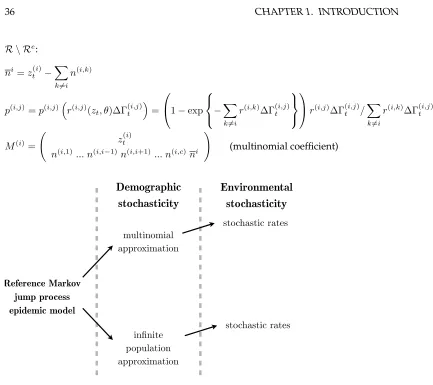
Reference Markov jump process epidemic model

multinomial approximation

infinite population approximation

stochastic rates

Demographic

stochasticity

Environmental

stochasticity

Tuesday, February 19, 13

Figure 1.1: Representation of the different epidemic models introduced in the thesis

Again, the authors of Breto et al. (2009) have proved that this infinitesimal generator characterises a properly defined Markov chain in the limitδ→0. Alternatively, environ-mental noise can also be introduced in the infinite population setting, defining a stochastic differential equation driven by Gamma noise:

Epidemic model with stochastic rates under infinite population approximation

dz˙t= X

(i,j)∈Re

k(i,j)r˙(i,j)( ˙zt)dΓ(i,j)+ X

(i,j)∈R\Re

Variations in climate and human behaviour, however, cannot always be modelled as white noise as they have been shown to exhibit complex seasonal and inter-annual patterns (Meehl, 1987) influencing epidemic dynamics (Viboud et al., 2004). We explore in this thesis an alternative description of environmental noise by allowing certain parameters to vary in time in order to capture the influence of time-varying drivers of epidemics. A graphical representation of the different mathematical formulations of epidemic models that have just been introduced is provided in Figure 1.1. When the sizeNof the population tends to infinity, it is expected that the models based on the multinomial approximations converge to the ones defined under the infinite population approximation. A complete theoretical study of the nature of this convergence, however, has not yet been contributed to the literature to our knowledge.

Modelling observation regimes

Observation regimes of epidemics can take a variety of forms. Examples of data used to study their course are incidence, prevalence, and death counts. A substantial amount of uncertainty is generally associated with the collection of such data, principally due to the following reasons:

non-report: depending on disease severity, there can be a substantial proportion of individ-uals that do not consult a doctor, which leads to unrecorded cases.

asymptomatics: a proportion of the individuals infected with a disease will be infectious without developping any symptom. For influenza, virus inoculation to voluntary individuals have revealed that the proportion of asymptomatics could vary between 25% and 40% (Carrat et al., 2008).

false positives: different diseases can induce similar symptoms, which leads to uncertainties in diagnosis records. For example, it has been estimated that only 40% of patients that consult doctors for influenza-like symptoms are truly infected with influenza (Finkenstadt et al., 2005).

A general model for incidence data is the binomial distribution. The number of recorded cases on weekiis denoted byyi,αaccounts for the rate of false positives andρis the

re-porting rate (which incorporates asymptomatics). Under these notations, the probability of recordingyinew cases over weeki, ifInciis the true number of new infections having

occurred over the same week, is given byBinom((1−α)yi, Inci, ρ). In theSEIRmodel,

for example, incidence is defined asR

kEtdt: cases can only be detected after the onset of

preserve the Markovianity of the model and of the observation process, an artificial addi-tional component can be added to the state vector to account for the accumulation of new cases over an observation period. For example, the state vector for an SEIR model that will be observed through incidence can be formulated as{St, Et, It, Rt, Inct}.

1.2

Bayesian inference for indirectly observed stochastic processes

In this section, we propose a general formulation for indirectly observed stochastic pro-cesses, and present a series of notions that will serve as a basis for further development along the thesis. The problem we address is the efficient exploration of the joint poste-rior densityp(x0:n, θ|y0:n), wherex0:n is the path of the driving stochastic process, andθ

is a vector of constant parameters playing a role in the dynamic and observation of the system. More precisely, we will see that for any statistic that needs to be computed from the target density p(x0:n, θ|y0:n), unbiased estimates relying on an approximate density

pδ(xdis0:n, θ|y0:n)based on a time discretisation with resolutionδcan be obtained up to Monte

Carlo error. If the inference algorithm is robust to refinements of the resolutionδ, both the bias due to discretisation and the variability induced by Monte Carlo error can always be reduced by increasing the computation time. Inference methods for which these sources of error can be rendered negligible will be calledasymptotically exactin this thesis: in such cases, the hypothetical facts derived from the confrontation of a model to a given dataset are intrinsic to the model. Thus, models can be tested and compared, independently of the utilised inference algorithms.

Lastly, there appears to be a gap between the models and methods that are being used by practitioners to design and evaluate public health interventions, and the models and methods that have been appearing in the literature in the recent years (Brisson and Ed-munds, 2006). This observation has motivated the development of plug-and-play algo-rithms; in this perspective, ease of use and automatic calibration will be central concerns in this thesis.

1.2.1

General framework for indirectly observed stochastic processes

We are interested in studying the paths and parameters of underlying stochastic processes that deterministically drive the trajectory of discretely observed auxiliary variables ob-served with noise. The driving process will be notedxt. The auxiliary or complementary

components, denotedzt, are generally needed to obtain a complete description of the

sys-tem and bridge the gap between the process of interest and the available observations of the system. The concatenation of vectorsxtandztform the state vectorwt={xt, zt}. We

or integer-valued. We notex0:n andz0:n the corresponding trajectories between timest0

andtn. More generally, state variables with subscriptiwill be an abuse of notation for

their value at timeti. The model can then be defined in the following way:         

x0:n∼p(.|θ)

z0:n=f(x0:n, θ)

p(yi|zi, θ) =ht(zi, θ)

(1.7)

This general formulation encompasses all the problems explored in this thesis. It nat-urally includes the case of directly observed stochastic processes, by settingzt = xt,

al-though in that case specific solutions may be more efficient than the ones explored in this thesis. An assumption often made in this context imposes the Markov property onwt.

Markovian state-space model can simply be defined through their instantaneous dynamic and the observation process:

        

xt+δ ∼p(.|xt, zt, θ)

zt+δ ∼f(zt, xt, θ)

p(yi|zti, xti) =ht(zti, θ)

(1.8)

Note that we make the potential interaction between zt and xt explicit in 1.8, aszt

may carry information about past values of the driving stochastic process. We will now give examples of such processes, starting with the general formulations of compartmental epidemic models introduced in the previous Section.

Compartmental epidemic models

We illustrate here how the different epidemic models that have been introduced in the pre-vious section (see Figure 1.1) can be formulated as indirectly observed stochastic processes. The simplest stochastic model is defined under the infinite population approximation by introducing environmental stochasticity through stochastic rates. Noise increments can be contained in a vectornxΓ(i,j)_{,(i, j)∈ R}eo_{, withR}e_{⊂ Rcontaining the indexes of reactions}

with stochastic rates:

        

x_tΓ(i,j) =dΓ_t(i,j) for(i, j)∈ Re

dz˙t= X

(i,j)∈Re

k(i,j)r˙(i,j)( ˙zt, θ)xΓ

(i,j)

t +

X

(i,j)∈R\Re

For illustration, we also provide the formulation of epidemic models with stochastic rates under the multinomial approximation in the indirectly observed stochastic process framework. It additionally involvesxN(i,j)

t , which denotes the total number of times

reac-tion(i, j)has occurred up to timet:

                    

xΓ_t(i,j) =dΓ_t(i,j) for(i, j)∈ Re _(xΓ(i,j)

t ≡δ if (i, j)∈ R \ Re)

p(xN_t+(i,j_δ )=x_tN(i,j)+n(i,j)|xN

(i,j)

t , x

Γ(i,j)

t , zt) =E    c Y i=1     

M(i) 

1−

X

k6=i

p(i,k) 

 ni

Y

j6=i

p(i,j)

n(i,j)        +o(δ)

zt+δ=zt+ X

(i,j)∈R

k(i,j)xN_t (i,j)

We use the following notations, withr(i,j)_{≡0if(i, j)∈ R/ :}

ni=zt(i)− X

k6=i

n(i,k)

p(_ti,j)=p(i,j)r(i,j)(zt, θ)xΓ

(i,j)

t

= 1−exp

(

−X

k

r(i,k)xΓ_t(i,j) )!

r(i,j)xΓ_t(i,j)/X

k

r(i,k)xΓ_t(i,j)

M(i)= z

(i)

t

n(i,1)_{... n}(i,i−1)_n(i,i+1)_{... n}(i,c)_ni !

(multinomial coefficient)

Hypoelliptic diffusions

Diffusion processes, that are a classic example of stochastic processes, will be recurrent along this thesis. They correspond to the solutions of stochastic differential equations writ-ten in the following manner:

dwt=µt(wt, θ)dt+LdBtQ(wt, θ) (1.9)

The matrixLis referred to as a dispersion matrix, anddBQ_t is a Brownian motion with diffusion matrix Q. This formalism, is also used in Särkkä (2006), and allows the flexible introduction of various types of correlated and uncorrelated noise that will be explored in Chapter 2. Hypoelliptic diffusions correspond to cases where the matrixLQLT is degen-erate. Without loss of generality, these systems can all be reformulated under the Marko-vian indirectly observed stochastic processes framework (Eq 1.8), withL˜Q˜L˜T _being

non-singular:







dxt=µxt(xt, θ)dt+ ˜LdB

˜

Q t (wt, θ)

dzt=f(zt, xt, θ) =µzt(xt, ztθ)dt

Integrated Brownian Motion

The Integrated Brownian motion (IBM) will be utilised in this thesis as a way to derive a differentiable path from a diffusing object. It can be simply defined in the following manner:







dxt=σdBt

dzt+δt=xtdt

(1.11)

Volatility models and extensions thereof

The Stochastic Volatility models, ubiquitous in financial applications, are a classic example of indirectly observed diffusion processes formulated as stochastic differential equations. They model the priceutof an asset as a diffusion process which volatility term is driven by

a quantityvtthat is also stochastic and follows a diffusion process. Prices are considered to

be exactly observed at discrete times(ti)i=1:n, defining an observation vector(yi)i=1:n. A

general class of Stochastic Volatility models can be written in the following way (Heston, 1993), withdB_t(1)anddB_t(2)being independent Brownian motion increments:



   

   

dut= (µu−σv(vt)2/2)dt+σu(vt)dB

(1)

t

dvt=κ(µv−vt)dt+σvdB

(2)

t

yi=uti

(1.12)

They can be put in our indirectly observed diffusions framework:



    

    

dxt=κ(µv−xt)dt+σvdBt

zt= Z t

ti−1

σv(xs)2ds

yi =N(yi−1+µu(ti−ti−1)−zti/2, zti)

(1.13)

In Chapter 4, we will develop efficient inference methods for fractional versions of the stochastic volatility models, where the stochastic volatility is driven by non-independent fractional Brownian motion increments.

1.2.2

Simulation schemes

the discretisation time step tends to 0, it is expected that the probability densities implied by the discretised models converge to the one of the continuous-time model. The valid-ity of this convergence result, as well as the nature and speed of convergence, will vary depending on the model and discretisation scheme.

Simulating paths of stochastic differential equations

One of the simplest ways to sample from a stochastic differential equation, whether it is hypoelliptic or not, is the Euler-Maruyama algorithm (Kloeden and Platen, 1999; Särkkä, 2006). The strong convergence of this algorithm is of orderO(δ1/2_{), but as in the}

determin-istic setting Runge-Kutta algorithms allow for higher orders of convergence. Algorithm 1Euler-Maruyama algorithm: sampling from an SDE (Eq. 1.9)

Initialisex0,t= 0

whilet<Tdo

DrawεfromN(0, Q(t)δ) wdis

t+δ =wdist +µ(wdist , θ)δ+Lε

t=t+δ

end while

Simulating from the reference Markov jump process epidemic model

Doob and Gillespie have explored means to generate exact simulations from the Markov jump process epidemic model of Eq. 1.2 (Doob, 1942, 1945; Gillespie, 1977). Given the state

ztof the system at a timet, the Doob-Gillespie algorithm relies on the simple probability

distribution of the following event:

"no reaction occurs during[t;t+τ[and reactionihappens at timet+τ"

Algorithm 2 follows, for the exact exploration ofp(xt|θ)in continuous time. However,

its computational cost increases exponentially with the size of the population, through the necessary decrease of time incrementsτ. Alternative means to simulate from the Markov jump processes used in epidemiology have been explored. Gillespie, again, proposed a

τ−leapalgorihtm that serves as a basis for the multinomial approximation introduced in Breto et al. (2009).

Simulating epidemics through multinomial processes

Algorithm 2Doobs-Gillespie algorithm Initialisez(0),t= 0

whilet<Tdo

Sample a lagτwithp(τ) =P

(i,j)∈Rr

(i,j)_(z

t, θ)

exp−τP

(i,j)∈Rr

(i,j)_(z

t, θ)

Sample a reaction(i, j)knowing thatp(i,j)_=r(i,j)_(z

t, θ)/P_(k,l)∈Rr(k,l)(zt, θ)

z(t+τ) =z(t) +ki

t=