Study of Work Travel Related Behavior Using Principal Component Analysis

http://dx.doi.org/10.4236/ojs.2014.411084

Study of Work-Travel Related Behavior

Using Principal Component Analysis

Cira Souza Pitombo, Monique Martins Gomes

Department of Transportation Engineering, University of São Paulo, São Carlos, Brazil Email: [email protected], [email protected]

Received 26 September 2014; revised 20 October 2014; accepted 8 November 2014

Copyright © 2014 by authors and Scientific Research Publishing Inc.

This work is licensed under the Creative Commons Attribution International License (CC BY). http://creativecommons.org/licenses/by/4.0/

Abstract

The main objective of this study is to analyze work travel-related behavior through a set of va-riables relative to socio-economic class, urban environment and travel characteristics. The Prin-cipal Component Analysis was applied in a sample consisting of workers of the São Paulo Metro-politan Area, based on the origin-destination home interview survey, carried out in 1997, in order to: 1) examine the interdependence between travel patterns and a set of socioeconomic and urban environment variables; 2) determine if the original database can be synthetized on components. The results enabled to observe relations between the individual’s socio-economic class and car usage, characteristics of urban environment and destination choices, as well as age and non-mo- torized travel mode choice. It is then concluded that the database can be adequately summarized in three components for subsequent analysis: 1) urban environment; 2) socio-economic class; and 3) family structure.

Keywords

Travel Behavior, Principal Component Analysis, Exploratory Analysis

1. Introduction

Personal displacement behavior depends largely on two groups of variables: socioeconomic characteristics, and urban environment factors (residential density, proximity of localities, spatial coverage of the transportation net- work, etc.).

The influence of individual socioeconomic and household characteristics on choosing travel patterns has been studied over the years [1]. The affirmation that personal displacement behavior can be determined by gender, car ownership, the individual household role, and tasks allocation is widely seen in the literature [2] [3].

va-riables that individuals take in account when making their travel decisions (travel mode choices, destination, route, etc.). Urban densities, city shape, more or less dispersed activities in the urban environment, for example, are strongly related to the modal choice.

The main objective is to analyze, through exploratory techniques, the individual work-travel behavior through a set of variables related to socioeconomic characteristics and to the urban environment (distribution and inten-sity of opportunities).

The Principal Component Analysis (PCA) was applied to a sample of workers of the São Paulo Metropolitan Area (SPMA) in order to: 1) examine patterns or relations a priori unknown between travels and a large set of variables; 2) determine if the original database can be synthesized in a set of components.

2. Study of Hypothesis

This paper analyzes the interdependence between a set of variables and work-related travel behavior. A sequence of steps was performed to examine three main hypotheses: 1) if characteristics related to the individual’s so-cio-economic class affect the modal choice and travel distances; 2) if variables related to the family structure af-fect the travel behavior; 3) if distribution and intensity of opportunities in the urban environment have efaf-fect on destination choice decisions.

3. Paper Structure

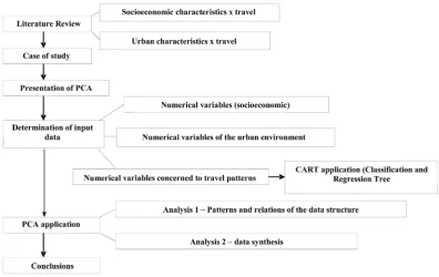
This paper is organized into sections and subsections according to the methodological framework presented in Figure 1.

4. Socioeconomic Characteristics and Travel Patterns

In general, socioeconomic characteristics are strongly related to human behavior. Some attributes (such as in-come) provide an appropriate base for population segmentation and comprehension of individual behavior, par-ticularly travel behavior.

Travel pattern choices are strongly related to the individual’s socio-economic class, traditional division of household roles and family structure [4]-[6]. These two groups of variables have often been included in the study of urban travel behavior.

A broad range of household characteristics influence the complexity of trip chains including age, income, gender. Like household characteristics, travel patterns such as origin, destination, purpose, characteristics of transportation system and the number of vehicles per household also influence trip chain behavior [7]-[9]. This will be discussed in more details in the next subsection.

4.1. Socio-Economic Class

Hanson and Hanson [10] consider the individuals’ type of occupation, as well as their level of education, income and car ownership, the standard variables that feature the socioeconomic status or class. This group of variables affects travel behavior, particularly in relation to the travel mode and travel distance.

Mitchell and Town [11] used the variable: individual’s occupation, as standard of social status. The authors concluded that better jobs are associated with an increase in the proportion of car travels and a decrease in public transportation or non-motorized travels. Clearly car ownership affects travel behavior. Individuals who have a car in their residence travel more in general, whether for shopping-related trips or for other travel purposes [12]. Higher-income individuals travel more per day, more social travels and travel longer distances.

Kitamura [13] analyzed relations between characteristics of trip chaining (including the average distance tra-veled and chaining trip tendency) and parameters characterizing a linear city and socioeconomic characteristics. The author observed that high-income individuals, whose travel cost evaluations are supposedly smaller, tend to make longer trips.

Dargay [14] shows that long distance travel is strongly related to income: air is most income-elastic, followed by rail, car and finally coach. This is the case for most long distance journey purposes.

4.2. Household Roles and Family Structure

The household structure and family size also can influence travel patterns. Travel is part of a structure of house-hold activities. The division of househouse-hold tasks, influenced mostly by the individual’s family role (family heads, spouse, etc.) is fundamental, considering the differences found on the travel patterns performed by the family members. Women classified as non-spouse and non-family heads, represent higher number of work-commuters. On the other hand, women classified as spouse or family heads represent lower rates of work-commuters [2].

Lee et al. [15] used the entire sample and a sub-sample of worker households from Tucson’s Household Tra-vel Survey and two sets of models are deTra-veloped to better understand the phenomena of trip-chaining behavior among five types of households: single non-worker households, single worker households, couple non-worker households, couple one-worker households, and couple two-worker households. Therefore, durations of out-of- home subsistence, maintenance, and discretionary activities within trip chains are examined. Factors found to be associated with trip-chaining behavior include intra-household interactions with the household types and their structure and household head attributes.

5. Urban Environment Characteristics and Travel Patterns

Considering the relation between urban density and travel behavior, Newman and Kenworthy [16] compare dif-ferent cities in the world with difdif-ferent population densities, and their travel behavior. The authors concluded that cities with higher population densities are less dependent on cars than lower density cities. Cervero and Ra-disch [17] concluded that individuals who live in more compacted regions with mixed land use and pedestrian facilities normally perform non-motorized travel mode or transit trips, when compared to those who live in typ-ical North American suburbs.

Handy [18] asserts that high levels of accessibility affect non work trips. Aditjandra et al. [19] explored whether changes in neighborhood characteristics bring about travel choice changes. The case study is based on the Metropolitan Area of Tyne and Wear, North East of England, UK. The results identified that neighborhood characteristics do influence travel behavior after controlling for self-selection. For instance, the more people are exposed to transit access, the more likely they are to drive less. Neighborhood characteristics also influence car ownership. A social environment with vitality also reduces the amount of private car travel.

6. Case of Study

Metropolitan Area (SPMA) in 1997. At that time, SPMA’s population was of approximately 17 million, distri-buted in 39 counties and 389 traffic zones. The interview survey included socioeconomic and travel characteris-tics data. Originally, the SPMA database is composed of 98,780 individuals.

The data processing phase includes the following steps: 1) removal of incomplete data; 2) omission of indi-viduals who do not work; 3) removal of indiindi-viduals who do not work at industrial, commercial or service sectors; 4) omission of individuals who did not travel the day before the interview survey. Thus, a sample of workers in the industrial, commercial and service sector was obtained, composed of 24,335 individuals.

7. Principal Component Analysis

Principal Components Analysis (PCA) is an exploratory multivariate data analysis technique whose main objec-tive is to detect the structure of a large set of variables (data patterns and relations) and to reduce multidimen-sional data sets to lower dimensions.

From the dependence structure between the variables in question, the PCA enables the creation of a lower set of variables (factors or components) obtained according to the original variables. Additionally, it is possible to know to what extent each component is associated with each variable and how much the set of components ex-plains the variability of the original data.

PCA is a technique of interdependence and analyzes the mutual association between all numeric variables. The use of PCA is mainly recommended in studies of multiple variables with high inter-correlation. Its applica-tion can be used to solve multicollinearity problems as the factor is a combinaapplica-tion of variables, which are inter- orthogonal [20] [21].

One of the main advantages of PCA is that there is no presupposition of normality of the variables involved. The components are obtained from a decomposition of the correlation matrix. The factorial loads are the result of this decomposition, which indicate how much each variable is associated with each one of the factors in-volved.

The eigenvalues are numbers that reflect the importance of the factor. When the number of factors is the same as the number of variables, the sum of eigenvalues corresponds to the sum of the variance of these variables. The factorial loads are parameters which express the covariance between each factor and the original variables. When standardized variables are used (correlation matrix), these values correspond to the correlation between the factor and the original variables.

Hence, PCA can: 1) identify the structure or relations between variables by analyzing the correlation between variables (Analysis 1 of this paper); 2) create a new and lower set of variables (factors/components) that can re-place partially or totally the original one for application of the following techniques (Analysis 2 of this paper). There are four steps to using PCA, described as follows.

1) Calculate the correlation matrix of the variables under study―verify the level of association of the va-riables among themselves;

2) Extract the more significant components that explain as much information as possible (maximum variabil-ity data―eigenvalues should usually be equal to or greater than 1;

3) Understand and name each factor, observing the contribution (factorial load) of all the variables; 4) Factorial load generation (for each individual) to be used in other analyses.

8. Input Variables―Socioeconomic Variables

At this stage, the variables that are interrelated with the travel patterns were selected. The variables related to the socioeconomic characteristics were chosen through current literature and data availability. As mentioned before, PCA allows the use only of numeric variables. Thus, through the original data base the variables were selected and adapted as shown in Table 1.

9. Input Variables―Urban Environment

Table 1. Socioeconomic variables selected from database.

Socioeconomic variables

FAM Number of family members AGE Age

CAR Number of cars in the household II Individual income

FI Family income (R$) NCH Number of children at the household

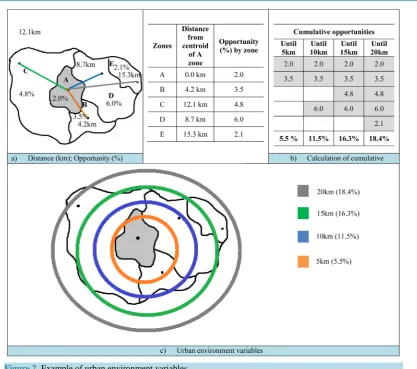
What is the meaning of level of “cumulative opportunity”? In this paper, opportunity refers to the job offer (industry, commerce and services). Hence, the term “opportunity” represents a “proportion” (%) of total of em-ployment.

Then, this proportion of jobs was accumulated by distance buffers, considered between the centroids of the residence area to the centroids of the zones located at : 5 km, 10 km, 15 km and 20 km, thus generating the term: “cumulative opportunity”.

Figure 2 exemplifies the proposal of variables for the urban environment. The origin zone is the central “A” (shaded). At this stage 1), the values of the “opportunities” in (%) for each zone are represented as distances straight from the centroid of “A”. In stage 2) the calculation for the “cumulative opportunities” for each one of the four buffer distance is shown. Finally, in stage 3) the urban environment variables proposed from traffic zone A are illustrated.

10. Input Variables―Travel Patterns

The input variables related to travel behavior took into account the main trips performed by individuals the day before the home interview survey. Main trips are those in which remained for a longer period in its destination. Most of the travels performed were work-related trips.

Therefore, main travels were characterized by their purpose, travel mode, and distance traveled. In this paper, three travel purposes were considered: 1) WORK―work industry, commerce, or services; 2) SCH―school; and 3) ACT―other activities. For travel modes, three different categories were analyzed: 1) CAR―private moto-rized travel mode; 2) PUB―transit; 3) NM―non-motorized travel mode.

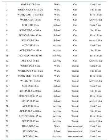
Finally, the traveled distances were clustered in 4 groups: 5 km―for less than 5 km; 2) 5 to 10 km―between 5 and 10 km; 3) 10 to 15 km―between 10 and 15 km; and 4) 15 km―more than 15 km. By grouping the three travel attributes, each category indicated a purpose, the travel mode, and the travel distance, simultaneously. Ta- ble 2 shows all the categories considered in this paper.

However, there is an important question to be discussed. How to measure numerically each one of the catego-ries since the PCA is a technique which allows only the use of numeric variables? Thus, applying the CART al-gorithm (Classification and Regression Tree, described in the next section), the probability of each worker per-forming each of the 27 travel categories was calculated. The next subsection describes CART algorithm, its use in the paper, thus the conversion of a categorical variable to a numeric variable.

Use of CART―Auxiliary Tool

In this paper a variant of the CART algorithm contained in the SPSS 19.0 software was used as an auxiliary tool. CART establishes a relationship within independent and dependent variables. The algorithm is adjusted by suc-cessive binary splitting in the data set, and so the resulting subsets are increasingly more homogeneous in rela-tion to the dependent variable. These divisions are represented by a binary tree structure, and each node corres-ponds to a splitting [22].

CART is an exploratory technique and can be defined as an acyclic graph that satisfies the following proper-ties: 1) the hierarchy is called tree and each segment is known as a node; 2) there is a node, called root node, which contains the complete database; 3) the root node is divided sequentially, generating child nodes; 4) there is only one path within the root node and each node; 5) when no further data subdivision is possible, the final subgroups are considered terminal nodes or leaves; 6) for construction of the CART, three main elements should be determined: a set of questions delimiting data division, a criterion for evaluating the best division and a rule for the conclusion of the other subdivisions (stop-splitting rule).

Figure 2. Example of urban environment variables.

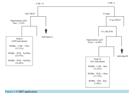
undertake each of the 27 travel categories represented in Table 2. Thus, from the worker sample, 27 categories of dependent variables (travel related variables) and independent numerical and categorical variables (socioeco-nomic and urban environment variables), the tree was generated with a minimum deviation of 0.5 (stop splitting rule), resulting in 8 leaves. To represent the travel variables as continuous variables, with values between zero and one-of likelihood, the following examples are considered.

1) Individual A is observed; 2) with the application of the CART algorithm, individual A is classified in node 8; 3) the individuals that compose leaf 8 have a 31.31% probability to perform the category of TRAB-PUB-15 km, for example; 4) the probability of performing the TRAB-PUB-15 km (0.3131) is the value of the variable called “TRAB-PUB-15 km” for the individual A; Thus, each one of the 27 categories is associated to a numeric number that corresponds to the probability an individual will perform the specified travel characteristic. The following values are observed for individual A: TRAB-PUB-5 to 10 km (0.2197); TRAB-PUB-10 to 15 km (0.1644).

For the individual B, for example, the variable TRAB-PUB-15 km assumes the value of 0.1175. The variable TRAB-AUT-5 km assumes the value 0.1235, whereas the value of the variable TRAB-NM-5 km is 0.1096. Figure 3 shows only three categories for frequent travel patterns on leaves 8 and 52, respectively. However, through the CART application, the probabilities of all 27 categories occurring in all leaves were calculated, thus, for all individuals in the sample.

11. Principal Component Analysis Application―Analysis 1

Table 2. Variables related to travel.

1 WORK-CAR-5 km Work Car Until 5 km

2 WORK-CAR-5 to 10 km Work Car 5 to 10 km

3 WORK-CAR-10 to 15 km Work Car 10 to 15 km

4 WORK-CAR-15 km Work Car Above 15 km

5 SCH-CAR-5 km School Car Until 5 km

6 SCH-CAR-5 to 10 km School Car 5 to 10 km

7 SCH-CAR-10 to 15 km School Car 10 to 15 km

8 SCH-CAR-15 km School Car Above 15 km

9 ACT-CAR-5 km Activity Car Until 5 km

10 ACT-CAR-5 to 10 km Activity Car 5 to 10 km

11 ACT-CAR-10 to 15 km Activity Car 10 to 15 km

12 ACT-CAR-15 km Activity Car Above 15 km

13 WORK-PUB-5 km Work Transit Until 5 km

14 WORK-PUB-5 to 10 km Work Transit 5 to 10 km

15 WORK-PUB-10 to 15 km Work Transit 10 to 15 km

16 WORK-PUB-15 km Work Transit Above 15 km

17 SCH-PUB-5 km School Transit Until 5 km

18 SCH-PUB-5 to 10 km School Transit 5 to 10 km

19 SCH-PUB-10 to 15 km School Transit 10 to 15 km

20 SCH-PUB-15 km School Transit Above 15 km

21 ACT-PUB-5 km Activity Transit Until 5 km

22 ACT-PUB-5 to 10 km Activity Transit 5 to 10 km

23 ACT-PUB-10 to 15 km Activity Transit 10 to 15 km

24 ACT-PUB-15 km Activity Transit Above 15 km

25 TRAB-NM-5 km Work Non-motorized Until 5 km

26 SCH-NM-5 km School Non-motorized Until 5 km

27 ACT-NM-5 km Activity Non-motorized Until 5 km

A) six socioeconomic variables (FAM―number of individuals in the family, CAR―number of cars per household, RF―family income, AGE―age, II―individual income, NCH―number of children per household); B) four urban environment variables (until 5 km―cumulative opportunities until 5 km; until 10 km―cumuli- tive opportunities until 10 km; until 15 km―cumulative opportunities until 15 km; until 20 km―cumulative opportunities until 20 km); C) twenty two variables related to travel patterns (likelihood to perform 22 of 27 categories described in Table 2). Five school travel categories were excluded: SCH-CAR-5 to 10 km: SCH- CAR-10 to 15 km; SCH-PUB-5 to 10 km; SCH-PUB-10 to 15 km; SCH-PUB-15 km. For PCA application, the four steps described in section 7 were considered.

11.1. Calculation of the Correlation Matrix of Variables under Study

Figure 3. CART application.

The higher correlation values were found for the variables related to urban environment (this was expected as these variables are cumulative). The same variables are inversely correlated to the categories ACT-PUB-15 km and WORK-PUB-15 km. This kind of inverse correlation makes sense because if there are high values of op-portunities at the neighborhood, there will be a lower probability of individuals performing long trips (15 kilo-meters or more), mainly to work.

Family income and car ownership are also highly correlated variables. They are also correlated to travel cate-gories related to car usage. The correlation matrix gives an idea of the general structure of the data and of the existing relations.

11.2. Extraction of the Most Significant Factors

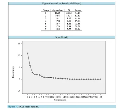
The initial factor extraction criteria were eigenvalues greater than one (latent root criterion). Thus, seven com-ponents were extracted, with 83% of variability explained from the original data. Thus, the 32 initial variables can be explained by the seven components. Figure 4 represents the values of eigenvalues, percentage of varia-bility explained in each component and the scree plot, respectively.

11.3. Interpretation of Each Factor

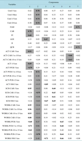
To properly interpret and also name the factors or components, it is necessary to analyze the factorial load values of the variables. The factorial loads are the contribution (negative or positive) analyzed for each of the variables related to each of the seven components. Table 3 shows the variables and the factorial load values for each component. Following, the results will be discussed and nomenclatures will be used for all factors.

Component 1: individual’s socio-economic class

The first component should be the most important as it explains about 32% of the variability for the total data. High and positive factorial loads were observed for the variable CAR (number of cars at the household) and FI (familiar income).

Figure 4. PCA main results.

of travel categories of car usage, regardless of the travel purpose, as well as distance traveled. Also negative work trip values performed by public transportation were observed. It can be stated that Component 1 represents the individual socio-economic class that is strongly associated to the travel mode choice, especially to car usage.

Component 2: urban environment

The second component explains about 18% of data variability, especially characterizes the urban environment. There were high and positive values for the four variables related to the urban environment (cumulative oppor-tunities by buffer distance).

How is the urban environment factor associated to travel behavior? In the literature predominates the state-ment that compact cities with well distributed mixed activities (high density) benefit from the use of non-moto- rized travel mode or lower distance travels. According to factorial loads observed in component 2, high and neg-ative values for distances higher than 15 km are verified, in other words, the greater the number of cumulneg-ative opportunities, the lower the probability of individuals travelling more than 15 km to satisfy their travel purpose.

Component 3: age vs. non-motorized travel mode

Component 3 explains about 9% of the data, and it has a high and positive factorial load value for the age va-riable. However, high and negative values for categories related to non-motorized travel mode and travel dis-tance lower than 5km were observed. Intuitively it is expected that older individuals have more travelling re-strictions with the non-motorized travel mode, mainly when distances are longer than 1km, for example.

Component 4: school

Component 4 is associated with school travel categories. The variables related to these activities (mainly in-volved with study) would probably have high contributions to the referred factor.

Component 5: work

Table 3. Factorial loads.

Variables

Components

1 2 3 4 5 6 7

Until 5 km 0.42 0.70 0.00 0.37 0.27 0.05 0.08

Until 10km 0.41 0.75 0.04 0.33 0.33 0.03 0.08

Until 15 km 0.41 0.74 0.06 0.30 0.36 0.02 0.08

Until 20 km 0.38 0.74 0.07 0.26 0.37 0.00 0.08

FAM −0.24 −0.02 −0.08 −0.12 −0.13 −0.02 0.71

CAR 0.78 −0.19 −0.04 −0.13 0.23 0.14 0.01

FI 0.68 0.01 0.04 −0.18 0.05 0.38 0.06

AGE 0.33 0.05 0.65 0.12 −0.24 −0.07 −0.32

II 0.48 0.02 0.23 −0.08 −0.19 0.37 −0.02

QCR −0.17 −0.06 0.06 −0.01 −0.24 −0.12 0.72

ACT-CAR-5 km 0.92 −0.17 0.02 0.04 0.05 0.10 0.09

ACT-CAR-5 to 10 km 0.27 −0.54 0.14 0.33 −0.02 −0.66 −0.02

ACT-CAR-10 to 15 km 0.49 −0.49 −0.05 0.21 0.19 −0.63 0.06

ACT-15 km 0.69 −0.24 0.13 −0.02 −0.06 0.49 0.11

ACT-PUB-5 km −0.79 0.29 −0.04 0.21 −0.15 0.09 −0.02

ACT-PUB-5 to 10 km −0.34 0.72 0.15 0.23 0.44 −0.04 −0.01

ACT-PUB-10 to 15 km 0.01 0.38 0.41 −0.37 −0.01 −0.28 0.00

ACT-PUB-15 km −0.58 −0.58 −0.01 −0.05 0.03 0.16 −0.05

ACT-NM-5 km 0.00 −0.15 −0.85 −0.09 0.19 −0.04 0.02

SCH-CAR-5 km 0.95 −0.12 0.08 0.60 −0.11 −0.23 0.01

SCH-CAR-15 km −0.16 −0.75 0.22 0.65 0.05 −0.04 0.05

SCH-PUB-5 km −0.30 −0.58 −0.18 0.61 0.27 0.42 0.03

SCH-NM-5 km −0.16 −0.03 −0.67 0.69 0.51 −0.08 −0.02

WORK-CAR-5 km 0.95 −0.14 −0.05 −0.07 0.02 −0.23 0.01

WORK-CAR-5 to 10 km 0.96 −0.15 0.01 −0.14 0.03 −0.06 0.03

WORK-CAR-10 to 15 km 0.93 −0.11 0.05 −0.08 0.02 0.02 −0.01

WORK-CAR-15 km 0.88 −0.10 0.19 −0.02 −0.24 0.25 0.01

WORK-PUB-5 km −0.60 0.47 0.34 −0.02 0.65 −0.06 0.05

WORK-PUB-5 to 10 km −0.71 0.06 0.51 −0.26 0.68 −0.05 0.01

WORK-PUB-10 to 15 km −0.62 −0.20 0.52 −0.20 0.40 0.04 0.02

WORK-PUB-15 km −0.51 −0.70 0.21 0.29 0.64 0.19 0.05

WORK-NM-5 km −0.29 0.46 −0.71 0.12 0.66 0.00 −0.08

Component 6: other activities

Finally, component 7 is characterized by FAM variables (number of individuals in the family) and NCH (number of children per household). There is no contribution associated to any travel category. As it is consi-dered the main travel, a strong relationship between family structure and travel behavior cannot be expected. Perhaps stronger relations could be found for the complexity of trip chaining, for example. Number of children can be associated to the number of travels per day. The higher the number of children, the higher the number of trips performed, per day.

12. Principal Component Analysis Application―Analysis 2

The purpose of the second analysis applying PCA is to determine whether the original database can be synthe-sized in a set of factors/components. The dataset obtained can be used on subsequent analyses, especially using techniques that analyze the dependence between variables and suppose that there are no correlations within the independent variables.

In analysis 2, the variables related to travel pattern categories were excluded. Only socioeconomic and urban environment numerical variables were used, totalizing ten variables.

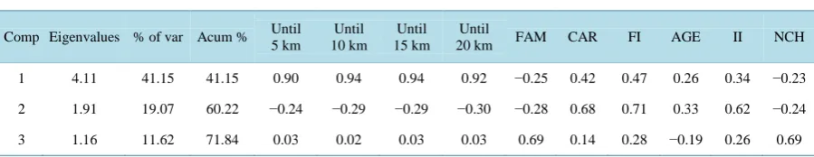
The latent root criterion was also used to extract the components. Next, three components with “approximate explanation” of 72% of data variability were obtained. Table 4 summarizes the results obtained.

According to factorial load values, the three obtained components can be termed: 1) component 1: urban en-vironment; 2) component 2: individual socio-economic class; 3) component 3: family structure. The ten va-riables can be synthesized in three components that represent the attributes which supposedly influence travel behavior. Then, the individual factorial load of these three components can be used on sequential analyses, espe-cially when applying techniques where there are restrictions related to multicollinearity.

13. Conclusions

Through an exploratory analysis, this work seeks to better understand the factor that individuals (mainly workers) consider when choosing travel modes, distances and purposes. The components found are adequate to synthesize the data set in three factors which characterize (also according to the literature reviewed) the characteristics that influence travel behavior: 1) socio-economic class; 2) family structure; and 3) urban environment.

Analyzing the data structure (PCA application―analysis 1), in order to examine patterns or relations between travel variables and a large data set, enabled supporting the main hypothesis of this work.

Hypothesis 1: socio-economic class affects the modal choice and travel distances

Applying PCA in the first analysis, through component 1 the relation between socio-economic class (CAR and II), and travel behavior was observed. The higher the income or number of cars in the household, the higher the probability of choosing the car, thus lower the probability of using non-motorized travel mode or transit.

Hypothesis 2: variables related to the family structure affect travel behavior

Component 7 (analysis 1 of PCA), which features the family structure, had no apparent relationship with vel behavior. However, the family structure can influence the complexity of trip-chaining, or the number of tra-vels performed, but not the main travel, which was represented in this paper.

Hypothesis 3: distribution and intensity of opportunities in the urban environment affect the destina-tion choices.

Through component 2 (analysis 1 of PCA), one can concluded that the higher the number of cumulative op-portunities in the residence zone, the lower the probability of individuals making long trips. Work trips, which are often scheduled with fixed locations, can affect the long term choices. Particularly in the São Paulo Metro-politan Area, many individuals choose to live close to their work locations, especially in regions with high

Table 4. Results of principal component analysis―analysis 2.

Comp Eigenvalues % of var Acum % Until 5 km Until 10 km Until 15 km Until

20 km FAM CAR FI AGE II NCH

1 4.11 41.15 41.15 0.90 0.94 0.94 0.92 −0.25 0.42 0.47 0.26 0.34 −0.23

2 1.91 19.07 60.22 −0.24 −0.29 −0.29 −0.30 −0.28 0.68 0.71 0.33 0.62 −0.24

numbers of job offers.

Acknowledgements

This work was supported by the Conselho Nacional de Desenvolvimento Científico and Tecnológico (CNPQ). We also acknowledge the São Paulo Metro for providing the data.

References

[1] Lu, X. and Pas, I. (1998) Socio-Demographics, Activity Participation and Travel Behavior. Transportation Research Part A, 33, 1-18. http://dx.doi.org/10.1016/S0965-8564(98)00020-2

[2] Strambi, O., Vespucci, K.M. and Van de Bilt, K. (2004) Analysis of the Evolution of Classes of Individual Patterns and Their Relation to Socio-Demographic and Economic Variables. 83rd Annual Meeting of Transportation Research

Board. CD-ROM. Washington DC.

[3] Mcguckin, N. and Murakami, E. (1999) Examining Trip-Chaining Behavior: Comparison of Travel by Men and Women. Transportation Research Record: Journal of the Transportation Research Board, No. 1693, Transportation Reasearch Board of the National Academies, Washington, DC, 79-85. http://dx.doi.org/ 10.3141/1693-12

[4] Recker, W.W. (1995) The Household Activity Pattern Problem: General Formulation and Solution. Transportation Research Part B, 29, 61-77. http://dx.doi.org/10.1016/0191-2615(94)00023-S.

[5] Ye, X., Pendyala, R.M. and Gottardi, G. (2007) An Exploration of the Relationship between Mode Choice and Com-plexity of Trip Chaining Patterns. Transportation Research Part B, 41, 96-113.

http://dx.doi.org/10.1016/j.trb.2006.03.004

[6] Bhat, C.R., Sivakumar. A. and Axhausen, K.W. (2003) An Analysis of the Impact of Information and Communication Technologies on Non-Maintenance Shopping Activities. Transportation Research Part B, 37, 857-881.

http://dx.doi.org/10.1016/S0191-2615(02)00062-0

[7] Strathman, J.G., Dueker, K.J. and Davis, J.S. (1994) Effect of Household Structure and Selected Travel Characteristics on Tripchaining. Transportation, 21, 23-45. http://dx.doi.org/ 10.1007/BF01119633

[8] Krikey, K. (2003) Neighborhood Services, Trip Purpose and Tour-Based Travel. Transportation, 30, 387-410. http://dx.doi.org/10.1023/A:1024768007730

[9] Primerano, F., Taylor, M.A.P., Pitaksringkarn, L. and Tisato, P. (2008) Defining and Understanding Trip Chaining Behavior. Transportation, 35, 55-72. http://dx.doi.org/ 10.1007/s11116-007-9134-8

[10] Hanson S. and Hanson, P. (1981) The Travel-Activity Patterns of Urban Residents: Dimensions and Relationships to Sociodemographic Characteristics. Economic Geography, 57, 332-347.

[11] Mitchell, C.G.B. and Town, S.W. (1977) Accessibility of Various Social Groups to Different Activities. Transportation Research Record: Journal of the Transportation Research Board, Transportation Research Board of the National Academies, Washington DC, 31 p.

[12] Doubleday, C. (1997) Some Studies of the Temporal Stability of Person Trip Generation Models. Transportation Re-search, 11, 255-264. http://dx.doi.org/10.1016/0041-1647(77)90091-0

[13] Kitamura, R. (1985) Trip Chaining in a Linear City. Transportation Research Part A, 17, 155-167. http://dx.doi.org/10.1016/0191-2607(85)90023-8

[14] Dargay, J. (2012) The Prospects for Longer Distance Domestic Coach, Rail, Air and Car Travel in Britain. Report to the Independent Transport Commission. http://www.trg.soton.ac.uk/itc/ldt_main.pdf

[15] Lee, Y., Hickman, M. and Washington, S. (2007) Household Type and Structure, Time-Use Pattern, and Trip-Chaining Behavior. Transportation Research Part A: Policy and Practice, 41, 1004-1020.

http://dx.doi.org/10.1016/j.tra.2007.06.007

[16] Newman, P. and Kenworthy, J. (1989) Gasoline Consumption and Cities: A Comparison of US Cities with a Global Survey. APA Journal, 55, 23-39. http://dx.doi.org/10.1080/01944368908975398

[17] Cervero, R. and Radisch, C. (1996) Pedestrian versus Automobile Oriented Neighborhoods. Transport Policy, 3, 127- 141. http://dx.doi.org/10.1016/0967-070X(96)00016-9

[18] Handy, S. (1993) Regional versus Local Accessibility: Implications for Non-Work Travel. Transportation Research Record, 58-66.

[20] Field, A. (2005) Discovering Statistics Using IBM SPSS Statistics. 2nd Edition, SAGE Publications Ltd., Los Angeles, London, New Delphi, Singapore, Washington DC.

[21] Johnson, R.A. and Wichern, D.W. (1992) Applied Multivariate Statistical Analysis. Prentice Hall, Englewood Cliffs.