IMPROVEMENT OF PERFORMANCE INTRUSION DETECTION SYSTEM (IDS) USING ARTIFICIAL NEURAL NETWORK ENSEMBLE

(1)

ISSN: 1992-8645 www.jatit.org E-ISSN: 1817-3195

322

ADAPTIVE SLIDING WINDOW ALGORITHM FOR

WEATHER DATA SEGMENTATION

Yahyia BenYahmed1, Azuraliza Abu Bakar1, Abdul RazakHamdan1, Almahdi Ahmed1, Sharifah Mastura Syed Abdullah2

1

Center for Artificial Intelligence, Faculty of Information Science and Technology, University Kebangsaan

Malaysia, 43600 Bangi, Selangor Darul Ehsan, Malaysia. 2

Institute of Climate Change, Universiti Kebangsaan Malaysia, 43600 Bangi, Selangor Darul Ehsan,

Malaysia.

E-mail: [email protected], [email protected], [email protected], [email protected], 2

[email protected]

ABSTRACT

Data segmentation is one of the primary tasks of time series mining. This task is often used to generate interesting subsequences from a large time series sequence. Segmentation is one of the essential components in extracting significant patterns of weather time series data, which may be useful in identifying the trend and changes in weather prediction. The task use interpolation to approximate the signal with a best-fitting series and return the last point of the segments as change point or as a sequence of time points as a window. Sliding window algorithm (SWA) is a well-known time series data segmentation method, in which a segment with an error threshold and fixed window size is created when the change point is reached. In actual data such as weather data, SWA is unsuitable because appropriate error threshold and change point are required to avoid information loss. In this paper, we propose an adaptive sliding window algorithm (ASWA) that categorizes weather time series data based on the change point information.

Keywords: Time Series, Segmentation, Change Points, Sliding Window, Adaptive Sliding Window

1. INTRODUCTION

Weather prediction modeling is a useful data analysis method that can handle a large amount of weather data streams to find important patterns for weather prediction. Many statistical and machine learning methods have been used to study historical data. Weather data are time series data because they are collected at a particular time. Among these data are more than ten years of weather-related information such as rainfall, humidity, temperature, river flow, and wind speed data. The challenge in handling time series data streams is data representation. Data representation is necessary to reduce the size of the time interval, which allows the discovery of sequence patterns in the data. One of the important steps in data representation is data segmentation. Time series data segmentation is a pre-processing method that reduces the number of distinct values for a given continuous variable by dividing its range into a finite set of disjoint intervals; these intervals are then associated with meaningful labels [1]. Time series data segmentation intends to draw out important weather patterns to predict long-term climates while

maintaining basic features [2, 3]. A time series is a sequence of event values that occur during a time period. Each event that occurs at a particular time point has a value that is recorded. The collection of all these values represents a time series. Typically, a time series can be represented by T = (t1, t2 . . . tn),

where T is a time series, tiis the recorded value of t

at time i, and n is the number of observations. Time series data segmentation determines the period of stability and homogeneity by evaluating the behavior of the process and identifying moments of change. Time series data segmentation also represents the regularities and features of each segment or block, and this information is used to determine the moving pattern of the non-stationary time series.

(2)

323 number of discrete intervals. Only a few segmentation algorithms perform this; often, the user must specify the number of intervals or provide a heuristic rule. The second task is to find the width, or the boundaries, of the intervals given the range of values of a continuous attribute. Throughout [4] proposed a simple segmentation method. An equal-length window is needed to segment a time series into subsequences and also the time series is then represented with the primitive shape patterns which have been formed. This specific discretization process largely is determined by the choice of the window length. However, using equal-length segmentation is definitely an over-simplified approach to solve the problem. There are two identified disadvantages. First, meaningful patterns typically glimpse with different lengths throughout a time series. Second, due to the even segmentation of a time series, meaningful patterns could be missed if they are usually split across time (cutting) points. Hence, it is better to train on a dynamic approach, which detects enough time points in a more flexible way by utilizing arbitrary lengths. This is actually not a trivial segmentation issue.

Several time series data segmentation methods have been proposed [4-12], [13-16]. Data segmentation can be classified into three different

approaches, namely, proposed dynamic

programming [17, 18], sliding window algorithm (SWA) [19], and top–down and bottom–up algorithm [20-22]. SWA is one of the most important approaches that are being used in many efficient time series segmentations. SWA is used for quick time series analysis and is appropriate for various applications [17, 20, 23]. The goal of using sliding windows is to find a set of cut points to partition the range into a small number of intervals. Two main tasks are performed with SWA: finding the number of intervals and the width of the intervals.

Large-scale data can be handled by segmentation with SWA. This method is attractive because the segmentation can be implemented easily by using an online algorithm. Some existing sliding window-based algorithms work well, but their performances are parameter dependent. Many studies and efficient applications that produce important amounts of temporal patterns use SWA to collect and store temporal data of significant information. [24] proposed the dual support a priori for temporal data algorithm to discover merging trends from a time series data using a sliding window concept. Other studies on sliding windows include [24-32].

An equal-length window is needed to segment a time series into subsequences, and then the time series is represented by the formation of primitive shape patterns. This specific discretization process is largely determined by the selected window length. However, using equal-length segmentation is definitely an over-simplified approach to solve the problem of time series data types, such as electrocardiogram, water level, and stock market, which have their own unique characteristics that require a general set of parameters [33]. SWA has two identified disadvantages. First, meaningful patterns are typically obtained from different lengths throughout a time series. Second, the even segmentation of a time series could cause meaningful patterns to be overlooked, particularly if the data are split at varying time (cutting) points. Hence, training on a dynamic approach, which detects enough time points in a more flexible way by utilizing arbitrary lengths, is recommended.

Given that the sliding window is a linear interpolation, the segments are connected, and two numbers represent a segment. This algorithm cannot be directly applied to some actual applications such as weather (e.g., rainfall and river flow data) because, in this domain, the segment may contain more than 10 time points and the error threshold is dynamic. Moreover, the lengths of the segments are not equal, whereas the sliding window segments for the time series are equal in size. Several studies had discussed weather segmentation based on sliding windows, such as in [25, 34, 35]. Weather data segmentation using sliding windows has been applied in different time series tasks to estimate the sequence of events. The various applications include multi-temporal satellite images, identification of the relationship between sea level and temperature in climate data, finding frequent episodes in the event sequence of multiple climatology datasets, detection of multi-dimensional changes, climate data evolution, and detection of deviations for the intrinsic correlation among climate time series [36-41].

(3)

324 window. As a result, a high number of windows and low number of time points for each window are generated. The approximation, which is conducted by the change point of fast-updating algorithms, obtains optimal segments of the time series in the time windows. This information allows us to intuitively define segmentation criteria. Hence, we aim to improve error detection and setting the window size for rainfall and river flow datasets.

The remainder of this paper is organized into five sections. The succeeding section, Section 2, provides the preliminaries of the study. Section 3 discusses the proposed method, ASWA. Section 4 contains the experimental design, results, and discussion of results. Finally, Section 5 concludes our study.

2. PRELIMINARIES

2.1 Time series segmentation

Time series segmentation creates a precise approximation of the time series data by reducing its dimensions while preserving the basic and important features.

Definition: Given a time series T = (t1,t2 …, tn)

containing n data points, a model is constructed from m piecewise segments (m < n), such that closely approximates T, where time series T

partitions into m internally homogenous segments also known as change detection [7, 42]. More formally, | R( ) – T| < e, R( ) is the reconstruction function, and e is an error threshold.

The objective of segmentation is to decrease the error between the original time series and to construct the reduced representation. This main approach has been performed over the years as piecewise linear approximation (PLA) [43]. PLA cuts the time series into several segments that are appropriate for the polynomial model for each segment, and can provide a good representation of the most common techniques in the context of PLA representation. For case, time series t produces k segments in line with the maximum error for virtually every segment. Some segments would not exceed a specific end user-specified threshold. However, the combined error for time series t in producing segments is much less than a particular user-indicated threshold (total maximum error). A number of segmentation algorithms not only define segment boundaries mentioned as segmentation points but also a PLA representation of the time series within a segment, where linear interpolation or linear regression is the statistical method that is implemented to represent the time series as segments. The difference between the two methods could be the approximating line for the

[image:3.612.329.503.267.373.2]

subsequence in the linear interpolation, with which each endpoint from the segments is connected. This approximating line can be obtained at constant time period. While the obtained segments from the linear regression are not connected, they are considered the best appropriate line in the least squares sense, which can be obtained linearly over time in the segment length [44]. Keogh et al. [2] had performed an extensive review of segmentation algorithms, and PLA, which is the most commonly used representation, can be adopted for fast similarity search, novel distance measures for time series, new clustering and classification algorithms, and change point detection.

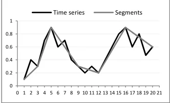
Figure 1: Sample time series segmentation.

Three basic approaches are distinct for time series segmentation: sliding windows, top–down, and bottom–up approaches. Figure 1 illustrates an example of a segmentation approach using PLA representation to the approximation of a time series

T, with length n = 20 and consecutive segments m = 6, where m is much smaller than n. The results of the segmentation approach, which aims to find the border approximation of the high-dimensional time series without losing the basic features, indicate that the time series is usually noisy and contains a large number of data points. PLA contributes to increased efficiency of the transmission, computation, and storage of the data; thus, PLA may be used to support clustering, classification, and association rule mining of time series data [2].

In the sliding window segmentation, slice implants bypass specific error thresholds. SWA has shown poor performance when applied in actual settings that involve many datasets [45]. The approach from the second top–down algorithm in the division consists of a frequent time series to achieve a standard stop [46]. This approach has the time complexity of O(n2), which excelled qualitatively from the second bottom-up algorithm [21]. In this approach, integrated segments provide the best approximation. In [47], current fast greedy algorithms improve the curriculum, and a statistical method is used to select the number of segments.

0 0.2 0.4 0.6 0.8 1

0 1 2 3 4 5 6 7 8 9 10 11 12 13 14 15 16 17 18 19 20 21

(4)

325 These segmentation methods attempt to segment a time period series, and they may be distinguished into online and offline approaches. In the online approach, an error threshold is specified by the user (experts), while the offline approach uses a dynamic error threshold that changes in accordance with specific criteria when the algorithm is executed.

2.2 Sliding Window Algorithm (SWA)

SWA is popular in various time series applications such as in the medical, weather, and financial domains. SWA is a temporal approximation over the actual value of the time series data. SWA identifies the segments of the first value of a time series and merges them to the next value until a specific error criterion is satisfied. The size of the window and segment increases until the error of the segment reaches the approximate current segment and specific threshold defined by the user. After selecting the first segment, the next segment is selected from the end of the first segment. The process is repeated until all time series data are segmented [19]. SWA obtains the

segments with lesser error than the user-specified threshold.

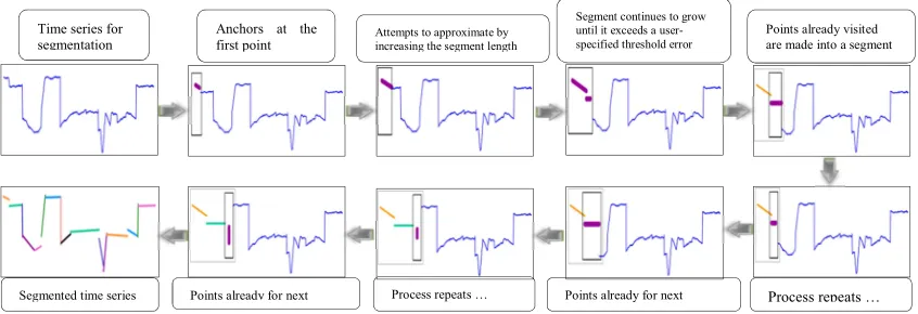
Figure 2 shows the time series segmentation based on the SWA approach, in which the time series data are split depending on a user-specific error criterion. The initial segment starts, while the first element associated with time series Tn is used.

[image:4.612.99.522.367.512.2]

This segment is grown until its cost eventually becomes higher than a predefined value. The next segment then begins at the next element. The process is repeated until the entire time series is segmented. The sliding window is simple and intuitive, but generates poor results with a few exceptions; it is a worse-performing algorithm to a large extent [2, 48]. The process described above underlines the difficulty of producing a single variant of the algorithm that is robust to arbitrary data sources, because the SWA based on PLA representation cannot divide a sequence into a predefined number of segments despite being the fastest approach [2].

Figure 2: Time series segmentation process based on the SWA approach.

The aim of SWA is to reduce the overall approximation error (e.g., Euclidean or vertical distance between the original approximation and time series) given a specific amount of information (e.g., the number of segments). These error boundaries are represented by any parameter numbers (change points) used to represent the time series, which should provide a better representation after rounding the one with the least amount of information used. Therefore, these methods do not meet our requirements and cannot be used to solve the problem.

Segmentation using SWA starts through the left border identification (anchor) from the first potential segment (usually the first data point of the time series), which is also the starting point for a window that slides (for the right point) along the

time series. Subsequently, segments that pass the predefined segmentation criterion (threshold specified by the user) can be identified and selected. In sliding down the sequence, the window size increases gradually. Considering that all data points had been visited, potential elements of the potential of the segment are instantly converted until the error of the potential segment is greater than the user-specified threshold. At this stage, the right border of the sliding window becomes known. The window size of a certain segment is then determined, and the breakpoint of the newly made segment becomes the new anchor (the starting point of any potential next segment). The algorithm and this segment generation process repeats until the entire time series has been approximated by a PLA representation. Table 1 shows the pseudo-code of Anchors at the

first point Attempts to approximate by increasing the segment length

Segment continues to grow until it exceeds a user-specified threshold error

Points already visited are made into a segment

Process repeats …

Time series for segmentation

Points already for next Process repeats …

(5)

[image:5.612.313.523.399.542.2]

326 SWA. Figure 2 illustrates the flow of the second phase of the segmentation process together with the application of SWA.

Table 1: Sliding window algorithm

With its procedural simplicity, SWA allows the growth of a segment until the error for the potential segment is in excess of the threshold specified by the user. The subsequence is then converted into a segment. The process is repeated until the entire time series is approximated by PLA representation. The first segment starts with the first element of Tn. This segment is grown until its cost exceeds a predefined value. The next segment begins at the next element. The process is repeated until the entire time series is segmented. One error estimation method involves obtaining the average of the sum of the square of the vertical differences between the best-fit line plus the actual data points. Another widely used measure with goodness of fit is the distance between the most effective fit line plus the data point furthest away in the vertical direction [2].

The change point in SWA is detected whenever the value of the time series point changes. The window size is the width of the time series points. In SWA, the width is fixed as two points in one window. The error for the change point is then computed [9]. In this paper, the original SWA is improved by incorporating the expert-specified change points for climate time series data. The adaptive SWA called ASWA uses these change points as the error criterion of the segment.

3. PROPOSED ALGORITHM

Our proposed ASWA for the weather-related time series data differs from the algorithm in our

previous work, in which we considered all identified segments across change points of weather data collected by domain experts. These change points can be used as the error criterion of the segment defined from the expert (user)-specified threshold.

ASWA is proposed to segment the time series data of rainfall and river flow. The original SWA detects errors that occur during segmentation and defines the window size as the width of two points for each detection. The important aspect of ASWA is the change point of detection and the size of the window. The change point is the change in value of the time series. In the original SWA, the change point is detected whenever the value of the time series changes. The window size is the width of the time series points, which, in SWA, is fixed as two points in one window. The error for the change point is calculated.

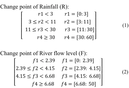
2.3 Change Point

The error for the change point in rainfall and river flow datasets is considered to account for any possibility of change in the data with respect to the classification of values. A change point represents changes that occur within four possibilities, as shown in Eq.1 for rainfall and Eq.2 for river flow:

Change point of Rainfall (R):

1 3 1 0: 3

3 2 11 2 3: 11

11 3 30 3 11: 30

4 30 4 30: 60

(1)

Change point of River flow level (F):

1 2.39 1 0: 2.39

2.39 2 4.15 2 2.39: 4.15

4.15 3 6.68 3 4.15: 6.68

4 6.68 4 6.68: 50

(2)

where R = r1,r2,r3,...,rn is a rainfall series of length

n and F = f1,f2,f3,…,fn is a river flow series of length

n. The rainfall values are classified into four different classes: No rain = [0:2] (N), Light = [3:10] (L), Moderate = [11:30] (M), and Heavy = [31:60] (H). The river flow values for Station 1 are classified into four different classes: Low = [0:2.63] (L), Medium = [2.39:4.15] (M), High = [4.15:6.68] (H), and Very High = [6.68:50] (VH). This classification is based on the trends in rainfall and river flow, which are validated by the experts of the Institute of Climate Change, University Kebangsaan Malaysia, Malaysia.

Input: a time series

1, ...,2

T=t t _tn (sequence), max_error (e)

Output: number of segmented time series

1,2...,

T =t t _{t N} (subsequence)

1 begin

2 Anchor = 1; // Starting point 3 NoSeg=1;

4 while (i < n) 5 Set i = 2

6 while (calculate_error(T[ Anchor : Anchor + i ]< max_error)

9 Set i equal to i + 1 10 end while

11 Seg_TS[NoSeg] = create_segment(T[ Anchor : Anchor + (i-1)])

12 Set Anchor = Anchor + i 13 Set NoSeg = NoSeg + 1 14 end while

(6)

327 2.4 Window Size

A sliding window moves through the time series sequences until a change point is encountered, and then the segmentation process begins. In the time series segmentation, window size (w) plays an important role in the segmented

time series subsequence. For each window or subsequence, w indicates the number of values being grouped into one window.

Table 2 illustrates a dynamic window size of segments using the proposed algorithm, ASWA. The sequence of rainfall data is from Day 1 to Day

Table 2 Sample rainfall data for 40 days

Days Windows

W1 W2 W3 W4 W5 W6 W7 W8 W9 W10

d1 0 33.4 6.1 41.5 38.1 30 34 15.4 2.8 10.9

d2 0 57 4.6 33.9 30.9 17.2 47.3 24.2 1.3 6.4 d3 0 30.1 3.6 57.9 46.3 29.7 37.5 18.9 0.3

d4 0 41.6 37.9 22.7 33.3 12.8 0.8

d5 2.6 31.9 29.5 1.5

Class N H L H H M H M N L

40. We use days for simplicity, but in actual applications, data could be at any temporal interval. In the generated segments with dynamic window size for rainfall data, the values in each window are grouped based on the proposed change point.

The rainfall database contains data collected over a period of time, and these data can be processed by a sliding window. Each window represents a sequence of timestamped data, that is, each sequence has a single timestamp. The amount of data in the window may therefore vary because the window is progressed along the time series. In distributing the rainfall data in Table 2 to the dynamic window size, 10 windows are produced.

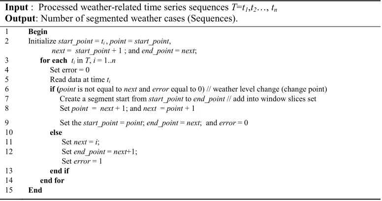
[image:6.612.113.501.492.696.2]

Table 3 presents the proposed ASWA for the segmentation of the weather-related time series data. SWA works through a time series sequence, detects change point (error) whenever the time series value changes, and then groups each two time points with the change point together as one window. Consequently, a high number of windows and low number of time points for each window are generated. Hence, we aim to improve SWA to produce the most appropriate segmentation for weather data with reduced approximation error ratio based on change point and to set the dynamic window size of obtained segments for weather-related time series data. The following are the steps in applying ASWA:

Table 3: Adapted sliding window algorithm (ASWA)

Input : Processed weather-related time series sequences T=t1,t2…, tn

Output: Number of segmented weather cases (Sequences).

1 Begin

2 Initialize start_point = ti , point = start_point, next = start_point + 1 ; and end_point = next; 3 for each ti in T, i = 1..n

4 Set error = 0 5 Read data at time ti

6 if (point is not equal to next and error equal to 0) // weather level change (change point) 7 Create a segment start from start_point to end_point // add into window slices set 8 Set point = next + 1; and next = point + 1

9 Set the start_point = point; end_point = next; and error = 0 10 else

11 Set next = i;

12 Set end_point = next+1; Set error = 1

13 end if

14 end for

(7)

328 The algorithm begins by initializing the parameters as follows: error represents the degree of change in the weather values level, start_point

represents the first point in a window at time t,

end_point represents the last point in a window, and

point represents the current time point while next

represents the next point after the current point. The weather data are read one data item at a time to detect the change point based on the change point error.

The change point error depends on the amount of weather change from one level to the next level. If the error exceeds, which marks the occurrence of a change point, then the algorithm determines the

start_point and end_point as one window. In

rainfall data, four types of change are observed, and the window width depends on the change between one point and the next point, as mentioned in Section 4.1. This step is repeated n times. In the succeeding step, the generated windows are stored in a text file in which each line represents one case (window). Each case has a different width.

4. EXPERIMENTS

Experiments were conducted with SWA enhanced to ASWA to achieve a perfect approximation based on the change point error of the weather data. The application of ASWA significantly reduces high-dimensional time series by dividing the weather sequence into appropriate, internally homogenous segments. The goal of ASWA is to extract temporal data to identify the association between non-trivial patterns in weather data, which is beneficial in detecting the patterns and event trends in the data. The performance of ASWA was evaluated by the vertical error (VE), mean square error (MSE), and compression ratio calculated using three rainfall datasets and two river flow datasets obtained from the Institute of Climate Change University Kebangsaan Malaysia, Malaysia. ASWA was compared with SWA and with the bottom–up algorithm.

2.5 Experimental Design

[image:7.612.104.506.392.497.2]

The proposed ASWA was tested on rainfall and river flow datasets from 1975 to 2009, which were collected by three stations. Table 4 shows the description of the datasets.

Table 4: Rainfall time series data characteristics

No Data Code Stations Period of record Time series length

1 Rainfall

1 16R-SK SgLui_Sel 1975–2009 12784

2 53R-Ladang Dominion 1975–2009 12784

3 8R-Empangan Sg.Semenyih 1975–2009 12784

2 River flow

4 OrgQ-SgSemenyih-KgRinching 1975–2009 12784

5 Q-SgLangat-Dengkil 1975–2009 12784

These weather-related time series data were proposed to be analyzed through segmentation. The time series segmentation approach using ASWA was implemented in the experiment to obtain meaningful patterns. ASWA can extract important patterns from large-scale time series data in terms of domains. In this context, we selected the data for rainfall and river flow because of their connection with each other and to show the usefulness of a correlation. Both rainfall and river flow data can assess the effectiveness of ASWA in segmentation and to achieve increased efficiency in monitoring time series trends in weather that shows meaningful patterns. The segmentation approach is applied for the time series analysis and for attempts to detect the most significant patterns for implementation of mining tasks, such as classification, prediction, and anomaly detection. This experiment was conducted to determine whether ASWA can maintain the

number of windows at a low error rate compared with SWA in weather data.

To compare the performances of SWA and ASWA, the number of segments and the preciseness of the approximation should be considered. This precision is measured by VE defined in Eq. 1, MSE defined in Eq. 2, and compression ratio in Eq. 3.

∑(#)*∑(#)* !"#$"̅#&'

+ (1)

,-

∑(#)*!"#$"̅#&'

(8)

329

./01 2334/5 674/!%&

+ ₉

: 100

(3)

Where 7_; is the actual time series values, 7=_< is a new value of the time series in period i represented by the average, n is the length of the time series, and N is the number of obtained segments. VE and MSE can be used to measure both the training and the validation errors. In segmentation problems, we are mainly interested in the error between the original signal and the reconstructed signal; thus, we reflect the approximation error in >7=, 7? = , … , 7A + C. In the proposed algorithm, tradeoff

parameters are present for the accuracy of the approximation and the segments number. We adjust the parameters to generate the same number of

segments in SWA and ASWA, and then compare the obtained VE, MSE, and compression ratio. 2.6 Results and Discussion

[image:8.612.94.524.299.430.2]

The result is evaluated based on four measurements: number of windows, VE, MSE, and compression ratio. The proposed ASWA is compared with SWA. Table 5 shows the results obtained by SWA and ASWA on the data from rainfall and river flow stations. The second column lists the original time points for each station. The third and seventh columns present the number of segments produced by SWA and ASWA, respectively. The error ratio is derived for both results by calculating VE and MSE.

Table 5: Number of segmented windows for SWA and ASWA

N

o Datasets

Original points

SWA ASWA

#windows

N VE MSE

Comp. Ratio (%)

#windows

N VE MSE

Comp. Ratio (%)

1

R

ai

n

fa

ll Station 1 12784 3559 0.116 0.249 28 % 4930 0.130 0.196 39 %

2 Station 2 12784 3624 0.131 0.322 28 % 4988 0.130 0.342 39 %

3 Station 3 12784 4245 0.122 0.290 33 % 6066 0.115 0.218 47 %

4

R

iv

er

fl

o

w Station 1 12784 731 0.060 0.006 6 % 1662 0.062 0.006 13 %

5 Station 2 ₁₂₇₈₄ ₁₂₁₀ _0.213 _0.578 _{9 %} ₂₆₉₀ _0.165 _0.479 _{21 %}

Average 2674 0.128 0.289 21 % 4067 0.120 0.248 32 %

The basic criterion to determine the better algorithm between SWA and ASWA is the number of windows. As discussed in [48], having a larger number of windows through segmentation is better. As shown in Table 5, ASWA has a higher average number of generated windows than SWA. ASWA generated 4067 large windows at the original time points of 12784, while SWA generated an average of 2674 windows.

The results in Table 5 also indicate that ASWA achieved better VE and MSE rates on most of the datasets than SWA. ASWA indicated lower VE in three datasets, namely, rainfall at Stations 2 and 3 and river flow at Station 2, while SWA obtained lower results in two datasets, namely, rainfall at Station 1 and river flow at Station 1. In calculating the mean of the error rates for the five datasets, a lower error rate was achieved by ASWA. ASWA has a slightly lower error rate of 0.120 than SWA at 0.128. Meanwhile, in comparing the two algorithms based on MSE, we obtain a lower error rates on four datasets, namely, rainfall at Stations 1 and 3 and river flow at Stations 1 and. SWA obtained lower results only in one dataset (rainfall at Station 2). Therefore, the average of MSE for the five datasets is achieved by

[image:8.612.314.520.506.611.2]

ASWA at a lower error rate of 0.248 compared with SWA at 0.289. In addition, the compression ratio of the five datasets is superior for the entire weather data that were used, with an average of 32%.

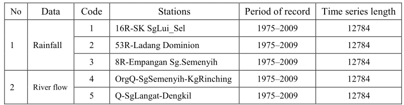
Figure 3 Number of windows generated by SWA and ASWA in five stations.

Figure 3 shows that ASWA generated more windows in all weather stations, which means that ASWA could include more time series points in a window because of the enhancement of the change point error. The enhancement of change points in

0 2000 4000 6000 8000 10000 12000 14000

Orginal points

(9)

[image:9.612.92.525.57.233.2]

330

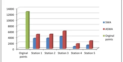
Figure 4: Approximation errors obtained by SWA and ASWA: vertical error (a), mean square error (b), and compression ratio (c).

ASWA results in each extracted window having an almost equal distribution of values and all windows having dynamic window size; by contrast, SWA extracts windows based on the linear square error that occurs as a change point during the process while the window size remains at the dynamic size [49]. As shown in Figure 3, the number of extracted windows depends on the data size. For example, Station 2 has 12784 time points that are then transferred into 4988 windows by ASWA; SWA transferred these time points into 3624 windows only.

The performance of SWA and ASWA are based on three criteria, namely, VE, MSE, and compression ratio (%). Figure 4 shows the results of the approximation errors obtained by ASWA and SWA in the five weather stations. The following are observed: A lower VE ratio is achieved by ASWA in three stations, while a lower MSE ratio is achieved in four stations. For the compression ratio, ASWA produced high compression ratios in all stations.

The results of our experiments and analyses showed that the proposed ASWA can potentially generate lower error rates and higher compression ratio of weather data than SWA. The adaptive behavior of ASWA is experimentally proven to achieve better performance by splitting the length of a time series. In essence, using the change points of weather segmentation with ASWA can reduce the data from n dimensions to N dimensions by splitting the time series into N arbitrary length segments. The algorithm can also identify meaningful patterns with different lengths throughout a time series. These patterns will not be disregarded if they are observed across time (cutting) points. Therefore, in this study, ASWA is shown to improve the segmentation of weather-related time series data in terms of its change points.

5. CONCLUSION

Segmentation approach is an important concern in time series analysis. In segmentation, a number of algorithms with different partitioning methods have attempted to reduce high-dimensional data or extract meaningful patterns from the time series sequence. SWA is one of such time series segmentation approaches that are used to reduce a large amount of time series data based on a user-specified error criterion. The proposed method called ASWA aims to improve the segmentation performed by SWA using change points of weather data as error criteria. The experiment involved 35 years of rainfall and river flow data collected from UKM’s Climate Change Institute. The results verified the ability of ASWA in finding appropriate segments of time series by extracting high information that refers to large windows with less error compared with that of SWA in some weather data. The quantitative results indicate that ASWA performs better than SWA on the number of windows, VE, MSE, and compression ratio. The findings of this study are beneficial when analyzing time series data, in which windows from time series may generate meaningful information that would otherwise be lost during the implementation of less efficient methods.

(10)

331 ACKNOWLEDGEMENTS.

This work is supported by National University of Malaysia (UKM), Research Project, Grant No. AP-2013-007, UKM.

REFRENCES:

[1] S.-y. Jiang, et al., "Approximate equal frequency discretization method," in

Intelligent Systems, 2009. GCIS'09. WRI

Global Congress on, 2009, pp. 514-518.

[2] E. Keogh, et al., "Segmenting time series: A survey and novel approach," Data mining in

time series databases, vol. 57, pp. 1-22, 2004.

[3] P. Patel, et al., "Mining motifs in massive time series databases," in Data Mining, 2002. ICDM 2003. Proceedings. 2002 IEEE

International Conference on, 2002, pp.

370-377.

[4] G. Das, et al., "Rule Discovery from Time Series," in KDD, 1998, pp. 16-22.

[5] T.-c. Fu, et al., "Financial Time Series Segmentation based on Specialized Binary Tree Representation," in DMIN, 2006, pp. 3-9.

[6] J. Jiang, et al., "A new segmentation algorithm to stock time series based on PIP approach," in Wireless Communications, Networking and Mobile Computing, 2007.

WiCom 2007. International Conference on,

2007, pp. 5609-5612.

[7] V. Guralnik and J. Srivastava, "Event detection from time series data," in

Proceedings of the fifth ACM SIGKDD

international conference on Knowledge

discovery and data mining, 1999, pp. 33-42.

[8] J. J. Oliver, et al., "Minimum message length segmentation," in Research and Development

in Knowledge Discovery and Data Mining,

ed: Springer, 1998, pp. 222-233.

[9] L. J. Fitzgibbon, et al., "Change-point estimation using new minimum message length approximations," in PRICAI 2002:

Trends in Artificial Intelligence, ed: Springer,

2002, pp. 244-254.

[10] C. L. Fancourt and J. C. Principe, "Competitive principal component analysis for locally stationary time series," Signal

Processing, IEEE Transactions on, vol. 46,

pp. 3068-3081, 1998.

[11] J. Abonyi, et al., "Fuzzy clustering based segmentation of time-series," in Advances in

Intelligent Data Analysis V, ed: Springer,

2003, pp. 275-285.

[12] Z. J. Wang and P. Willett, "Joint segmentation and classification of time series using class-specific features," Systems, Man, and Cybernetics, Part B: Cybernetics, IEEE

Transactions on, vol. 34, pp. 1056-1067,

2004.

[13] V. Megalooikonomou, et al., "A multiresolution symbolic representation of time series," in Data Engineering, 2005. ICDE 2005. Proceedings. 21st International

Conference on, 2005, pp. 668-679.

[14] F.-L. Chung, et al., "Flexible time series pattern matching based on perceptually important points," in International Joint

Conference on Artificial Intelligence

Workshop on Learning from Temporal and

Spatial Data, 2001, pp. 1-7.

[15] J. Yin, et al., "Financial time series segmentation based on Turning Points," in

System Science and Engineering (ICSSE),

2011 International Conference on, 2011, pp.

394-399.

[16] H. Azami, et al., "Automatic signal segmentation using the fractal dimension and weighted moving average filter," Journal of

Electrical & Computer science, vol. 11, pp.

8-15, 2011.

[17] E. Bingham, et al., "Segmentation and dimensionality reduction," in SDM, 2006, pp. 372-383.

[18] E. Terzi and P. Tsaparas, "Efficient Algorithms for Sequence Segmentation," in

SDM, 2006, pp. 316-327.

[19] T. Palpanas, et al., "Online amnesic approximation of streaming time series," in

Data Engineering, 2004. Proceedings. 20th

339-349.

[20] D. Lemire, "A Better Alternative to Piecewise Linear Time Series Segmentation," in SDM, 2007, pp. 545-550.

[21] J. Hunter and N. McIntosh, "Knowledge-based event detection in complex time series data," in Artificial Intelligence in Medicine, ed: Springer, 1999, pp. 271-280.

[22] M. Brooks, et al., "Scale-based monotonicity analysis in qualitative modelling with flat segments," 2005.

[23] M. Sharifzadeh, et al., "Change detection in time series data using wavelet footprints," in

Advances in Spatial and Temporal Databases,

ed: Springer, 2005, pp. 127-144.

(11)

332

Knowledge-Based Systems, vol. 23, pp.

316-322, 2010.

[25] X. Huang, et al., "Hinging hyperplanes for time-series segmentation," Neural Networks and Learning Systems, IEEE Transactions on,

vol. 24, pp. 1279-1291, 2013.

[26] J. Abonyi, et al., "Modified Gath–Geva clustering for fuzzy segmentation of multivariate time-series," Fuzzy Sets and

Systems, vol. 149, pp. 39-56, 2005.

[27] J. H. Chang and W. S. Lee, "Finding recent frequent itemsets adaptively over online data streams," in Proceedings of the ninth ACM

SIGKDD international conference on

Knowledge discovery and data mining, 2003,

pp. 487-492.

[28] H.-F. Li and S.-Y. Lee, "Mining frequent itemsets over data streams using efficient window sliding techniques," Expert Systems

with Applications, vol. 36, pp. 1466-1477,

2009.

[29] H. Chen, "Mining top-k frequent patterns over data streams sliding window," Journal of

Intelligent Information Systems, vol. 42, pp.

111-131, 2014.

[30] F. Nori, et al., "A sliding window based algorithm for frequent closed itemset mining over data streams," Journal of Systems and

Software, vol. 86, pp. 615-623, 2013.

[31] G. Lee, et al., "Sliding window based weighted maximal frequent pattern mining over data streams," Expert Systems with

Applications, vol. 41, pp. 694-708, 2014.

[32] T.-P. Chang, "A Sliding-Window Method to Discover Recent Frequent Query Patterns from XML Query Streams," International

Journal of Software Engineering and

Knowledge Engineering, vol. 24, pp. 955-980,

2014.

[33] K. Xu, et al., "PRESEE: An MDL/MML

Algorithm to Time-Series Stream

Segmenting," The Scientific World Journal,

vol. 2013, 2013.

[34] X. Liu, et al., "Novel online methods for time series segmentation," Knowledge and Data

Engineering, IEEE Transactions on, vol. 20,

pp. 1616-1626, 2008.

[35] E. Fuchs, et al., "Online segmentation of time series based on polynomial least-squares approximations," Pattern Analysis and Machine Intelligence, IEEE Transactions on,

vol. 32, pp. 2232-2245, 2010.

[36] L. A. Romani, et al., "A new time series mining approach applied to multitemporal remote sensing imagery," Geoscience and

Remote Sensing, IEEE Transactions on, vol.

51, pp. 140-150, 2013.

[37] V. Dakos, et al., "Slowing down as an early warning signal for abrupt climate change,"

Proceedings of the National Academy of

Sciences, vol. 105, pp. 14308-14312, 2008.

[38] H. Von Storch, et al., "Relationship between global mean sea-level and global mean temperature in a climate simulation of the past millennium," Ocean Dynamics, vol. 58, pp. 227-236, 2008.

[39] H. von Storch, et al., "Assessment of three temperature reconstruction methods in the virtual reality of a climate simulation,"

International Journal of Earth Sciences, vol.

98, pp. 67-82, 2009.

[40] S. A. Nunes, et al., "Analysis of large scale climate data: how well climate change models and data from real sensor networks agree?," in

Proceedings of the 22nd international

conference on World Wide Web companion,

2013, pp. 517-526.

[41] S. A. Nunes, et al., "To be or not to be real: fractal analysis of data streams from a regional climate change model," in

Proceedings of the 27th Annual ACM

Symposium on Applied Computing, 2012, pp.

831-832.

[42] E. J. Keogh and M. J. Pazzani, "An Enhanced Representation of Time Series Which Allows Fast and Accurate Classification, Clustering and Relevance Feedback," in KDD, 1998, pp. 239-243.

[43] Q. Chen, et al., "Indexable PLA for efficient similarity search," in Proceedings of the 33rd international conference on Very large data

bases, 2007, pp. 435-446.

[44] H. Shatkay and S. B. Zdonik, "Approximate queries and representations for large data sequences," in Data Engineering, 1996. Proceedings of the Twelfth International

Conference on, 1996, pp. 536-545.

[45] J. Lin, et al., "A symbolic representation of time series, with implications for streaming algorithms," in Proceedings of the 8th ACM SIGMOD workshop on Research issues in

data mining and knowledge discovery, 2003,

pp. 2-11.

[46] S.-H. Park, et al., "Representation and clustering of time series by means of segmentation based on PIPs detection," in

Computer and Automation Engineering

(ICCAE), 2010 The 2nd International

(12)

333 [47] J. Himberg, et al., "Time series segmentation

for context recognition in mobile devices," in

Data Mining, 2001. ICDM 2001, Proceedings

IEEE International Conference on, 2001, pp.

203-210.

[48] E. Keogh, et al., "An online algorithm for segmenting time series," in Data Mining, 2001. ICDM 2001, Proceedings IEEE