A NEW SOFT SET BASED PRUNING ALGORITHM FOR ENSEMBLE METHOD

(1)

ISSN: 1992-8645 www.jatit.org E-ISSN: 1817-3195

A NEW SOFT SET BASED PRUNING ALGORITHM FOR

ENSEMBLE METHOD

*

1MOHDKHALID AWANG, 1MOKHAIRI MAKHTAR, 1M NORDIN A RAHMAN, 2MUSTAFA

MAT DERIS

1

Faculty of Informatics and Computing, Universiti Sultan Zainal Abidin,

22000 Tembila, Terengganu, Malaysia 2

Faculty of Computer Science and Information Technology,

Universiti Tun Hussein Onn Malaysia (UTHM)

Batu Pahat, Johor, Malaysia

*Corresponding author: [email protected]

ABSTRACT

Ensemble methods have been introduced as a useful and effective solution to improve the performance of the classification. Despite having the ability of producing the highest classification accuracy, ensemble methods have suffered significantly from their large volume of base classifiers. Nevertheless, we could overcome this problem by pruning some of the classifiers in the ensemble repository. However, only a few researches focused on the ensemble pruning algorithm. Therefore, this paper aims to increase classification accuracy and at the same time minimizing ensemble classifiers by constructing a new ensemble pruning method (SSPM) based on dimensionality reduction in soft set theory. Ensemble pruning deals with the reduction of predictive models in order to improve its efficiency and predictive performance. Soft set theory has been proved to be an effective mathematical tool for dimension reduction. Thus, we proposed a novel soft set based method to prune the classifiers from heterogeneous ensemble committee and select the best subsets of the component classifiers prior to the combination process. The results show that the proposed method not only reduce the number of members of the ensemble, but able to produce highest prediction accuracy.

Keywords: Ensemble Pruning, Ensemble Selection, Soft Set, Ensemble Methods

1. INTRODUCTION

Ensemble methods or multiple classifiers are known as learning algorithms that train a set of classifiers and combine them to achieve the best prediction accuracy [1]. Previous works have shown that combining the predictions of a collection of classifiers can be an effective strategy to improve generalization performance, such as bagging [2], boosting [3], stacking [4], Bayes optimal classifier [5], rotation forest [5], ensemble selection [6] and hybrid intelligent system [7].

The most fundamental concepts of ensemble methods consist of two main stages which is the production of multiple base classifier models and their combination. One of the noticeable disadvantages of ensemble methods is the production of a large number of individuals which sometimes referred as overproduce. Recent work

[8,9] considered an additional intermediate phase that deals with the reduction of the ensemble size prior to the combination. This phase is known as ensemble pruning, selective ensemble or ensemble thinning [8-12]. Regardless of the name, ensemble pruning deals with the reduction of predictive models in order to improve its efficiency and predictive performance. Ensemble pruning focuses on finding the minimal number of base classifiers from a repository of classifiers and at the same time maining the classification or prediction performance. However, despite of the importance of the pruning phase, only a few researches focused on the selection of ensemble’s classifiers.

(2)

ISSN: 1992-8645 www.jatit.org E-ISSN: 1817-3195 based on the dimensionality reduction of soft set

theory.

The rest of this paper is organized as follows. Section 2 describes the ensemble methods and ensemble pruning. Section 3 discusses the soft set and its reduction algorithm. Section 4, soft set pruning method (SSPM) describes the soft set theoretical analysis of the granular metadata generated by the decisions of base classifiers. Section 5 describes the experimental setting and results. Finally, Section 6 summarizes this work.

2. ENSEMBLE METHODS AND ENSEMBLE

PRUNING

Previous researchers have proposed various ensemble methods as learning algorithms in data mining to improve the classifiers performance and accuracy. There is no single ensemble methods that dominate classification technique. Most of the previous studies focus on the ensemble construction and ensemble combination in improving the accuracy and performance of classification, but rarely consider the ensemble pruning algorithms. Nevertheless, there are few researches focusing on ensemble pruning methods [8-13].

Previous ensemble pruning techniques can be categorized into three branches, the ordering-based pruning, the clustering-based pruning and the optimization-based pruning. Tsoumakas et al. [2009] provided a brief taxonomy on ensemble pruning. Order-Based Pruning ranks the individual classifiers according to some criterion. The classifiers in the front-part of the rank will be considered as the best candidate to form the final ensemble. Reduce-Error Pruning [14], Kappa Pruning [15] and Boosting-Based Pruning [16] are belongs category. On the hand, the Clustering-Based Pruning identifies a number of representatives of individual classifiers to construct the final ensemble. Ensemble pruning groups together the individual classifiers into a number of clusters based on their similarities. Some of the works in this method including Hierarchical Agglomerative Clustering [17], k-means Clustering [18] and Deterministic Annealing [19]. The last category is the Optimization-Based Pruning, which aims to select the subset of individual classifiers that maximizes or minimizes an objective related to the final ensemble. Some researchers under this category proposed Mathematical Programming Pruning [20] and Probabilistic Pruning [21].

3. SOFT SET THEORY

Soft set is a parametrized general mathematical tool which deals with a collection of approximate descriptions of objects. Each approximate description has two parts, a predicate and an approximate value set. In classical mathematics, a mathematical model of an object is constructed and define the notion of the exact solution of this model. Usually the mathematical model is too complicated and the exact solution is not easily obtained. So, the notion of approximate solution is introduced and the solution is calculated. In the soft set theory, we have the opposite approach to this problem. The initial description of the object has an approximate nature, and we do not need to introduce the notion of exact solutions. The absence of any restrictions on the approximate description of soft set theory makes this theory very convenient and easily applicable in practice. Any parameterization we prefer can be used with the help of words and sentences, real numbers, functions, mappings and so on.

Soft set theory has potential applications in many different fields which include the smoothness of functions, game theory, operations research, Riemann integration, Perron integration, probability theory, and measurement theory, attribute and feature reduction [22-25]

a) Basic Concept of Soft Set

Let U be initial universal set and let E be a set of parameters. Let P(U) denote the power set of U. A pair (F, E) is called a soft set over U, if only if F is a mapping given by F:E P(U) [22,23].

b) Soft Set Reduction based on Discernibility Function

The most fundamental concept in rough set is set approximation and it is carried out by indiscernibility function. Based on [24] that every rough set is a soft set, we proposed a similar concept of discernibility function in rough set [25,26] to reduct and discern the soft set data.

4. PROPOSED SOFT SET PRUNING

ENSEMBLE METHOD (SSPM)

(3)

ISSN: 1992-8645 www.jatit.org E-ISSN: 1817-3195 classifiers. The process of reducing the number of

classifiers is known as pruning. The first step in the soft set pruning ensemble methods is to generate the decision table of the testing data set. The decision table is then transformed into a soft set representation. The next step is to apply the reduction algorithm on the soft set table. Based on [24] that every rough set is a soft set, we proposed a a similar concept of discernibility function in rough set [25] to reduct and discern the data sets. Then the table will be transformed into discernibility matrix. The next step is to perform the discernibility function on the discernibility matrix. The discernibility function will produce set of reducts. Finally, we apply the distributive law on the reduct to generate reduct teams.

A New Soft Set Ensemble Pruning Algorithm

Input: Decision tables of the testing dataset Output: Team/teams of ensemble

1. Start

2. Construct the decision table of

the testing data set.

3. Transform the decision table

into softest representation

4. Transform the softest

representation into

discernibility matrix

5. Transform the discernibility

matrix into discernibility

function

6. Apply the absorption law to get

the set of the reduct.

7. Apply the distributive law to

construct the reduct teams

8. End

A. Soft Ensemble Representation

Suppose that there are M _instances_{in the test data}

set which consist of (r1, r2, r3, r4, r5, r6, r7) and N number of classifiers in our pool of classifiers such as (c1, c2, c3, c4). Each instance of test data set is mapped against each type of classifiers to produce

N numbers of prediction output.

Step 2: The M X N matrix is considered as the

decision table representing the M numbers of instances and N number of classifiers.

Table 1: An Example of Prediction Output

U _c₁ _c₂ _c₃ _c₄

r1 yes no yes no

r2 yes yes no no

r3 yes yes yes yes

r4 no yes no yes

r5 no no yes no

r6 no no no no

r7 no no yes no

A Prediction Output is defined as a 7-tuple S = (U, A, V, f), where

U

=

{

u

₀

,

u

₁

,

L

,

u

_U₋₁

,

u

_U

}

is a

non-empty finite set of objects,

{

a

A

a

A

}

A

=

₀

,

₁

,

L

,

₋₁

,

is a non-empty finite

set of attributes,

U

A e

e

i i

V

∈

=

, where

V

_a

is the domain (value set) of attribute a ,

V

A

U

f

:

×

→

is an information

(

x

a

)

V

a

f

,

∈

Function, such that, for ever

f

(

x

,

a

)

∈

V

_a .

Definition 1. (Molodtsov, 1999) Let U be initial

universal set and let E be a set of parameters. Let

P(U) denote the power set of U. A pair (F, E) is called a soft set over U, if only if F is a mapping given by F:E P(U).

Suppose that there are seven (7) instances in the dataset under consideration

U= {r1,r2,r3,r4,r5,r6,r7}

and E is a set of parameter representing ensemble of classifiers

E= {c1,c2,c3,c4} Where

c1 stands for “classifier1” c2 stands for “classifier2” c3 stands for “classifier3” c4 stands for “classifier4”

Suppose that

F(c1)={r1,r2,r3},

F(c2)={r2,r3,r4},

F(c3)={r1,r3,r5,r7},

F(c4)={r3,r4},

we can view the soft set (F, E) as a collection of

classifier1={r1,r2,r3},

classifier2={r2,r3,r4},

classifier3={r1,r3,r5,r7},

(4)

ISSN: 1992-8645 www.jatit.org E-ISSN: 1817-3195 Consider the mapping F:E

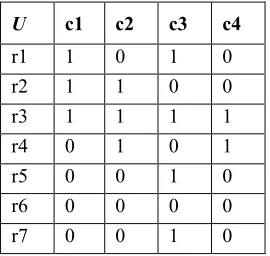
Step 3: Thus, we can make one-to-one

corresponding between a Boolean-valued prediction results and a soft set, as stated in

[image:4.612.128.263.193.321.2]

proposition 1

Table 2 : Boolean-Valued of Classifier’s Prediction

U _c1 _c2 _c3 _c4

r1 1 0 1 0

r2 1 1 0 0

r3 1 1 1 1

r4 0 1 0 1

r5 0 0 1 0

r6 0 0 0 0

r7 0 0 1 0

Proposition 1. If (F, E) is a soft set over the

universe U, then (F, E) is a Boolean-valued information system S = (U,A,V{0,1} , f).

Step 4: For the information system S from Table 2

we obtain the discernibility matrix presented in Table 3, and the following discernibility functions:

Table 3 : Boolean-Valued of Classifier’s Prediction

r1 r2 r3 r4 r

5 r 6

r 7 r

1

0

r 2

c2,c3 0

r

3

c2,c4 c3,c4 0

r

4

c1,c2,c3, c4

c1,c4 c1,c3 0

r

5

c1 c1,c2,c

3

c1,c2,c4 c2,c3, c4

0

r 6

c1,c3 c1,c2 c1,c2,c3, c4

c2,c4 c 3

0

r 7

c1 c1,c2,c 3

c1,c2,c4 c2,c3, c4

0 c 3

0

Step 5 : The discernibility functions are as follows:

f(r1)={c2ѵc3}ʌ{c2ѵc4}ʌ{c1ѵc2ѵc3ѵc4}ʌ {c1}ʌ{c1ѵc3}ʌ{c1};

f(r2)={c3ѵc4}ʌ{c1ѵc4}ʌ{c1ѵc2ѵc3}ʌ{c1 ѵc2}ʌ{c1ѵc2ѵc3};

f(r3)={c1ѵc3}ʌ{c1ѵc2ѵc4}ʌ{c1ѵc2ѵc3ѵ c4}ʌ{c1ѵc2ѵc4};

f(r4)={c2ѵc3ѵc4}ʌ{c2ѵc4}ʌ{c2ѵc3ѵc4}; f(r5)={c3};

f(r6)={c3};

Step 6: Generating the reduct based on the

following indiscernibility functions:

f(ri) = f(r1) ʌ f(r2) f(r3) ʌ f(r4) ʌ f(r5) ʌ f(r6) ʌ f(r7)

f(R) = EmptySet;

by applying the absorption law for each f(ri), we obtain the following:

[step 6.1]

f(r1)={c2ѵc3}ʌ{c2ѵc4}ʌ{c1ѵc2ѵc3 ѵc4}ʌ{c1}ʌ{c1ѵc3}ʌ{c1}

f(R)=f(R)ʌf(r1)

f(R) = {}

f(R1)= {}ʌ {c2ѵc3};

f(R)={c2ѵc3}

f(R)={c2ѵc3}ʌ{c2ѵc4};

f(R)={c2ѵc3}ʌ{c2ѵc4}

f(R)={c2ѵc3}ʌ{c2ѵc4}ʌ{c1ѵc2ѵc3ѵ c4};

f(R)={c2ѵc3}ʌ{c2ѵc4}

f(R)={c2ѵc3}ʌ{c2ѵc4}ʌ{c1};

f(R)={c2ѵc3}ʌ{c2ѵc4}ʌ{c1}

f(R)={c2ѵc3}ʌ{c2ѵc4}ʌ{c1}ʌ{c1ѵc 3};

f(R)={c2ѵc3}ʌ{c2ѵc4}ʌ{c1}

f(R)={c2ѵc3}ʌ{c2ѵc4}ʌ{c1}ʌ{c};

f(R)={c2ѵc3}ʌ{c2ѵc4}ʌ{c1}

f(R)= {c2ѵc3}ʌ{c2ѵc4}ʌ{c1}

[step 6.2]

f(r2)=

{c3ѵc4}ʌ{c1ѵc4}ʌ{c1ѵc2ѵc3}ʌ{c1ѵ c2}ʌ{c1ѵc2ѵc3}

f(R)=f(R)ʌf(r2)

f(R)ʌf(R2)={c2ѵc3}ʌ{c2ѵc4}ʌ{c1}ʌ

{c3ѵc4};

f(R)=

(5)

ISSN: 1992-8645 www.jatit.org E-ISSN: 1817-3195 f(R)={c2ѵc3}ʌ{c2ѵc4}ʌ{c1}ʌ{c3ѵc

4}ʌ{c1ѵc4};

f(R)={c2ѵc3}ʌ{c2ѵc4}ʌ{c1}ʌ{c3ѵc 4}

f(R)={c2ѵc3}ʌ{c2ѵc4}ʌ{c1}ʌ{c3ѵc 4}ʌ{c1ѵc2ѵc3};

f(R)={c2ѵc3}ʌ{c2ѵc4}ʌ{c1}ʌ{c3ѵc 4}ʌ{c1ѵc2};

f(R)={c2ѵc3}ʌ{c2ѵc4}ʌ{c1}ʌ{c3ѵc 4}ʌ{c1ѵc2ѵc3};

f(R)=

{c2ѵc3}ʌ{c2ѵc4}ʌ{c1}ʌ{c3ѵc4}

[step6.3]

f(r3)={c1ѵc3}ʌ{c1ѵc2ѵc4}ʌ{c1ѵc2 ѵc3ѵc4}ʌ{c1ѵc2ѵc4}

f(R)=f(R)ʌf(r3)

f(R)=

c2ѵc3}ʌ{c2ѵc4}ʌ{c1}ʌ{c3ѵc4}ʌ{c1 ѵc3};

f(R)=

f(R)=c2ѵc3}ʌ{c2ѵc4}ʌ{c1}ʌ{c3ѵc4 }ʌ{c1ѵc2ѵc4}

f(R)=

f(R)=c2ѵc3}ʌ{c2ѵc4}ʌ{c1}ʌ{c3ѵc4 }ʌ{ c1ѵc2ѵc3ѵc4}

f(R)=

f(R)=c2ѵc3}ʌ{c2ѵc4}ʌ{c1}ʌ{c3ѵc4 }ʌ{ c1ѵc2ѵc4}

f(R)=

[step 6.4]

f(r4)={c2ѵc3ѵc4}ʌ{c2ѵc4}ʌ{c2ѵc3 ѵc4}

f(R)=f(R)ʌf(r4)

f(R)=

{c2ѵc3}ʌ{c2ѵc4}ʌ{c1}ʌ{c3ѵc4}ʌ{ c2ѵc3ѵc4};

f(R)=

f(R)=c2ѵc3}ʌ{c2ѵc4}ʌ{c1}ʌ{c3ѵc4 }ʌ{c2ѵc4}

f(R)=

[step 6.5]

f(r5)={c3}

f(R)=f(R)ʌf(r5)

f(R)=

{c2ѵc3}ʌ{c2ѵc4}ʌ{c1}ʌ{c3ѵc4}ʌ{ c3};

f(R)= {c2ѵc4}ʌ{c1}ʌ{c3}

[step 6.6]

f(r6)={c3}

f(R)=f(R)ʌf(r6)

f(R)=

{c2ѵc3}ʌ{c2ѵc4}ʌ{c1}ʌ{c3ѵc4}ʌ{ c3};

f(R)= {c2ѵc4}ʌ{c1}ʌ{c3}

Step 7: At the end of the discernibility function, we

applied the distributive law to gain the final reducts. By applying the distributive law for each of f(R), we obtain the following:

f(R)= {c2ѵc4}ʌ{c1}ʌ{c3}

R1 = {c2,c1,c3}

(6)

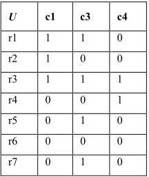
ISSN: 1992-8645 www.jatit.org E-ISSN: 1817-3195 The following tables represent the output of the

[image:6.612.141.250.178.309.2]

reducts generation. In this example, the proposed soft set pruning algorithm produces 2 different teams of ensembles.

Table 4 : Boolean-Valued of Classifier’s Predicted Reduction R1

U _c1 _c2 _c3

r1 1 0 1

r2 1 1 0

r3 1 1 1

r4 0 1 0

r5 0 0 1

r6 0 0 0

r7 0 0 1

Table 5 : Boolean-Valued of Classifier’s Prediction Reduction R2

U c1 c3 c4

r1 1 1 0

r2 1 0 0

r3 1 1 1

r4 0 0 1

r5 0 1 0

r6 0 0 0

r7 0 1 0

Based on the reduction method, we can reduce the ensemble size and select the team to produce a good and efficient ensemble.

5. EXPERIMENTAL EVALUATION

In order to validate the performance of the proposed soft set ensemble pruning algorithm, we construct our ensemble on breast cancer datasets from the UCI machine learning data repository [27]. We create our heterogeneous ensemble by selecting ten different classifiers which are listed in Table 6.

Table 6 : Classifier Prediction

Classifiers Team

Representation

Prediction Accuracy weka.classifiers.meta.EnsembleSelection 0000000001 0.72 weka.classifiers.rules.DecisionTable 0000000010 0.74 weka.classifiers.meta.StackingC 0000000100 0.75 weka.classifiers.meta.AdaBoostM1 0000001000 0.74 weka.classifiers.meta.Bagging 0000010000 0.74 weka.classifiers.rules.ZeroR 0000100000 0.75 weka.classifiers.bayes.NaiveBayesUpdatea

ble

0001000000 0.74

weka.classifiers.rules.JRip 0010000000 0.79 weka.classifiers.trees.J48 0100000000 0.77 weka.classifiers.lazy.IBk 1000000000 0.74

[image:6.612.141.249.349.477.2]

Table 6 displays the prediction accuracy of each of the classifiers with the highest accuracy of an individual classifier is 0.79%. Based on the number of classifiers in the ensemble, we could end up with 1653 combination of different classifiers team as illustrated in Table 7.

Table 7 : Number of Classifier Before and After Pruning

Original Ensemble

After Soft set Pruning Number of classifiers

in original ensemble

10 8

Number of all possible

combinations of classifiers

1653 1024

Table 7 shows the size of ensemble before and after the soft set pruning algorithm. The original set of ensemble consist 10 classifiers which is:

{

c1,c2,c3,c4,c5,c6,c7,c8,c9,c10}.

The soft set pruning algorithms take out {c5,c8} and produce the a new subset which is:

{c1,c2,c3,c4,c6,c7,c9,c10}.

[image:6.612.328.509.351.449.2]

(7)

ISSN: 1992-8645 www.jatit.org E-ISSN: 1817-3195 Table 8 : Ensemble Combination with the Highest

Accuracy

Ensemble of Classifiers

FULL ensemble

or Pruned

Prediction Accuracy

Number of Classifiers in

Ensemble

1011011110 Full 0.81 7

0111011110 Full 0.81 7

0011101010 Full 0.81 5

0011001110 Full 0.81 5

1011011010 Pruned 0.81 6 0111011010 Pruned 0.81 6

1010011010 Pruned 0.81 5 1010011010 Pruned 0.81 5 0111010010 Pruned 0.81 5 0110011010 Pruned 0.81 5

0011001010 Pruned 0.81 4

0011000010 Pruned 0.81 3

0010001010 Pruned 0.81 3

Table 8 shows that all possible combinations of classifiers in the ensemble methods that produce the best prediction accuracy. It’s apparent that the performance of the ensemble classifiers is better than single classifiers. Furthermore, the ensembles also contain the minimum number of classifiers based on soft set reduction. The experimental result shows that the performance of the proposed soft set based pruning is as good as the full ensemble. The number of classifiers in the pruned ensembles varies from 3 which is the minimum and up to 6, which is the maximum. The total number of original data sets is 8. This is an obvious improvement over full ensemble. The best ensemble could be either 0011000010 =

{c3,c4,c9} or 0010001010

={c3,c7,c9}.

6. CONCLUSION

In this paper, a new soft set based ensemble pruning method is proposed. Heterogeneous ensemble is generated based on ten different classifier algorithms. It’s acknowledged that the most significant advantage of soft set theory is its great ability of dimensionality reduction. Based on this soft set reduction algorithm, the ensemble is pruned and only a subset of the classifiers is considered prior to ensemble combination. From the experiments, we could claim that soft set ensemble pruning algorithm is able to produce the highest prediction accuracy with the minimum number of classifiers. Nevertheless, there could be several directions to

explore in the future works. One of our future works will be on discovering an algorithm for ensemble combination based on soft set theory.

ACKNOWLEDGEMENT

This work is partially supported by UniSZA (Grant No. UniSZA/14/GU/(022) and KPT(Grant No. FRGS/2/2013/ICT07/UniSZA/02/2).

REFRENCES:

[1] Dietterich, T. G. ,“Ensemble methods in machine learning. In Multiple classifier systems, Springer Berlin Heidelberg, 2000,

pp. 1-15

[2] Breiman, L. , “Bagging predictors. Machine learning,” 24(2), 1996, pp. 123-140

[3] Freund, Y., & Schapire, R. E., Experiments with a new boosting algorithm,” In ICML, 1996, July, (Vol. 96, pp. 148-156)

[4] Breiman, L., “Stacked regressions. Machine learning”, 24(1), 1996, pp. 49-64

[5] Wang, H., Fan, W., Yu, P. S., & Han, J. , “ Mining concept-drifting data streams using ensemble classifiers.” In Proceedings of the ninth ACM SIGKDD international conference on Knowledge discovery and data mining, ACM, August,2003, pp.226-235

[6] Rodriguez, J. J., Kuncheva, L. I., & Alonso, C. J. , “Rotation forest: A new classifier ensemble method. Pattern Analysis and Machine Intelligence,” IEEE Transactions on, 28(10), 2006, pp.1619-1630.

[7] Caruana, R., Niculescu-Mizil, A., Crew, G., & Ksikes, A “Ensemble selection from libraries of models,” In Proceedings of the twenty-first international conference on Machine learning

ACM, July 2004, pp 18

[8] Tsoumakas, G., Partalas, I., & Vlahavas, I. , “ A taxonomy and short review of ensemble selection,” In Workshop on Supervised and Unsupervised Ensemble Methods and Their Applications, July 2008.

[9] Partalas, I., Tsoumakas, G., Katakis, I., & Vlahavas, I. “Ensemble pruning using reinforcement learning,” In Advances in Artificial Intelligence Springer Berlin Heidelberg. 2006, pp.301-310

[10]Martinez-Muoz, G., Hernández-Lobato, D., & Suarez, A. , “An analysis of ensemble pruning techniques based on ordered aggregation.”

(8)

ISSN: 1992-8645 www.jatit.org E-ISSN: 1817-3195

IEEE Transactions on, 31(2),2009, pp. 245-259.

[11]Caruana, R., Munson, A., & Niculescu-Mizil, A. , “Getting the most out of ensemble selection. In Data Mining,” ICDM'06. Sixth International Conference on ,2006, pp. 828-833. IEEE.

[12]Cruz, R. M., Sabourin, R., Cavalcanti, G. D., & Ren, T. I. , META-DES: A dynamic ensemble selection framework using meta-learning. Pattern Recognition,” 48(5),2015, pp. 1925-1935

[13]Taghavi, Z. S., & Sajedi, H. , “ Ensemble pruning based on oblivious Chained Tabu Searches,” International Journal of Hybrid Intelligent Systems, 12(3), 2016, pp.131-143 [14]Fürnkranz, J., & Widmer, G. , “ Incremental

reduced error pruning, In Proceedings of the 11th International Conference on Machine Learning (ML-94) , 1994, pp. 70-77

[15]Margineantu, D. D., & Dietterich, T. G. , “Pruning adaptive boosting,” In ICML, July 1997,Vol. 97, pp. 211-218).

[16]Schapire, R. E., & Singer, Y., “BoosTexter: A boosting-based system for text categorization. Machine learning, 39(2),200, pp. 135-168. [17]Strehl, A., & Ghosh, J. , “Cluster

ensembles---a knowledge reuse frensembles---amework for combining multiple partitions,” The Journal of Machine Learning Research, 3, 2003, pp. 583-617. [18] Topchy, A., Jain, A. K., & Punch, W. ,

“Clustering ensembles: Models of consensus and weak partitions. Pattern Analysis and Machine Intelligence,” IEEE Transactions on, 27(12),2005, pp. 1866-1881.

[19] Bakker, B., & Heskes, T. , “ Clustering ensembles of neural network models. Neural networks,” 16(2),2005, pp 261-269.

[20] Zhang, Y., Burer, S., & Street, W. N. , “ Ensemble pruning via semi-definite programming,” The Journal of Machine Learning Research, 7,2005, pp. 1315-1338. [21] Chen, H., Tino, P., & Yao, X. , “A

probabilistic ensemble pruning algorithm” In Data Mining Workshops, 2006. ICDM Workshops 2006. Sixth IEEE International Conference IEEE,pp.878-882

[22] Molodtsov, D. , “ Soft set theory—first results. Computers & Mathematics with Applications,” 37(4),1999, pp. 19-31.

[23] Maji, P. K., Biswas, R., & Roy, A. “ Soft set theory. Computers & Mathematics with

[24] Herawan, T., & Deris, M. M. , “ A direct proof of every rough set is a soft set, “ In | 2009 Third Asia International Conference on Modelling & Simulation, May 2009,(pp. 119-124,. IEEE

[25] Skowron, A., & Rauszer, C. , “The discernibility matrices and functions in information systems,” In Intelligent Decision Support ,1992, pp. 331-362. Springer Netherlands

[26] Kong, Z., Gao, L., Wang, L., & Li, S. , “The normal parameter reduction of soft sets and its algorithm. Computers & Mathematics with Applications”, 56(12), 2008, 3029-3037 [27] Hall, M., Frank, E., Holmes, G., Pfahringer, B.,